Role of circulation in European heatwaves using flow analogues

HAL Id: hal-01373903

https://hal.archives-ouvertes.fr/hal-01373903v2

Submitted on 9 Nov 2017

HAL is a multi-disciplinary open access

archive for the deposit and dissemination of

sci-entific research documents, whether they are

pub-lished or not. The documents may come from

teaching and research institutions in France or

abroad, or from public or private research centers.

L’archive ouverte pluridisciplinaire HAL, est

destinée au dépôt et à la diffusion de documents

scientifiques de niveau recherche, publiés ou non,

émanant des établissements d’enseignement et de

recherche français ou étrangers, des laboratoires

publics ou privés.

analogues

Aglaé Jézéquel, Pascal Yiou, Sabine Radanovics

To cite this version:

Aglaé Jézéquel, Pascal Yiou, Sabine Radanovics. Role of circulation in European heatwaves using flow

analogues. Climate Dynamics, Springer Verlag, 2017, �10.1007/s00382-017-3667-0�. �hal-01373903v2�

(will be inserted by the editor)

Role of circulation in European heatwaves using flow analogues

1

Agla´e J´ez´equel · Pascal Yiou · Sabine Radanovics

2

3

Received: February 1, 2017/ Accepted:

4

Abstract The intensity of European heatwaves is connected to specific synoptic atmospheric circulation.

5

Given the relatively small number of observations, estimates of the connection between the circulation

6

and temperature require ad hoc statistical methods. This can be achieved through the use of analogue

7

methods, which allow to determine a distribution of temperature conditioned to the circulation.

8

The computation of analogues depends on a few parameters. In this article, we evaluate the influence of

9

the variable representing the circulation, the size of the domain of computation, the length of the dataset,

10

and the number of analogues on the reconstituted temperature anomalies. We tested the sensitivity of

11

the reconstitution of temperature to these parameters for four emblematic recent heatwaves : June 2003,

12

August 2003, July 2006 and July 2015. The paper provides general guidelines for the use of flow analogues

13

to investigate European summer heatwaves. We found that Z500 is better suited than SLP to simulate

14

temperature anomalies, and that rather small domains lead to better reconstitutions. The dataset length

15

has an important influence on the uncertainty. We conclude by a set of recommendations for an optimal

16

use of analogues to probe European heatwaves.

17

Keywords Heatwaves, Europe, Atmospheric circulation

18

1 Introduction

19

There have been many studies showing that heatwaves are bound to become more intense and more

20

frequent under climate change (Field and Intergovernmental Panel on Climate Change 2012). The

evo-21

lution of the probabilities of those events and of their properties, such as intensity, duration and extent,

22

Agla´e J´ez´equel

LSCE, CEA Saclay l’Orme des Merisiers, UMR 8212 CEA-CNRS-UVSQ, U Paris-Saclay, IPSL, Gif-sur-Yvette, France Tel.: +33-169081142

Fax: +33-169087716

E-mail: aglae.jezequel@lsce.ipsl.fr Pascal Yiou

LSCE, CEA Saclay l’Orme des Merisiers, UMR 8212 CEA-CNRS-UVSQ, U Paris-Saclay, IPSL, Gif-sur-Yvette, Franc Sabine Radanovics

is a key question for adaptation due to their impacts, including on crop yields (Ciais et al 2005) and

23

human health (Peng et al 2011; Fouillet et al 2006). A first step is to understand the physical processes

24

at play during heatwaves, such as the influence of soil moisture (Seneviratne et al 2010), or SST (Feudale

25

and Shukla 2007). Yiou and Nogaj (2004) studied the relation between the atmospheric circulation and

26

extreme events over the North Atlantic and Horton et al (2015) linked the increase of heatwaves to the

27

increase of the frequency of mainly anticyclonic weather types. In this paper, we aim at quantifying

28

the role of the atmospheric circulation during spells of high temperatures, that occurred in major

Eu-29

ropean heatwaves. In particular, we want to understand which proportion of the heatwave intensities

30

can be explained solely based on the associated atmospheric circulation, in an effort to disentangle its

31

contribution compared to other factors such as global warming or land surface feedbacks (Shepherd 2015).

32 33

Our methodology is based on flow analogues (e.g. Yiou et al 2014). Historically, analogues were used in

34

weather forecasting (e.g. Lorenz 1969; Duband 1981; Toth 1991; Chardon et al 2016; Ben Daoud et al

35

2016). They have been used in empirical downscaling (e.g. Chardon et al 2014; Zorita and von Storch

36

1999), circulation dependent bias correction (e.g. Turco et al 2011; Hamill and Whitaker 2006; Hamill

37

et al 2015; Djalalova et al 2015), in combination with ensemble data assimilation (Tandeo et al 2015),

38

in probabilistic wind energy potential estimation (Vanvyve et al 2015), and paleo climate reconstruction

39

(Schenk and Zorita 2012; G´omez-Navarro et al 2014).

40 41

Here, the analogues are defined as days with an atmospheric circulation similar to the day of interest.

42

The underlying assumption is that the circulation has an influence on more local climate variables such

43

as temperature and that therefore the temperature in a specific region given a certain type of circulation

44

has a more narrow distribution than the unconditioned temperature in the same region. To isolate the

45

influence of certain types of circulation on the temperature, we compare the probability density

func-46

tions of temperature anomalies reconstructed for both randomly picked days and days picked among

47

analogues. The analogues depend on many parameters, including the size of the domain of computation,

48

or the length of the dataset. The goal of this paper is to provide general guidelines to choose those

49

parameters to get flow analogues adapted to the study of European summer heatwaves. Those guidelines

50

are obtained from four emblematic cases of heatwaves. Our paper explores physical parameters on which

51

the analogues are computed, and focuses on temperature reconstructions.

52 53

Section 2 details the methodology used in this study. Section 3 tests the sensitivity of several physical

54

and statistical parameters on which the methodology is based. A part of this section is devoted to a

55

qualitative evalutation of the uncertainty related to the limited size of the datasets. Section 4 focuses on

56

the role played by the circulation in each of the chosen case studies. The results are discussed in Section

57

5 and conclusions appear in Section 6.

58 59 2 Methodology 60 2.1 Heatwave selection 61

We focus on heatwaves occurring during the summer months (June–July–August: JJA), knowing that the

62

processes involved in the development of a heatwave vary from one season to the other. We chose

heat-63

waves that stroke Europe since 2000: June and August 2003 (e.g. Beniston and Diaz 2004; Fischer et al

2007; Cassou et al 2005) in Western Europe (WE), July 2006 (Rebetez et al 2009) in Northern Europe

65

(NE), and July 2015 (Russo et al 2015) in Southern Europe (SE). We chose to study June and August

66

2003 and not the whole summer for consistency in the length of the studied heatwaves. Furthermore,

67

both heatwaves have been studied separately by St´efanon et al (2012). We use the NCEP reanalysis I

68

dataset (Kalnay et al 1996), which provides us with 68 years of data from 1948 to 2016. The advantage

69

of this dataset is that it is updated near real time (with a three days delay), so that the methodology

70

could give results already a few days after a given event. Longer datasets like ERA20C (Poli et al 2016)

71

or the NCEP 20th Century Reanalysis (Compo et al 2011) are less frequently updated or do not include

72

2015, and were therefore not retained.

73 74

The peak temperatures occurred in different regions for each heatwave. These regions correspond to the

75

black boxes in figure 1. They are centered on the region of highest temperature anomaly. The size of

76

the boxes was defined such that the monthly temperature anomalies averaged over them are records

77

(see figure 2). Hence we identify two heatwaves in 2003, in June and August, which is consistent with

78

St´efanon et al (2012). Choosing a slightly larger box does not alter the results or the methodology.

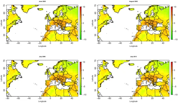
79 80 −80 −60 −40 −20 0 20 40 30 40 50 60 70 Longitude Latitude −10 −5 0 5 10 June 2003 a −80 −60 −40 −20 0 20 40 30 40 50 60 70 Longitude Latitude −10 −5 0 5 10 August 2003 b −80 −60 −40 −20 0 20 40 30 40 50 60 70 Longitude Latitude −10 −5 0 5 10 July 2006 c −80 −60 −40 −20 0 20 40 30 40 50 60 70 Longitude Latitude −10 −5 0 5 10 July 2015 d

Fig. 1: Monthly mean temperature anomalies over land areas (NCEP dataset with reference to the 1948-2015 mean) for the four case studies (in °C). The black rectangles indicate the regions of interest for the rest of the study.

We observe a significant linear temperature trend (p − value < 0.05), related to climate change, for each

81

month and region studied (red lines in figure 2): 0.23 °C per decade for June (WE), 0.24 °C for July (NE

82

and SE) and 0.25 °C for August(WE). For the rest of the study we calculate detrended temperatures

83

using a non-linear trend, calculated with a cubic smoothing spline (green lines in figure 2). The reason is

84

to extract the role of circulation in high temperature extremes, regardless of the state of the background

85

climate, the evolution of which is non-linear.

86 87 1950 1960 1970 1980 1990 2000 2010 −2 −1 0 1 2 3 4 year temper ature June (WE) a 1950 1960 1970 1980 1990 2000 2010 −2 −1 0 1 2 3 4 year temper ature August (WE) b 1950 1960 1970 1980 1990 2000 2010 −2 −1 0 1 2 3 year temper ature July (NE) c 1950 1960 1970 1980 1990 2000 2010 −2 −1 0 1 2 3 year temper ature July (SE) d

Fig. 2: Evolution of the monthly temperature anomalies averaged over the regions defined in figure 1. The red line corresponds to the linear trend, which is significant (p − value < 0.05) in all cases. The green line corresponds to a non linear trend calculated with a cubic smoothing spline.

2.2 Flow analogues

88

We used flow analogues to extract the contribution of circulation dynamics to the chosen heatwave events

89

comparing their temperature anomalies to those of analogues. Analogues were defined as the N days with

90

the most similar detrended sea level pressure (SLP) or geopotential height at 500 hPa (Z500) anomaly

91

fields. The similarity was measured with the Euclidean distance between two maps (Yiou 2014). We only

92

considered the days within a 61 calendar days (30 days before and 30 days after) window centered on

93

the day of interest because of the seasonal cycle of both circulation and temperature (Yiou et al 2012).

We further exclude the days coming from the same year as the event from the 1948–2015 data set,

be-95

cause of the persistence of the circulation. The program used to compute analogues CASTf90 is available

96

online (https://a2c2.lsce.ipsl.fr/index.php/licences/file/castf90?id=3). Once the analogues

97

were selected, we came back to the observable of interest (the detrended temperature anomalies) on those

98

selected days. The whole process is summarized in figure 3.

99 100 Day d, Year y d,y d±30,y’≠y Extreme observable (Temperature) Corresponding circulation (Z500 detrended) N best analogues

1

2

N

N

2

1

?

Fig. 3: A day with an extreme temperature anomaly (map on the top left) has a corresponding circulation, represented by the geopotential at 500 hPa (map on the bottom left). Flow analogues are days within the database which have a similar circulation to the day of interest (maps on the bottom right). The temperature anomalies of the analogues (maps on the top right) are then compared to the temperature anomalies of the day of interest (map on the top left).

Days of the event Corresponding analogues Randomly picked analogue

01/07/2015 ana1

1,ana21,. . . ,anaN1 anai1

02/07/2015 ana1 2,ana22,. . . ,ana N 2 ana i 2 .. . ... ... 31/07/2015 ana1

31,ana231,. . . ,anaN31 anai31

Table 1: Simulation of uchronic months using randomly picked analogues for July 2015. 2.3 Reconstruction of temperature distributions

101

Our goal is to reconstruct the probability distribution of detrended temperature anomalies conditional

102

to the atmospheric circulation. For this, we consider a day i, with a temperature Ti and a circulation

103

Ciwith N analogues Ci1. . . , CiN. The circulation analogues ana1i. . .anaNi provide N copies of detrended

104

temperature anomalies. Hence, we can recreate a sequence of daily temperature anomalies over a month

105

by randomly picking one of the N best analogues for each day. The resulting monthly mean

tempera-106

ture anomaly is called uchronic, because it is a temperature anomaly that might have occurred for a

107

given circulation pattern sequence. By reiterating this process, we recreated probability distributions of

108

uchronic monthly detrended temperature anomalies conditional to the atmospheric circulation. We then

109

compared this distribution to a distribution built from random days instead of analogues. In the rest

110

of the article, we set the number of random iterations to 1000. This procedure is a simplified version of

111

the stochastic weather generator of Yiou (2014), who also used weights based on the distances of the

112

analogues. Table 1 illustrates this process for the July 2015 case.

113 114

3 Parameter sensitivity tests

115

The presented method depends on a few parameters. Their choice has an influence on both the results

116

and their robustness. The following section explores the role of those parameters and how tuning them

117

may give us further information on the relationship between circulation patterns and extreme

tempera-118

ture anomalies. We also want to know whether those parameters should depend on the specific event or

119

not. This determines how general the approach can be and therefore its potential application to future

120

events and other extra-tropical regions. In particular, we studied the role played by physical parameters:

121

the variable on which the analogues are computed (SLP or Z500), the choice of the size of the domain

122

on which the analogues are computed, and the length of the dataset, and a statistical parameter: the

123

number N of analogues we kept.

124 125

3.1 Variable representing the circulation

126

SLP (e.g. Cassou and Cattiaux 2016; Sutton and Hodson 2005; Della-Marta et al 2007) and Z500 (e.g.

127

Horton et al 2015; Quesada et al 2012; Dole et al 2011) are the most commonly used variables to study

128

the atmospheric circulation. We calculated analogues using either the detrended SLP or the detrended

129

Z500. The detrending was needed due to the dependence of Z500 on lower tropospheric temperatures,

130

which are increasing due to anthropogenic climate change. We also detrended SLP since we found a small

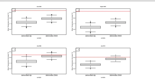
detrended slp detrended Z500 0 1 2 3 June 2003 variable Mean T emper ature Anomaly[°C] a detrended slp detrended Z500 0 1 2 3 August 2003 variable Mean T emper ature Anomaly[°C] b detrended slp detrended Z500 0 1 2 3 July 2006 variable Mean T emper ature Anomaly[°C] c detrended slp detrended Z500 0 1 2 3 July 2015 variable Mean T emper ature Anomaly[°C] d

Fig. 4: The probability density of uchronic temperature anomalies from circulation analogues generated using detrended SLP (left boxplot of each subfigure) or detrended geopotential height at 500 hPa (right boxplot of each subfigure) for each case study: June 2003 (a), August 2003 (b), July 2007 (c), July 2015 (d). The red line represents the observed detrended temperature anomaly of the event. The three lines composing the boxplot are respectively from bottom to top, the 25th (q25), median (q50) and 75th quantiles (q75). The value of the upper whiskers is min(1.5 × (q75 − q25) + q50, max(temperature anomaly)). The value of the lower whiskers is its conjugate.

significant positive trend of mean monthly SLP over the North Atlantic domain for the 1948-2015 period.

132 133

The detrending of SLP and Z500 was done by computing a monthly spatial average of those fields.

134

Then a non-linear trend was calculated with a cubic smoothing spline (Green and Silverman 1994), in

135

order to take into account the non linearity of climate change. This trend was removed to daily fields,

136

which preserves the circulation patterns. We calculated the trends for both the North Atlantic region

137

and the smaller regions on which the analogues are calculated. The differences between the trends for

138

both regions were small. We did the detrending on the North Atlantic region in this study because the

139

uncertainties on circulation patterns are amplified for smaller regions, especially as the NCEP reanalysis

140

I grid is coarse (with a resolution of about 210km).

141 142

The uchronic detrended temperature anomalies for each event that were calculated using analogues

143

of detrended SLP or detrended Z500 are shown in figure 4. The analogues computed using Z500 give

144

uchronic temperature anomalies closer to the observed detrended temperature anomaly of the event than

145

those computed using SLP. For the July 2015 case with an observed detrended temperature anomaly of

146

2.06 °C for example the mean of uchronic temperature anomalies calculated using SLP is 0.73 °C while

147

the mean uchronic temperature anomaly calculated using Z500 is 1.76 °C. The results are qualitatively

148

similar for the other cases. The better performance of the Z500 analogues compared to the SLP analogues

149

is probably related to the heat low process (e.g. Portela and Castro 1996). Warm anomalies of surface

150

temperature lead to convection. The elevation of warm air masses creates a local depression, which adds

on top of an anticyclonic anomaly a cyclonic anomaly. This flattens the SLP patterns and blurs the

152

signal, which does not happen with Z500. By using Z500 we also avoid any influence of the relief. Hence,

153

we kept the detrended Z500 to compute the analogues for the rest of the study.

154 155

3.2 Size of the domain

156

The scale on which we compare circulation patterns plays a key role in the computation of the analogues.

157

If the domain is too large, the system becomes too complicated, with too many degrees of freedom. The

158

analogues could consequently only extract a low frequency signal, like the seasonal cycle. Van den Dool

159

(1994) evaluates that it would take 1030 _{years of data to find two matching observed flows for analogues}

160

computed over the Northern Hemisphere. If we choose too small a domain, then we cannot study the role

161

of the synoptic circulation. So, on the one hand, it is no use to calculate analogues on whole hemispheres,

162

and on the other hand, we do not want to select domains which are smaller than the typical scale of

163

extra-tropical cyclones (1000 km approximately). Radanovics et al (2013) investigated automatic

algo-164

rithms to adjust the domain size of the analogues for precipitation. Here, we prefer to select a domain

165

that yields an a priori physical relevance to account for the most important features of the flow that

166

affects high temperatures in Europe.

167 168

The ideal size of the domain reveals the scale at which the processes are relevant and may very well vary

169

from one event to the other. This especially applies for studies on other types of events such as heavy

170

precipitation, droughts or storms. We compared three different domains shown in figure 5 (right hand

171

side):

172

– a large domain (the whole maps in figure 5), including the North Atlantic region, which corresponds

173

to the domain usually used to calculate weather regimes (Vautard 1990; Michelangeli et al 1995),

174

– a medium domain (the golden rectangles in figure 5), centered on Europe, which is much smaller than

175

the North Atlantic domain while being common to all events, and

176

– a small domain tailored for each event (the purple rectangles in figure 5), depending on the circulation

177

pattern of the specific summer .

178

The results are displayed on the left hand side of figure 5. The detrended temperature anomalies of

179

the heatwaves of interest, shown by the red lines, are better reproduced using the smaller domains to

180

calculate the circulation analogues for all four cases. This is because there are circulation patterns

in-181

cluded in the North Atlantic domain which probably play no role in the establishment of a heatwave

182

over Europe. For example in July 2015 we observe an important anticyclonic anomaly over Greenland. It

183

adds a constraint on the analogues while supposedly playing no role on the lesser anticyclonic anomaly

184

over the Northern Mediterranean region. The standard deviation of the uchronic detrended temperature

185

anomalies also decreases with the size of the domain.

186 187

It is relevant to rely on standard domains for a first estimation of the role played by the circulation in

188

the occurrence of a heatwave, for example by using the regions defined in Field and Intergovernmental

189

Panel on Climate Change (2012). However, for a finer analysis focused on one specific heatwave, or a

190

few given events, the choice of a tailored small domain gives better results. In the rest of the study, we

191

hence kept the smaller domains.

192 193

large medium small 0 1 2 3 June 2003 domain size Mean T emper ature Anomaly[°C] a −80 −60 −40 −20 0 20 40 30 40 50 60 70 Longitude Latitude −200 −100 0 100 200 June 2003 e

large medium small

0 1 2 3 August 2003 domain size Mean T emper ature Anomaly[°C] b −80 −60 −40 −20 0 20 40 30 40 50 60 70 Longitude Latitude −200 −100 0 100 200 August 2003 f

large medium small

0 1 2 3 July 2006 domain size Mean T emper ature Anomaly[°C] c −80 −60 −40 −20 0 20 40 30 40 50 60 70 Longitude Latitude −200 −100 0 100 200 July 2006 g

large medium small

0 1 2 3 July 2015 domain size Mean T emper ature Anomaly[°C] d −80 −60 −40 −20 0 20 40 30 40 50 60 70 Longitude Latitude −200 −100 0 100 200 July 2015 h

Fig. 5: Dependence of the probability density of uchronic detrended temperatures on the size of the domain. The maps on the right column represent the detrended Z500 monthly anomaly (m). The purple rectangles indicate the smallest zones of computation of flow analogues. The golden rectangles indicate the medium zone of computation of flow analogues. The large zone is the whole map. The boxplots of the left column display the distribution of the 1000 uchronic monthly detrented temperature constituted from randomly picked analogues. The color of the boxplot corresponds to the color of the rectangle delineating the region on which the analogues are computed. The red lines on the left hand side of the figure represent the observed detrended temperature of the case studies, from top to bottom : June 2003, August 2003, July 2006, July 2015.

3.3 Length of the dataset

194

The NCEP dataset contains 68 years. Although the recombination of analogues allows to recreate new

195

events, the dataset is finite and hence does not cover the whole range of possible events. For example, if

196

the circulation leading to a heatwave has a return period of more than the dataset length, there might

197

not be similar circulation patterns in the dataset. In this situation, the computed analogues will not be

198

a good proxy of the circulation of interest. Furthermore, even if there are close daily analogues to the

199

daily circulation of the event, it might not account for other thermodynamical processes that may or

200

may not happen simultaneously and lead to extreme temperatures. This shortcoming is called sampling

201

uncertainty (Committee on Extreme Weather Events and Climate Change Attribution 2016, Chap. 3),

202

related to the fact that the past is one occurrence of many realizations which could have happened for

203

a given state of the climate.

204 205

In order to get an order of magnitude of that uncertainty in the reconstruction of probability densities

206

of temperature anomalies we used a 500 years long pre-industrial run from CMIP5 (Taylor et al 2012).

207

The model used is GFDL-ESM2M (Dunne et al 2012, 2013). We chose this model because it was the

208

model available on the IPSL data center with the longest run for both the temperature and the Z500.

209

We selected one heatwave similar to July 2015, both in terms of temperature anomaly (compared to the

210

detrended anomaly of July 2015) and circulation patterns (see figure 6). We assume that the internal

211

variability of the model is similar to the internal variability of the reanalysis.

212 213 −80 −60 −40 −20 0 20 40 30 40 50 60 70 Longitude Latitude −10 −5 0 5 10

Monthly mean temperature anomaly

a −80 −60 −40 −20 0 20 40 30 40 50 60 70 Longitude Latitude −200 −100 0 100 200

Monthly mean anomaly of Z500

b

Fig. 6: Temperature anomaly (a) and Z500 anomaly (m) (b) of a July month from GFDL-ESM2M CMIP5 pre-industrial control run similar to July 2015.

Analogues were computed for 60 different subsets of the 500 year dataset. The lengths of the subsets

214

were 33, 68, 100 and 200 years (e.g. subsets of 68 consecutive years each, starting every 5 years of the

215

data set). We then compared the means of the uchronic temperature anomaly distributions for the

cho-216

sen July 2015-like month to one another for different subset lengths. The spread of the mean uchronic

217

temperature anomalies calculated this way gives an estimation of the uncertainty related to the limited

218

length of the dataset.

219 220

Figure 7 displays the results for subsets of 33, 68, 100 and 200 years. When the number of years of the

221

subset decreases, the spread of the mean uchronic temperature anomalies increases, going up to

approx-222

imately 0.71 °C for the 33 years subsets, 0.62 °C for 68 years, 0.36 °C for 100 years, and 0.14 °C for 200

223

years. This information is precious to determine in which measure smaller datasets are relevant for this

224

methodology. It means for example that differences of up to 0.71 °C in the mean uchronic temperatures

225

calculated from 33 years long subsets can possibly occur due to internal variability without strictly

need-226

ing additional forcing.

227 228 33 68 100 200 0.0 0.5 1.0 1.5 2.0 2.5

length of the dataset [years]

Mean T

emper

ature Anomaly[°C]

Fig. 7: Sensitivity to interdecadal variability depending on the length of the dataset. Distributions of the mean uchronic temperature anomalies for 60 different subsets of varying sizes (33, 68, 100, or 200 years) from a 500 years long pre-industrial control run (model GFDL-ESM2M) for the small domain of analogues computation.

The ability to find analogues close to the circulation of interest is related to both the size of the dataset

229

and the size of the domain on which the analogues are computed (Van den Dool 1994). It means that the

230

analogues method will get more and more accurate as the reanalysis dataset extends in the years to come.

231 232

3.4 Number of analogues

233

For the reconstruction of events by recombination of analogues, we kept the N best analogues. The

234

choice of N has an influence on both the uchronic detrended temperature anomalies and the statistical

robustness of the study. The best uchronic detrended temperature anomalies are closer to the observed

236

detrended temperature anomalies of the actual events for all case studies

237

4 The role of circulation in heatwaves

238

With the parameters kept (Z500, small domains, 68 years reanalysis data, and 20 analogues) we simulated

239

1000 uchronic detrended monthly mean temperature anomalies for each of the four selected heatwave

240

events (see the analogues boxplots in figure 8). The circulation contribution corresponds to the mean

241

of the uchronic temperature anomaly distribution simulated using circulation analogues. The spread of

242

the boxplots is due to the range of other processes which can, for a given circulation, lead to different

243

temperature anomalies.

244

In order to measure the contribution of the circulation we compared the distribution of uchronic

de-245

trended temperature anomalies with a control distribution built using random days (Control-1 boxplots

246

on figure 8). The control distribution is supposed to represent monthly detrended temperature anomalies

247

for the given month and the given region without focusing on specific circulation patterns. However, the

248

variability of random summers built that way is not realistic because the dependence between

consecu-249

tive days is not accounted for. Analogues are by construction dependent from one another, because they

250

are calculated using maps from consecutive (hence correlated) days, whereas randomly picked days are

251

independent.

252 253

In order to create a more realistic distribution of temperature anomalies using random days, we also

254

calculated detrended monthly mean temperature anomalies by using only one out of M days. M is a

255

measure of the persistence of the circulation that is accounted for. We computed the autocorrelation of

256

the detrended Z500 NCEP dataset for summer months (JJA) on each of the four small domains, for each

257

grid point, with lags from 1 to 20 days (similar to Yiou et al (2014)). For more than 10 days, the

auto-258

correlations median tends to an asymptotic value of approximately 0.1. For three days, the median of the

259

autocorrelation distribution is of approximately 0.65. For four days, it decreases to 0.45. Since the regions

260

are small, the number of degrees of freedom is small too, which means that an autocorrelation of 0.45

261

is negligible. We hence arbitrarily decided to set M=3 (Control-3 boxplots on figure 8). The circulation

262

during heatwaves corresponds to a long-lasting blocking situation, hence the persistence is probably more

263

than three days. This underestimation, combined with the limited length of the dataset explains why the

264

studied events are all outside of the distributions calculated using random days subsampled every 3 days.

265 266

For every event, the circulation plays a significant role in the occurrence of the extreme. It only explains a

267

part of it, more or less significant depending on the event. Indeed, it explains 38% of the anomaly for

Au-268

gust 2003, 57% for June 2003, 81% for July 2015 and 92% for July 2006. Considering only the uchronic

269

detrended temperature anomaly distribution, the observed heatwave is plausible given the large-scale

270

trends and the circulation for both July 2006 and July 2015. Indeed the observed detrended

tempera-271

ture anomaly is within 2 σ of the uchronic detrended temperature anomaly distribution. The circulation

272

together with the subtracted large-scale trend could explain the observed temperature anomaly. This is

273

not the case for June and August 2003 where the observed detrended temperature anomaly is

respec-274

tively 6.1 σ and 8.6 σ above the mean of the uchronic detrended temperature distribution (see table

275

2). The smaller standard deviation of the uchronic detrended temperature distribution compared to the

276

random ones shows the effect of the analogues, that is to select a part of the distribution conditioned to

277

the flow. Indeed the standard deviation of the uchronic detrended temperature anomaly distribution is

Event Observed detrended

temperature anomaly Mean detrended uchronictemperature anomaly Difference expressed as number of σ of theuchronic distribution

06/2003 3.3 °C 1.9 °C 6.1

08/2003 3.2 °C 1.2 °C 8.6

07/2006 2.5 °C 2.3 °C 0.9

07/2015 2.1 °C 1.7 °C 1.6

Table 2: Observed detrended temperature anomaly compared to the mean detrended uchronic tempera-ture anomaly for each case study.

approximately a third of the standard deviation of the temperature anomaly distribution using random

279

days taking into account the persistence of the circulation (Control-3 ). Both standard deviations might

280

be slightly underestimated due to persistence that was not accounted for. In the case of the uchronic

281

temperature anomalies this can happen due to the random pick among the analogue days and for the

282

Control-3 due to situations with more than 3 days of persistence that are not accounted for.

283 284

Control−1 Control−3 Analogues

−2 −1 0 1 2 3 June 2003 Mean T emper ature Anomaly [°C] a

Control−1 Control−3 Analogues

−2 −1 0 1 2 3 August 2003 Mean T emper ature Anomaly [°C] b

Control−1 Control−3 Analogues

−2 −1 0 1 2 3 July 2006 Mean T emper ature Anomaly [°C] c

Control−1 Control−3 Analogues

−2 −1 0 1 2 3 July 2015 Mean T emper ature Anomaly [°C] d

Fig. 8: Probability distributions of uchronic detrended monthly temperature anomalies simulated using random days (left boxplot of each subfigure), random days subsampled every three days to correct for serial dependence (middle boxplot of each subfigure) and analogues (right boxplot of each subfigure) for each case study: June 2003 (a), August 2003 (b), July 2007 (c), July 2015 (d). The red line represents the observed detrended temperature anomaly of the event.

In order to contextualize the four case studies, we reproduced the same kind of probability density

func-285

tion experiments for the same regions from 1948 to 2015 (figure 9). We calculated the uchronic detrended

286

temperature anomaly distributions for the months of June from 1948 to 2015 on the regions (both the

287

temperature and the circulation regions) defined for June 2003 (figure 9 a)). We did the same for the

288

other three events. This type of recontextualisation can be interpreted as an estimation of how extreme

289

an event really is, with respect to its atmospheric circulation.

290 291

The observed monthly mean detrended temperature anomaly falls between the 10th and 90th percentiles

292

of the uchronic detrended temperature anomaly distribution for more than half of the years between 1948

293

and 2015. It falls between the 1st and 99th percentiles for more than two thirds of the years, even though

294

the uchronic temperature anomaly distribution has a small spread compared to the total distribution.

295

The years with observed detrended temperature anomalies out of interval between the 1st and 99th

per-296

centile correspond mostly to large detrended temperature anomalies with absolute value > 0.5 °C. For

297

less than a quarter of the years between 1948 and 2015 the mean of the uchronic detrended temperature

298

anomaly distribution has a sign different from the observed detrended temperature anomaly. Those years

299

correspond to low detrended temperature anomalies with absolute values < 0.5 °C.

300 301

5 Discussion

302

The median of the uchronic temperature anomaly distribution is generally different from the observed

303

temperature anomaly. In some cases, the observed detrended temperature anomaly (red line on figure 8)

304

is not even in the uchronic temperature anomaly distribution. On figure 8 for June and August 2003, and

305

for some of the years on figure 9, this is the case (indeed, the monthly detrended temperature anomalies

306

for both months are higher than 3 °C). This difference shows caveats in the methodology, and that some

307

heatwave events cannot be explained only by their circulation.

308 309

Flow analogues are unable to reproduce the role played by the soil-moisture feedback. Indeed, the

ana-310

logues do not take into account the history of the heatwave. Extreme heatwaves happen when the

311

circulation causing the initial anomaly of temperature lasts more than a few days. As soil moisture

be-312

comes limited, the cooling of the atmosphere through evapotranspiration gets weaker, which exercises a

313

positive feedback on the temperature. Seneviratne et al (2010) isolates a dry and a wet regime, with a

314

transition phase between both. The three temperature regions used here are prone to different

evapo-315

rative regimes. In particular, the Northern Europe region is wetter than the other two. The role of soil

316

moisture is thus less important (Seneviratne et al 2006). On the other hand, several articles (St´efanon

317

et al 2012; Fischer et al 2007) showed the role of soil moisture in the exceptional temperature anomalies

318

of summer 2003, especially for August. The analogues are picked without any condition on the previous

319

days or soil moisture, and consequently they fail to reach the observed anomaly.

320 321

The main caveat of this methodology is the limited size of the dataset, which introduces an important

322

sampling uncertainty, as seen in section 3.3, and also affects the quality of the analogues. As a result,

323

the analogues might not be good enough to accurately reproduce the dynamical contribution. Indeed,

324

an extreme temperature can be related to a rare circulation, the like of which might not be found in

325

a short dataset. The distances between the analogues and the event, as well as their correlations, are

326

indices to evaluate the relevance of the analogues in each case. A better definition of what is a good

analogue will require further studies. Depending on the magnitude of the studied event, it might not

328

be possible to reconstruct a comparable month by resampling the days in the dataset. This is the case

329

for both June and August 2003, which have temperature anomalies about one degree Celsius above all

330

the other years, despite the detrending. If the event is too rare, it will not be possible to reconstitute

331

uchronic temperature anomalies close to the observed ones.

332 333

Another limitation relates to the coherence of the uchronic summers computed using analogues. Due to

334

the persistence of the circulation, the analogues we picked for each day are correlated to one another.

335

Indeed, analogues of following -and thus correlated- days are not independent. In our case, we picked

336

the 20 best analogues for each day. For each event we hence have an ensemble of 20 times the number

337

of days of the month analogues. A proof of the correlation between analogues of following days is that

338

only half of the analogues in this ensemble are unique. However, the persistence is still underestimated

339

compared to real summers. Consequently, the spread of the computed uchronic temperature anomaly

340

distributions is underestimated.

341 342

Lastly, this article only considers one month-long heatwaves, while some events as short as three

consecu-343

tive days can be considered as heatwaves (Russo et al 2015). We have tested how the length of heatwaves

344

affect the uncertainties of the method using a test similar to the one used in section 3.3, for events of

345

different length (not shown here). The sampling uncertainty on the mean uchronic temperature anomaly

346

decreases for longer events. It also seems that it can differ from one week-long event to the other. For

347

a week-long events, the probability to only have days with poor analogues is higher than for longer

348

events, especially if we deal with unusual events in terms of atmospheric circulation. Since the reasons

349

behind those differences relate to the quality of analogues, we intend to treat this more thoroughly in

350

further studies. However, we recommend to accompany any study using analogues as presented in this

351

article with an evaluation of the sampling uncertainty to validate the relevance of the methodology. This

352

evaluation could be based on pre-industrial runs similar to what is displayed here in section 3.3 or on

353

large ensembles of simulations.

354

6 Conclusion

355

This paper proposes to quantify the role of the atmospheric circulation in the occurrence of an extreme

356

monthly anomaly of temperature. The strength of our methodology is that it is easily adaptable to other

357

regions, and to other events. The parameter sensitivity tests of section three provide general guidelines

358

to choose flow analogues to investigate European summer heatwaves. It is best to use detrended Z500 as

359

a proxy of circulation, and to compile the analogues on a small domain centered on the Z500 anomaly

360

concomitant to the event. We also advise to use as long a dataset as possible.

361 362

The results on parameter sensitivities have potential implications for applications of the analogue method

363

in a downscaling or reconstruction context as well. The questions of the predictor variable (or variables),

364

that is the circulation proxy, is relevant in the downscaling context but may vary depending on the

365

predictand variable. The question of domain size has been treated by several authors (e.g. Chardon et al

366

2014; Radanovics et al 2013; Beck et al 2015) and the results are systematically in favor of relatively small

367

domains, in line with our findings. Tests on archive lengths larger than typical reanalysis record lengths

368

are rarely performed. The results are relevant since split-sample validation of downscaling methods is

369

common practice and our results show that splitting the limited length reanalysis record leads to large

uncertainties in the uchronic temperatures due to the limited sample size even using a relatively small

371

domain.

372 373

The reconstitution of an ensemble of uchronic temperatures for a given circulation is a first step refine

374

the approach of Cattiaux et al (2010) to extreme event attribution. Indeed, looking at changes for a given

375

circulation should reduce the signal to noise ratio of climate change versus natural variability (Trenberth

376

et al 2015) in what Shepherd (2016) calls a ”storyline approach” to extreme events attribution. There

377

are two ways to compare two worlds with and without climate change. The first one is to use climate

378

simulations with and without anthropogenic forcing. The second one is to compare observations of recent

379

years to observations from further back in time. It is then possible to detect a change between two periods

380

or two simulations outputs. One has to keep in mind that detecting a difference of temperature is not

381

enough to attribute the difference between the two to climate change, rather than to natural variability.

382

Indeed, the internal variability between the two periods could be of the same order of magnitude than

383

the difference caused by climate change. We have shown in section 3.3 that the longer the dataset, the

384

more it reduces the impact of internal variability on the results.

385 386

Since among the tested parameters only the regions of the temperature anomaly and of the geopotential

387

height field depend on the event, a diagnosis on heatwaves can be automatized and computed in less

388

than a day once the data set is available.

389 390

7 Acknowledgment

391

NCEP Reanalysis data provided by the NOAA/OAR/ESRL PSD, Boulder, Colorado, USA, from their

392

Web site at http://www.esrl.noaa.gov/psd/.

393

Program to compute analogues available online https://a2c2.lsce.ipsl.fr/index.php/licences/

394

file/castf90?id=3. PY and SR are supported by the ERC Grant A2C2 (No. 338965).

395

References

396

Beck C, Philipp A, Jacobeit J (2015) Interannual drought index variations in Central Europe related to the large-scale

397

atmospheric circulation—application and evaluation of statistical downscaling approaches based on circulation type

398

classifications. Theor Appl Climatol 121(3):713–732, DOI 10.1007/s00704-014-1267-z

399

Ben Daoud A, Sauquet E, Bontron G, Obled C, Lang M (2016) Daily quantitative precipitation forecasts based on the

400

analogue method: Improvements and application to a French large river basin. Atmos Res 169:147–159, DOI 10.1016/

401

j.atmosres.2015.09.015

402

Beniston M, Diaz HF (2004) The 2003 heat wave as an example of summers in a greenhouse climate? Observations and

403

climate model simulations for Basel, Switzerland. Glob Planet Change 44(1-4):73–81, DOI 10.1016/j.gloplacha.2004.

404

06.006

405

Cassou C, Cattiaux J (2016) Disruption of the European climate seasonal clock in a warming world. Nat Clim Change

406

(April):1–6, DOI 10.1038/nclimate2969

407

Cassou C, Terray L, Phillips AS (2005) Tropical atlantic influence on european heat waves. J Clim 18(15):2805–2811,

408

DOI 10.1175/JCLI3506.1

409

Cattiaux J, Vautard R, Cassou C, Yiou P, Masson-Delmotte V, Codron F (2010) Winter 2010 in Europe: A cold extreme

410

in a warming climate. Geophys Res Lett 37(20):1–6, DOI 10.1029/2010GL044613

411

Chardon J, Hingray B, Favre AC, Autin P, Gailhard J, Zin I, Obled C (2014) Spatial Similarity and Transferability of

412

Analog Dates for Precipitation Downscaling over France. J Clim 27(13):5056–5074, DOI 10.1175/JCLI-D-13-00464.1

Chardon J, Favre AC, Hingray B (2016) Effects of Spatial Aggregation on the Accuracy of Statistically Downscaled

414

Precipitation Predictions. J Hydrometeor 17(5):1561–1578, DOI 10.1175/JHM-D-15-0031.1

415

Ciais P, Reichstein M, Viovy N, Granier A, Ogee J, Allard V, Aubinet M, Buchmann N, Bernhofer C, Carrara A, Chevallier

416

F, De Noblet N, Friend AD, Friedlingstein P, Grunwald T, Heinesch B, Keronen P, Knohl A, Krinner G, Loustau D,

417

Manca G, Matteucci G, Miglietta F, Ourcival JM, Papale D, Pilegaard K, Rambal S, Seufert G, Soussana JF, Sanz

418

MJ, Schulze ED, Vesala T, Valentini R (2005) Europe-wide reduction in primary productivity caused by the heat and

419

drought in 2003. Nature 437(7058):529–533, DOI 10.1038/nature03972

420

Committee on Extreme Weather Events and Climate Change Attribution (2016) Attribution of Extreme Weather Events

421

in the Context of Climate Change. DOI 10.17226/21852

422

Compo GP, Whitaker JS, Sardeshmukh PD, Matsui N, Allan RJ, Yin X, Gleason BE, Vose RS, Rutledge G, Bessemoulin

423

P, Br¨onnimann S, Brunet M, Crouthamel RI, Grant AN, Groisman PY, Jones PD, Kruk M, Kruger AC, Marshall

424

GJ, Maugeri M, Mok HY, Nordli O, Ross TF, Trigo RM, Wang XL, Woodruff SD, Worley SJ (2011) The Twentieth

425

Century Reanalysis Project. Quat J Roy Met Soc 137:1–28, DOI 10.1002/qj.776.

426

Della-Marta PM, Luterbacher J, von Weissenfluh H, Xoplaki E, Brunet M, Wanner H (2007) Summer heat waves over

427

western Europe 1880-2003, their relationship to large-scale forcings and predictability. Clim Dyn 29(2-3):251–275,

428

DOI 10.1007/s00382-007-0233-1

429

Djalalova I, Delle Monache L, Wilczak J (2015) PM2.5 analog forecast and Kalman filter post-processing for the Community

430

Multiscale Air Quality (CMAQ) model. Atmos Environ 108:76–87, DOI 10.1016/j.atmosenv.2015.02.021

431

Dole R, Hoerling M, Perlwitz J, Eischeid J, Pegion P, Zhang T, Quan XW, Xu T, Murray D (2011) Was there a basis for

432

anticipating the 2010 Russian heat wave? Geophys Res Lett 38(6):1–5, DOI 10.1029/2010GL046582

433

Van den Dool H (1994) Searching for analogues, how long must we wait? Tellus A 46(3):314–324

434

Duband D (1981) Pr´evision spatiale des hauteurs de pr´ecipitations journali`eres (A spatial forecast of daily precipitation

435

heights). La Houille Blanche (7-8):497–512, DOI 10.1051/lhb/1981046

436

Dunne JP, John JG, Shevliakova S, Stouffer RJ, Krasting JP, Malyshev SL, Milly PCD, Sentman LT, Adcroft AJ, Cooke

437

W, Dunne KA, Griffies SM, Hallberg RW, Harrison MJ, Levy H, Wittenberg AT, Phillips PJ, Zadeh N (2012) GFDL’s

438

ESM2 Global Coupled Climate-Carbon Earth System Models. Part I: Physical Formulation and Baseline Simulation

439

Characteristics. J Clim 25:6646–6665, DOI 10.1175/JCLI-D-11-00560.1

440

Dunne JP, John JG, Shevliakova S, Stouffer RJ, Krasting JP, Malyshev SL, Milly PCD, Sentman LT, Adcroft AJ, Cooke

441

W, Dunne KA, Griffies SM, Hallberg RW, Harrison MJ, Levy H, Wittenberg AT, Phillips PJ, Zadeh N (2013) GFDL’s

442

ESM2 global coupled climate-carbon earth system models. Part II: Carbon system formulation and baseline simulation

443

characteristics. J Clim 26(7):2247–2267, DOI 10.1175/JCLI-D-12-00150.1

444

Feudale L, Shukla J (2007) Role of Mediterranean SST in enhancing the European heat wave of summer 2003. Geophys

445

Res Lett 34(3):L03,811, DOI 10.1029/2006GL027991

446

Field CB, Intergovernmental Panel on Climate Change (2012) Managing the risks of extreme events and disasters to

447

advance climate change adaptation: special report of the Intergovernmental Panel on Climate Change. DOI 10.1017/

448

CBO9781139177245

449

Fischer EM, Seneviratne SI, Vidale PL, L¨uthi D, Sch¨ar C (2007) Soil moisture-atmosphere interactions during the 2003

450

European summer heat wave. J Clim 20(20):5081–5099, DOI 10.1175/JCLI4288.1

451

Fouillet A, Rey G, Laurent F, Pavillon G, Bellec S, Guihenneuc-Jouyaux C, Clavel J, Jougla E, H´emon D (2006) Excess

452

mortality related to the August 2003 heat wave in France. Int Arch Occup Environ Health 80(1):16–24, DOI 10.1007/

453

s00420-006-0089-4

454

G´omez-Navarro JJ, Werner J, Wagner S, Luterbacher J, Zorita E (2014) Establishing the skill of climate field

recon-455

struction techniques for precipitation with pseudoproxy experiments. Clim Dyn 45(5-6):1395–1413, DOI 10.1007/

456

s00382-014-2388-x

457

Green PJ, Silverman BW (1994) Nonparametric regression and generalized linear models : a roughness penalty approach,

458

1st edn. Monographs on statistics and applied probability ; 58, Chapman & Hall, London ; New York, p.J. Green and

459

B.W. Silverman. ill. ; 23 cm.

460

Hamill TM, Whitaker JS (2006) Probabilistic quantitative precipitation forecasts based on reforecast analogs: Theory and

461

application. Mon Wea Rev 134(11):3209–3229, DOI 10.1175/MWR3237.1

462

Hamill TM, Scheuerer M, Bates GT (2015) Analog Probabilistic Precipitation Forecasts Using GEFS Reforecasts and

463

Climatology-Calibrated Precipitation Analyses. Mon Wea Rev 143(8):3300–3309, DOI 10.1175/MWR-D-15-0004.1

464

Horton DE, Johnson NC, Singh D, Swain DL, Rajaratnam B, Diffenbaugh NS (2015) Contribution of changes in atmospheric

465

circulation patterns to extreme temperature trends. Nature 522(7557):465–469, DOI 10.1038/nature14550

466

Kalnay E, Kanamitsu M, Kistler R, Collins W, Deaven D, Gandin L, Iredell M, Saha S, White G, Woollen J, Zhu Y, Chelliah

467

M, Ebisuzaki W, Higgins W, Janowiak J, Mo KC, Ropelewski C, Wang J, Leetmaa A, Reynolds R, Jenne R, Joseph D

468

(1996) The NCEP/NCAR 40-year reanalysis project. DOI 10.1175/1520-0477(1996)077h0437:TNYRPi2.0.CO;2, arXiv:

469

1011.1669v3

Lorenz EN (1969) Atmospheric Predictability as Revealed by Naturally Occurring Analogues. J Atmos Sci 26(4):636–646,

471

DOI 10.1175/1520-0469(1969)26h636:APARBNi2.0.CO;2

472

Michelangeli PA, Vautard R, Legras B (1995) Weather Regimes: Recurrence and Quasi Stationarity. DOI 10.1175/

473

1520-0469(1995)052h1237:WRRAQSi2.0.CO;2

474

Peng RD, Bobb JF, Tebaldi C, McDaniel L, Bell ML, Dominici F (2011) Toward a Quantitative Estimate of Future Heat

475

Wave Mortality under Global Climate Change. Environ Health Perspect (May), DOI 10.1289/ehp.1002430

476

Poli P, Hersbach H, Dee DP, Berrisford P, Simmons AJ, Vitart F, Laloyaux P, Tan DGH, Peubey C, Th´epaut JN, Tr´emolet

477

Y, H´olm EV, Bonavita M, Isaksen L, Fisher M (2016) ERA-20C: An Atmospheric Reanalysis of the Twentieth Century.

478

J Clim 29(11):4083–4097, DOI 10.1175/JCLI-D-15-0556.1

479

Portela A, Castro M (1996) Summer thermal lows in the Iberian peninsula: A three-dimensional simulation. Quat J Roy

480

Met Soc 122(1), DOI 10.1002/qj.49712252902

481

Quesada B, Vautard R, Yiou P, Hirschi M, Seneviratne SI (2012) Asymmetric European summer heat predictability from

482

wet and dry southern winters and springs. Nat Clim Change 2(10):736–741, DOI 10.1038/nclimate1536

483

Radanovics S, Vidal JP, Sauquet E, Ben Daoud A, Bontron G (2013) Optimising predictor domains for spatially coherent

484

precipitation downscaling. Hydrol Earth Sys Sc 17(10):4189–4208, DOI 10.5194/hess-17-4189-2013

485

Rebetez M, Dupont O, Giroud M (2009) An analysis of the July 2006 heatwave extent in Europe compared to the record

486

year of 2003. Theor Appl Climatol 95(1-2):1–7, DOI 10.1007/s00704-007-0370-9

487

Russo S, Sillmann J, Fischer EM (2015) Top ten European heatwaves since 1950 and their occur- rence in the future.

488

Environ Res Lett 10(12):124,003, DOI 10.1088/1748-9326/10/12/124003

489

Schenk F, Zorita E (2012) Reconstruction of high resolution atmospheric fields for Northern Europe using analog-upscaling.

490

Clim Past 8(5):1681–1703, DOI 10.5194/cp-8-1681-2012

491

Seneviratne SI, L¨uthi D, Litschi M, Sch¨ar C (2006) Land-atmosphere coupling and climate change in Europe. Nature

492

443(7108):205–209, DOI 10.1038/nature05095

493

Seneviratne SI, Corti T, Davin EL, Hirschi M, Jaeger EB, Lehner I, Orlowsky B, Teuling AJ (2010) Investigating soil

494

moisture-climate interactions in a changing climate: A review. Earth-Sci Rev 99(3-4):125–161, DOI 10.1016/j.earscirev.

495

2010.02.004

496

Shepherd TG (2015) Climate science: The dynamics of temperature extremes. Nature 522(7557):425–427, DOI 10.1038/

497

522425a

498

Shepherd TG (2016) A Common Framework for Approaches to Extreme Event Attribution. Current Climate Change

499

Report 2:28–38, DOI 10.1007/s40641-016-0033-y

500

St´efanon M, Drobinski P, D’Andrea F, De Noblet-Ducoudr´e N (2012) Effects of interactive vegetation phenology on the

501

2003 summer heat waves. J Geophys Res Atmospheres 117(24):1–15, DOI 10.1029/2012JD018187

502

Sutton RT, Hodson DLR (2005) Atlantic Ocean Forcing of North American and European Summer Climate. Science

503

309(5731):115–118, DOI 10.1126/science.1109496

504

Tandeo P, Ailliot P, Ruiz J, Hannart A, Chapron B, Easton R, Fablet R (2015) Combining analog method and ensemble

505

data assimilation: application to the Lorenz-63 chaotic system. Machine Learning and Data Mining Approaches to

506

Climate Science pp 3–12, DOI 10.1007/978-3-319-17220-0 1

507

Taylor KE, Stouffer RJ, Meehl Ga (2012) An Overview of CMIP5 and the Experiment Design. Bull Amer Met Soc

508

93(4):485–498, DOI 10.1175/BAMS-D-11-00094.1

509

Toth Z (1991) Estimation of Atmospheric Predictability by Circulation Analogs. Mon Wea Rev 119(1):65–72

510

Trenberth KE, Fasullo JT, Shepherd TG (2015) Attribution of climate extreme events. Nat Clim Change 5(August):725–

511

730, DOI 10.1038/nclimate2657

512

Turco M, Quintana Segu´ı P, Llasat MC, Herrera S, Guti´errez JM (2011) Testing MOS precipitation downscaling for

513

ENSEMBLES regional climate models over Spain. J Geophys Res 116:D18,109, DOI 10.1029/2011JD016166

514

Vanvyve E, Monache LD, Monaghan AJ, Pinto JO (2015) Wind resource estimates with an analog ensemble approach.

515

Renewable Energy 74:761–773, DOI http://dx.doi.org/10.1016/j.renene.2014.08.060

516

Vautard R (1990) Multiple Weather Regimes over the North Atlantic: Analysis of Precursors and Successors. Mon Wea

517

Rev 118, DOI 10.1175/1520-0493(1990)118h2056:MWROTNi2.0.CO;2

518

Yiou P (2014) AnaWEGE: A weather generator based on analogues of atmospheric circulation. Geosci Model Dev 7:531–

519

543, DOI 10.5194/gmd-7-531-2014

520

Yiou P, Nogaj M (2004) Extreme climatic events and weather regimes over the North Atlantic: When and where? Geophys

521

Res Lett 31:1–4, DOI 10.1029/2003GL019119

522

Yiou P, Salameh T, Drobinski P, Menut L, Vautard R, Vrac M (2012) Ensemble reconstruction of the atmospheric column

523

from surface pressure using analogues. Clim Dyn 41(5-6):1333–1344, DOI 10.1007/s00382-012-1626-3

524

Yiou P, Boichu M, Vautard R, Vrac M, Jourdain S, Garnier E, Fluteau F, Menut L (2014) Ensemble meteorological

525

reconstruction using circulation analogues of 1781-1785. Clim Past 10(2):797–809, DOI 10.5194/cp-10-797-2014

526

Zorita E, von Storch H (1999) The analog method as a simple statistical downscaling technique: Comparison with more

527

complicated methods. J Clim 12(8):2474–2489, DOI 10.1175/1520-0442(1999)012h2474:TAMAASi2.0.CO;2

−3 −2 −1 0 1 2 3 June (WE) years

Mean detrended temper

ature anomaly [°C] 1950 1955 1960 1965 1970 1975 1980 1985 1990 1995 2000 2005 2010 2015 a −3 −2 −1 0 1 2 3 August (WE) years

Mean detrended temper

ature anomaly [°C] 1950 1955 1960 1965 1970 1975 1980 1985 1990 1995 2000 2005 2010 2015 b −3 −2 −1 0 1 2 3 July (NE) years

Mean detrended temper

ature anomaly [°C] 1950 1955 1960 1965 1970 1975 1980 1985 1990 1995 2000 2005 2010 2015 c −3 −2 −1 0 1 2 3 July (SE) years

Mean detrended temper

ature anomaly [°C]

1950 1955 1960 1965 1970 1975 1980 1985 1990 1995 2000 2005 2010 2015

d

Fig. 9: Evolution of the detrended temperature distributions for all the months of June in Western Europe (a), August in Western Europe (b), July in Northern Europe (c) and July in Southern Europe (d). The regions are displayed in figure 1. The red dots correspond to the observed detrended temperature anomaly for each year.