HAL Id: hal-01722062
https://hal.archives-ouvertes.fr/hal-01722062
Submitted on 2 Mar 2018HAL is a multi-disciplinary open access
archive for the deposit and dissemination of sci-entific research documents, whether they are pub-lished or not. The documents may come from teaching and research institutions in France or abroad, or from public or private research centers.
L’archive ouverte pluridisciplinaire HAL, est destinée au dépôt et à la diffusion de documents scientifiques de niveau recherche, publiés ou non, émanant des établissements d’enseignement et de recherche français ou étrangers, des laboratoires publics ou privés.
Public Domain
Abaques numériques: visualisation et post-traitement de
solutions à variable séparée. Application au temps réel
non linéaire
Felipe Bordeu, Francisco Chinesta, Elias Cueto, Adrien Leygue
To cite this version:
Felipe Bordeu, Francisco Chinesta, Elias Cueto, Adrien Leygue. Abaques numériques: visualisation et post-traitement de solutions à variable séparée. Application au temps réel non linéaire. 11e colloque national en calcul des structures, CSMA, May 2013, Giens, France. �hal-01722062�
CSMA 2013
11e Colloque National en Calcul des Structures 13-17 Mai 2013
Abaques Numériques: Visualisation et Post-Traitement de Solutions à
Variable Séparée. Application au Temps Réel Non Linéaire
Felipe BORDEU1, Francisco CHINESTA1, Elias CUETO2, Adrien. LEYGUE1
1GeM, Institut de recherche en Génie civil et Mécanique UMR CNRS -ECN,[email protected] 2Aragon Institute of Engineering Research (I3A), Universidad de Zaragoza,[email protected]
Résumé — Today many solution strategies use internally some separation of variables to represent all the quantities (fields, linear operators. . .). This type of representation, in many cases, enables us to reduce drastically the amount of data to manipulate and store. But, the exploration and the post-treatment of this type of solutions is not an easy task. Mainly, because all the available software are not capable of taking into account the "separated" structure of the solutions. In this paper, we present a series of tools for the efficient storage and post-treatment of solutions in separated representation. Three application are presented : 1) the post-processing of a multidimensional solution of a mechanical problem, and the generation of the Pareto front of an associated optimisation problem, 2) the simulation in “real time” of a non linear deformable body, and an associated control problem. 3) practical application to the on-site help in the decision making process using lightweight device.
1
Introduction
The PGD (Proper General Decomposition) method [1] applied to multidimensional problems uses some kind of separation of variable to represent all the quantities of the problem to solve. In most cases, the quantities are represented as a finite sum of product of functions. For example, one possible separation is : u(x1, · · · , xdim) = modes
∑
m=1 f1m(x1) × · · · × fdimm (xdim) (1)This decomposition of the field u, called canonical decomposition, is not unique. Others decomposi-tions are possibles, like Tucker or H-Tucker [2] can be used. In this paper we focus our work on canonical decompositions only.
1.1 Multidimensional problems and PGD
The PGD method can be seen as a separation of variables strategy for finding a separated represen-tation of an unknown field, knowing only the operator of the differential equation and the right hand side term. The solution of a problem using the PGD method is done in two steps. First, we decompose all the quantities (geometry, fields, operators. . .) of the problem in a separated form (similar to equation 1). Then, the strategy in its simplest form consists in the sequential calculation of the different terms of the sum (called "mode"). This stage in the strategy is called the enrichment step. The calculation of one mode is a non linear problem addressed by a classic fixed point algorithm. The main advantage of this approach is that inside the fixed point iteration only low dimensionality problems must be solved (dimension of the coordinate space xi). This enables us to solve multidimensional problems at very low
cost.
The PGD method is capable of solving multidimensional problems in a very efficient way. This enables us to consider very challenging simulations. For example including parameters (like material properties, boundary conditions, geometrical parameters) as extra coordinates in the original problem. By post-processing these multidimensional solutions we are able to generate virtual charts or computational vademecum, that can be used to solve associated engineering design problems [3].
Some examples are :
1. finding the optimal parameters for a process, 2. identification of material properties,
3. real time simulation-based control,
4. on-site help in the decision making process using lightweight devices.
All these examples can benefit from the previously constructed computational vademecum in differ-ent ways. A very important point is that the sensitivity of the solution with respect to a coordinate can be calculated directly, e.g. :
∂u(x1, · · · , xdim) ∂xdim = modes
∑
m=1 f1m(x1) × · · · × ∂ fdimm (xdim) ∂xdim (2)1.2 Exploration of a "Virtual Chart"
The multidimensional solutions generated by the PGD method are very rich. But they must be kept in separated representation if we want to have a minimal memory footprint during exploration, because the full reconstruction of the solution is plagued by the curse of dimensionality.
With the aim of storing these solution a new file format, called PXDMF, was developed. It is based on the popular XDMF format (eXtensible Data Model and Format)1, from which it inherits all the advantages like the compressed binary storage.
The 3D visualization of a separated variable solution needs the reconstruction of the multidimen-sional solution in a smaller dimension space. This is done by fixing some dimensions in order to always reconstruct solutions in lower dimension spaces. To make this task easier a plug-in was developed for the open source software ParaView [4] This module is able to reconstruct the solution on the fly, and to calculate automatically the sensitivity of the fields with respect to the fixed coordinates.
2
The PXDMF File Format
In general, the PGD method makes use of some kind of discretization of the spaces xj (finite
ele-ments, finite difference. . .). So storing a solution in separated representation means that we have to store the spaces discretizations and all the functions fmj (xj). This means that we have to store dim space
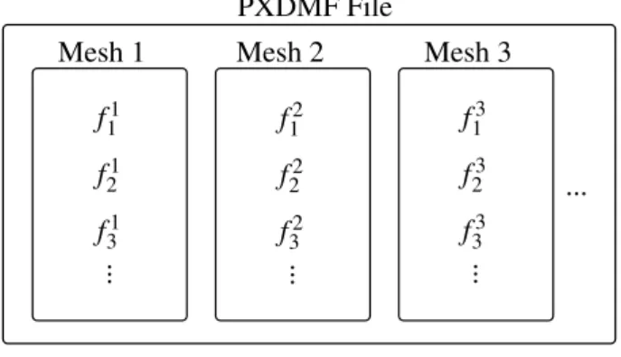
dis-cretizations, and modes fields in each discretized space (meshes and nodal values, in the case of FEM). The main idea was to use an already existing format, the requirements were ; portability, robustness, and simplicity and of course the ability to store more than one mesh. The popular XDMF format (eX-tensible Data Model and Format), fulfils all the requirements. In addition the XDMF format can handle binary and compressed data.
PXDMF File Mesh 1 ... f11 f21 f31 ... Mesh 2 f12 f22 f32 ... Mesh 3 f13 f23 f33 ...
Fig. 1 – PXDMF internal Structure
A key advantage is that the files are written using the XML language (Extensible Markup Language)2 to describe the data, making it human readable. In the case of large data, compressed binary files can be
1. www.xdmf.org
used for a more efficient storage. The complete description of the PXDMF file format can be found in our site[5].
3
The ParaView PXDMF Tools Plugin
As said before, the evaluation of the solution at a point needs the evaluation of the functions fmj . To facilitate the reconstruction and the exploration, a series of tools was developed. These tools were in the form of a plugin for the visualization software ParaView.
The name of the plugin is PXDMFReader and the current version is 1.5.2. The plugin contains a reader, capable of reading PXDMF files and a series of filters and python routines. After loading the plugin in ParaView, a new file format is available in the open menu, and a new menu bar is available.
The plug-in (in binary format) is available on the site. Videos for the installation and examples are available on the web site[5].
3.1 The PXDMF Reader
The PXDMF Reader adds support to ParaView for reading separated representation data-sets stored in PXDMF file format. The PXDMF Reader was developed to reconstruct solutions stored in separated representation in a very user-friendly way. Once the solution is reconstructed, the data can be treated with all the techniques available in ParaView.
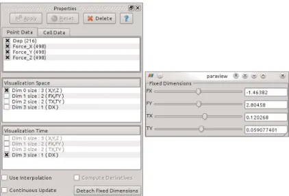
The properties of the reader are (Figure 3) :
Point Data and Cell Data : The Point (Cell) field to be loaded. If the number of Point (Cell) data modes are less than 100, then individual modes can be selected. This is used mainly for debugging pur-poses.
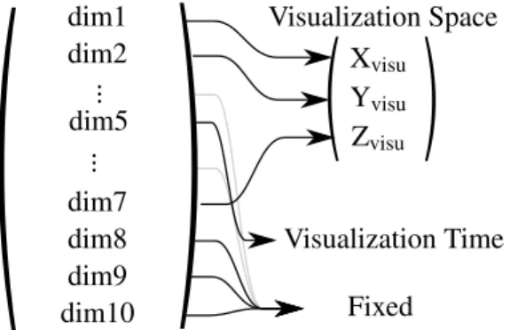
Visualization Space : The user can select the dimension(s) to put in the Visualization Space. Note : the Visualization Space can be different from the physical space of the problem. For example, an arbitrary parametric dimension can be selected and mapped to any dimension of the Vizualisation Space (Figure 2).
Visualization Time : The user can select a one-dimensional dimension to put in the Visualization Time. Again the Visualization Time can be different from the temporal dimension of the problem. Any unidimensional dimension can be in the Visualization Time (Figure 2).
dim1 ... ... Fixed dim2 dim5 dim8 dim10 Xvisu Yvisu Zvisu Visualization Time dim9 dim7 Visualization Space
Fig. 2 – Mapping from the problem space to the Visualizaton Space and Time
Use Interpolation : This activate the use of the interpolation generated by the mesh. So the field can be computed at any point in the space. For example, between two point in a temporal dimension. If this check-box is not checked the closest point is used for the reconstruction.
Compute Derivatives : Compute Derivatives requires "Use Interpolation" to be enabled. When this option is enabled, the sensibility of the Point fields are automatically calculated with respect to the Fixed Dimensions and to the Temporal Dimension.
Continuous Update : This option enables us to bypass the need of clicking on the Apply button every time that we change a Fixed dimension. So the solution is updated in real-time (be careful not to use this option with very big data-sets).
Detach Fixed Dimensions : This button enables us to detach the Fixed Dimensions sliders so they can be changed easily.
Fixed Dimensions : All the dimension not in the Visualization Space neither in the Visualization Time. Figure 3, shows the same dialog in a "Detach Fixed Dimension" mode with the first dimension ("Dim 0 size : 3 (X,Y,Z)") in the Visualization Space, and the fourth dimension ("Dim 3 size : 1 (DX)") in the Visualization Time. The two mapped spaces are automatically removed from the "Fixed Dimension" dialog.
The information about the names (and the units ) of the dimensions used in the Visualization Space is passed to the generated solution, so if the user activates the option "Show cube axes" correct labels are generated.
Fig. 3 – Properties Dialog with X,Y,Z in the Visualization Space, DX in the Visualization Time and with Detached Fixed Dimensions
4
The Filters
Four filters are available in the plugin. The aim of these filter is to make easier some operations related with the separated representation of the solutions.
A new toolbar and a new sub-menu (Figure 4) inside the filter menu are available.
Fig. 4 – (Left) The PXDMF toolbar, (Right) The PXDMF menu on the Filter menu of ParaView
4.1 Annotate Fixed Dimension Data Filter
This filter enable one to annotate all the Fixed Dimension data including the Visualization Time dimension.The format of the annotation can be changed in the properties of the filter using C style format.The %f correspond to the format of the value and the %s correspond to the format of the unit (if present).
4.2 Calculator With Global Data Filter
The "Calculator With Global Data" filter computes a new data array or new point coordinates as a function of existing scalar or vector arrays. This filter is based on the original Calculator Filter available in ParaView. But adds the possibility of using global data (Fixed Dimension and Visualization Time) in the formula.
4.3 Global Data To Point Filter
The "Global Data To Point" filter creates a new point from the Global Data (Fixed dimension and Visualization Time). This filter is very useful for solution with parametric dimensions based on the physical space (e.g. position of a force, position of a crack).
4.4 Transform With Axis Filter
The "Transform With Axis" filter allows us to specify the position, size and orientation of a data sets. This filter is based on the original Transform Filter available in ParaView. Additionally this filter will move/scale/rotate the axis information. So when "Show cube axes" is enabled the axis are correctly named and correctly moved/scaled/rotated.
The "On Axes Also" option apples the transform filter on the axis of the data-set also.
This filter is very useful in the case of data with very different scales. For example, in the case of parametric data with very different units (Young modulus in one axis, and Poisson ratio in the other axis). The Young modulus normally is in the order of 10 GPa, and the Poisson ration is in the order of 1. 4.5 Python Routines
ParaView has a python console. This console allows the user to control most of the visualization using command lines. To make the control of the PXDMF Reader easier, some extra function are present in the plugin.
The class ReaderSync enables the user to synchronize and control several PXDMFReader at the same time. Additionally, extra functions are present to ease the manipulation of the camera.
note : Render() must be called to redraw the scene
5
Applications
5.1 Post-treatment and Pareto front
A first example is the post-treatment of a multidimensional solution of a mechanical problem, and the generation of the Pareto front of an associated optimisation problem. We consider a parametric model related to the elasticity problem in which parameters describing the material and the geometry are con-sidered as extra-coordinates. A basic simple (but three-dimensional) problem was treated. In addition to the three-dimensional physical space, we add three new coordinates, one related to the Young’s modulus E, one to the Poisson’s ratioν and one to the geometrical parameter e depicted in Figure 5. The bound-ary conditions are the followings : distributed surface force on the light-grey surface (red arrows), and displacement equal to zero on the dark-grey surface (left part of the left hole).
The simulation was done using the PGD method, to obtain a multidimensional solution containing the solution for any combination of material and geometrical parameters. More details about the PGD method applied to this example can be found in [3].
This problem was solved for E∈ [100,250000]MPa, ν ∈ [0,0.45] and e ∈ [1,5], using the following
decomposition. u(x, y, z, E,ν,e) = 25
∑
i=1 fxyi (x, y)· fi z(z)· f i E(E)· f i ν(ν) · fei(e) (3)Fig. 5 – Physical space parametrized by the parameter e
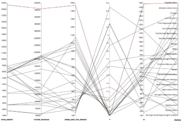
The main motivation behind this kind of problem, is to optimize the parameter e as a function of the material properties. For example, for a series of given material families we can find the optimal thickness of the piece to ensure an elastic behaviour and the weight for the given thickness.
Figure 6 shows the optimal value of e for every material in the library. One important point is that the lightest piece does not correspond to the lowest value of e.
Fig. 6 – Parameters, optimal value of e and weight for ever material in the data base
The algorithm used for the optimisation was written in python using the tools presented in the previ-ous sections.
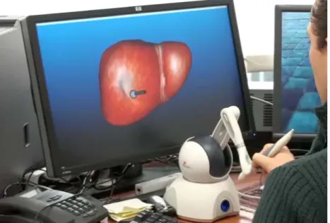
5.2 Real time simulation of a deformable body
Real time simulation is one of the most challenging scenarios for simulation-based engineering sci-ences. The term real time strongly depends on the particular application, but surgery simulation is among the most demanding ones. Haptic surgery simulators compute the response of biological soft tissues and give it back to the peripherals at, at least, 25 Hz of feedback rate if visual realism is needed, and notably 500Hz-1kHz if haptic response is desired.
on its surface. This force is parametrised by the position (px, py), the orientation (θx, θy∈ [−π/4, π/4])
and the amplitude (a ∈ [0, 1]). Additionally, we consider an extra coordinate to tune the stiffness of an embedded tumour (e ∈ [0, 5]) (e represent the rigidity factor with respect to the healthy liver tissue).
The solution was written using the following decomposition :
u(x, y, z, px, py, θx, θy, e, a) = 182
∑
i=1
Xi(x, y, z) · Pi(px, py) · Θ(θx, θy) · E(e) · A(a) (4)
Figure 7 schematically shows the haptic device and the virtual (simulated) solid.
q x
u
Haptic device Solid
Tumor
Fig. 7 – Haptic and cinematic relations
Is important to notice that the position of the force must be evaluated in the deformed configuration for realistic sensations. This means that the equation q = x + u must be satisfied for all times. Where q correspond to the position of the haptic device, x the position of the force in the reference configuration and u the displacement of point x.
This non-linear equation must be solved in real time (at 1kHz rate). As said before the sensitivity of the field (u) can be calculated directly using the equation (4). This enables us to use a Newton-Raphson algorithm for the resolution. After some tests we conclude that we need only one Newton-Raphson iteration at each haptic frame, since the algorithm is restarted 850 times per seconds with a initial guess that is very close to the solution.
Figure 8 shows a user manipulating the haptic arm at a visual frame rate of 20Hz and haptic frame rate of 850Hz.
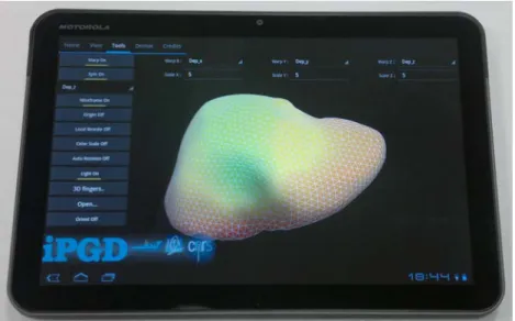
5.3 Application using a lightweight device
In most cases the computed solution can be stored in such a compact form that it is compatible with handheld devices like smartphones and tablets. For Android-operated devices, an application has been developed (iPGD, freely downloadable form [5]) that can open and post-process separated representation solutions.
The user can fix some dimensions and the application is able to reconstruct the solution and generate a visual representation (1D, 2D or 3D). These solutions can be post-processed for the calculation of associated quantities of interest.
Figure 9 shows the visualisation of a solution on a Motorola Xoom Tablet.
Fig. 9 – Visualisation of a multidimensional solution on a tablet
6
Conclusions
The PGD-based off-line/on-line approach opens numerous possibilities in the context of simulation based engineering for simulating, optimizing or controlling materials, processes and systems. The mul-tidimensional structure of these virtual charts or computational vademecum demands innovative tools to circumvent the curse of dimensionality.
Références
[1] A. Ammar, B. Mokdad, F. Chinesta, R. Keunings. A new family of solvers for some classes of multidimen-sional partial differential equations encountered in kinetic theory modeling of complex fluids, Journal of Non-Newtonian Fluid Mechanics, Vol. 139, No. 3 pp. 153-176, 2006.
[2] L. Grasedyck. Hierarchical Singular Value Decomposition of Tensors, SIAM. J. Matrix Anal. & Appl.,Vol. 31, No. 4 pp.2029-2054, 2010.
[3] F. Chinesta, A. Leygue, F. Bordeu, J.V. Aguado, E. Cueto, D. Gonzales, I. Alfaro, A. Ammar, A. Huerta. PGD-Based Computational Vademecum for Efficient Design, Optimization and Control, Archives of Computational Methods in Engineering. pp. 1-29, 2013. 10.1007/s11831-013-9080-x.
[4] A. Henderson, ParaView Guide, A Parallel Visualization Application. www.paraview.org, Kitware Inc., 2007. [5] htp://rom.research-centrale-nantes.com