HAL Id: hal-02447631
https://hal.archives-ouvertes.fr/hal-02447631v2
Preprint submitted on 22 Jan 2020
HAL is a multi-disciplinary open access
archive for the deposit and dissemination of
sci-entific research documents, whether they are
pub-lished or not. The documents may come from
teaching and research institutions in France or
abroad, or from public or private research centers.
L’archive ouverte pluridisciplinaire HAL, est
destinée au dépôt et à la diffusion de documents
scientifiques de niveau recherche, publiés ou non,
émanant des établissements d’enseignement et de
recherche français ou étrangers, des laboratoires
publics ou privés.
Machine Learning design of Volume of Fluid schemes for
compressible flows
Bruno Després, Hervé Jourdren
To cite this version:
Bruno Després, Hervé Jourdren. Machine Learning design of Volume of Fluid schemes for compressible
flows. 2020. �hal-02447631v2�
Machine Learning design of
Volume of Fluid schemes for compressible flows
Bruno Després
Sorbonne-Université, CNRS, Université de Paris, Laboratoire Jacques-Louis Lions (LJLL), F-75005 Paris, France, Institut Universitaire de France,
and Hervé Jourdren
CEA, DAM, DIF, F-91297 Arpajon, France
Université Paris-Saclay, CEA DAM DIF, Laboratoire en Informatique Haute Performance pour le Calcul et la simulation, F-91297 Arpajon , France
Abstract
Our aim is to establish the feasibility of Machine-Learning-designed Volume of Fluid algorithms for compressible flows. We detail the incremental steps of the construction of a new family of Volume of Fluid-Machine Learning (VOF-ML) schemes adapted to bi-material compressible Euler calculations on Cartesian grids. An additivity principle is formulated for the Machine Learning datasets. We explain a key feature of this approach which is how to adapt the compressible solver to the preservation of natural symmetries. The VOF-ML schemes show good accuracy for advection of a variety of interfaces, including regular interfaces (straight lines and arcs of circle), Lipschitz interfaces (corners) and non Lipschitz triple point (the Trifolium test problem). Basic comparisons with a SLIC/Downwind scheme are presented together with elementary bi-material calculations with shocks.
Keywords: VOF, CFD, ML
1. Introduction
Machine Learning (ML) [19] for the construction of numerical fluxes adapted to Finite Volume (FV) discretizations is be-coming a research subject of its own, see recent contributions for the discretization of hyperbolic equations by Hesthaven et al [30, 34]. For viscous incompressible flows, like bubble flows where the curvature of the interface controls the dynamics, it seems that ML techniques are established techniques now [37]: we refer to Zaleski et al. [28, 2] for the reconstruction of the curvature of interfaces and to [16] for an extension to compressible effects. The exact curvature is function of the second derivative of the function that defines the interface, and a comprehensive review centered on incompressible flows with surface tension is [17]. More general references can be found in [29]. On the contrary, for compressible non viscous flows, the interfaces are more related to contact discontinuities and material discontinuities: the dynamics of interfaces is more similar to the one of passive scalars; so it is needed to address interfaces with low regularity. In this context, we refer to [10, 36] for historical references on VOF methods (KRAKEN code, YOUNGS method) for compressible flows and [31, 27] for a more comprehensive presentation of the topic (algorithms LVIRA, ELVIRA and GRAD). Another name in the field is the PLIC method (Piecewise linear interface calculation) [32], the Youngs algorithm being an example. Recent developments on the MOF method which adresses high order extensions with different ideas are described in [1]. The objective of this work is to explain that an avenue completely different from PLIC, YOUNGS, LVIRA, ELVIRA, GRAD or MOF can be walked through for compressible solvers, which is the devel-opment of a ML strategy. ML techniques have their own philosophy and techniques [19, 6] since they are not based on analytical formulas, but on the construction of large datasets and on algorithmic learning of essential features encoded in these datasets. This class of methods has proved to be efficient for image identification and image comparison, so we believe it makes sense to consider that interface reconstruction and VOF procedures can also be addressed within the ML paradigm. Also it is reasonable to state that the performances of standard VOF methods for triple point problems often encountered for multi-material problems (3 phases and more, 2 phases near a wall, 2 materials sliding on a 3rd one, . . . ) suffer restrictions, with the notable exception of the new family of MOF methods [1]. This class of problems, which is our longterm objective, is another reason why the desire to establish the feasibility of ML techniques in the context of VOF. In this work, we do not make an extensive comparison of the quality of our new solvers with respect to the literature, even if some simple comparisons will be proposed with the SLIC
method of Noh and Woodward [26] implemented as the anti-diffusive scheme of Lagoutière [23] (it will be referred to as the SLIC/Downwind scheme in the core of this article). We concentrate hereafter on the feasibility of this new family of methods.
The kind of ML algorithms that we use corresponds to supervised training. We refer to [19, 6] for a state of art description of this approach. In more numerical words, it corresponds to the construction of an approximate/interpolated function defined through given points, the ensemble of these points is the dataset. The two main steps are the construction of one (or more) dedicated dataset(s), then the construction of the approximate function (this is called the training session). Both steps are crucial for the quality of the final results. This methodology is very classical, however the recent progresses of publicly available dedicated softwares make this task easy and powerful in terms of the size of the dataset which can be large and in terms of the quality of the training which is based in our case on dense Convolution Neural Network with many layers. A recent observation is that Neural Networks with high number of layers are quite efficient (we reach the same conclusion) and that the ReLU activation function provides enough accuracy (this is confirmed by the recent theoretical works [9]). It explains why we do not base our training session on any high order activation functions within a 2-layer structure (contrary to [28]), but as already mentioned on the ReLU function within a higher number of layers (up to 5 in our case).
Another key ingredient in our approach is the use of the Lagrange+remap strategy [4] on a Cartesian grid for the compressible flow solver (our implementation is based on [23, 14]). The main virtue of Lagrange+remap schemes is the natural decoupling between a Lagrange step where the acoustic part is treated and the interfaces are considered as fixed, and a remap (or projection) step where only the transport part of the equations is treated and the interfaces move. Lagrange+remap schemes are usually deployed as Finite Volume schemes, so there are naturally conservative in masses, total momentum and total energy: this is a valuable property for an accurate calculation of shocks. Also it has been proved in [23] that the stability of the first order scheme (in terms of the preservation of the bounds for the volume fractions and of the entropy inequality) is independent of the flux for the volume fractions in the remap stage. The Cartesian grid provides a simplification of the data structure which is amenable to reduce the computational burden for the description of the local geometry of the mesh. In practice the quality of the numerical treatment of the interfaces depends of the interface reconstruction technique in the remap stage, ultimately only the flux of mass fractions or volume fractions matters. These features are very specific to Lagrange+remap compressible schemes.
This brief tour of ML features and Lagrange+remap features motivates the development of a ML flux function which aims at an accurate transport/remap of a reconstructed interface. Following Hesthaven’s approach [30, 34], we focus on the numerical construction of a flux function where the inputs contain the local volume fractions and output is the flux. That is the reconstruction of the interface features (in terms of curvature, angle at the corners, . . . ) is not the main goal, only the remap Finite Volume flux. One advantage of this approach is that it is versatile with respect to the type of different interfaces: we will consider straight lines, arcs of circle, corners with different angles (right angles, acute angles, . . . ) and even a non Lipschitz profile to emulate a simple
triple point geometry. The new VOF-ML schemes are restricted to the dimension d“ 2 on uniform Cartesian grids, however the
proposed methodology can be used a priori for the reconstruction of internal boundaries in many fields, like in references [3, 5] and references therein.
In summary, the main steps of the development of our VOF-ML schemes are firstly the design of good datasets and accurate training, and secondly the incorporation of new fluxes in Lagrange+remap schemes. We will adopt an incremental presentation of our methods. The contributions of this work can be summarized as follows.
‚ We construct new VOF-ML schemes adapted to bi-material compressible Euler calculations and describe the calculation chain which is made of (1) construction of good datasets, (2) training session and (3) modification of a Lagrange+remap solver. The accuracy of the critical steps is controlled uniformly over the chain (here around 1%). In the training, we used up to 5 layers of neurons (4 dense hidden layers of neurons).
‚ We show that VOF-ML has a good ability to recover regular interfaces, details of Lipschitz interfaces, such as the corners of the Zalezak test problem [27], and even non Lipschitz interfaces (a new Trifolium test problem is proposed). Since the methodology is quite general in terms of the features of the interface, it is an improvement with respect to curvature reconstruction only [28] and to straight line interface reconstruction only [27].
‚ The implementation proposed in this work preserves the natural symmetries on a Cartesian mesh. ‚ The cost of the new VOF-ML schemes scales as
Ttotal“ Tsolver`
CML
interface
N1D
(1)
where Tsolveris the cost of the Finite Volume solver, CMLinterfaceis a constant which depends of the geometry of the interface and of
the new VOF-ML schemes and N1Dis the number of cells in one direction. This feature was expected and it is not an original
one with respect to the literature. A proof is provided in 2D at the end of this work, the same scaling holds in 3D. Numerical
measurements show that CMLinterface can be high with respect to the unit cost of the FV solver. However, asymptotically for large
N1D, the cost of the new VOF-ML schemes is negligible. Our contribution is the numerical observation that, for Lagrange+remap
The organization is as follows. Section 2 explains the algorithmic structure. We introduce the key ideas of our approach for straight line interfaces in Section 3. In next Section 4, we generalize the material to other types of interfaces and construct a dimensionless flux. Section 5 is dedicated to technical details about the inference in a C++ code and Section 6 presents an implementation of dimensionless flux which respects natural symmetries and the maximum principle for the mass and volume fractions. The bi-material compressible model which serves in the numerical section is given in Section 7. The numerical results are presented and discussed in Section 8. We end with a conclusion and perspectives. More mathematical comments are in the appendix section, with the description of a new Trifolium test problem and a test problem with vorticity beyond pure solid body rotation.
Notation. Depending on the context, the volume fraction (which is between 0 and 1) will be denoted as α or a1. For similar
reasons, the interpretation of the indices will be provided by the context. This abuse of notation has the advantage of never using
the heavy notationpa1qi jwhich is the value of the volume fraction a1in cellpi, jq.
2. Description of the calculation chain
As stated in the introduction, this work is based on an incremental calculation chain where one step is performed after the other. Since this incremental algorithmic structure has a great influence on the organization of the calculations, we describe below some details and the software stack. A software may change without changing the chain structure.
‚ First step is the description of the geometry and construction of datasets. These datasets contain vectors of inputs of size less
or equal to 26 in our case in 2D. In some of our tests, the number of vectors for the training dataset runs up to 1.4 106and up to
3.5 105for the validation dataset. The numerical values which determine the vectors are obtained by computing simple integrals
which correspond to areas. We use Python code to perform these calculations.
‚ Second step is the training session which is performed with the Keras-Tensorflow suite in this work. It consists in the construction with a stochastic gradient algorithm of a function which interpolates the training dataset at best. The structure of this function depends on the number of layers and neurons per layer. The validation dataset is used to assess that the level of overfitting or underfitting is under control (which is the case in our calculations).
‚ Third step consists in passing the function to a C++ code for the inference (which means calling the function). Various possibilities exist so far. One can built an API but it has been considered as too heavy so far. Fortunately simple softwares exist, for example frugally-deep [15], kerasify [21] and keras2cpp [20], which all three can be used to call the function from C++.
Preliminary tests show that frugally-deep is a possibility, but the unitary cost of calling the function is too high (« 0.03 s). Since
it is needed to call the function in all cells near the interface and at all time steps, the CPU cost in a C++ code has been considered too heavy with frugally-deep. The software keras2cpp is used here.
‚ Fourth step. It concerns the implementation of the new VOF-ML scheme in our finite volume Lagrange+remap solver. In particular, attention is paid to the preservation of natural symmetries since it is not immediate with a VOF-ML scheme (here with accuracy around 1%).
3. Straight lines: a case of study
Straight-line interfaces serve as a case of study to present the basic features of the construction of the datasets and of the training session. It is generalized to more general types of interfaces in the next sections.
3.1. Parametrization of the geometry
For our CFD calculations, we use a Two Dimensional (2D) Cartesian mesh with a mesh size ∆xą 0. As required in Learning
textbooks [19, 6], it is better to normalize the data. Normalization is also a standard technique in CFD, so we believe it is a good idea to systematically use normalized data in our ML procedure. This is why we consider a normalized Cartesian mesh
Ci j “ " x“ px1, x2q P R2| ´ 1 2` i ă x1ă 1 2 ` i and ´ 1 2 ` j ă x2 ă 1 2 ` j * .
By construction the area of all square cells is 1. The numeration is such that the central point is the center of mass of the central
square C00. To have notations compatible with the ones needed for the description of ML algorithms, the description of the local
geometry needed for VOF methods starts from the data of two functions
D: RparÝÑ Rinand E : RparÝÑ Rout,
where
‚ in P N˚is the dimension of the space of inputs,
‚ out P N˚is the dimension of the space of outputs.
The goal is to construct with ML algorithms a third function
F: RinÝÑ Rout (2)
such that
FpDpzqq « Epzq for all z P Rpar. (3)
If the function D has a left inverse D´1: RinÝÑ Rpar, then the best solution is to take F “ EoD´1(the situation can be thought
as similar to the one of auto-encoders, in ML language [19]). In what follows, we will use a ML software to construct a function
Fwhich realizes (3) to the best, without even questioning about the invertibility of D. We detail hereafter the functions D and E
used in this work.
3.2. Straight lines
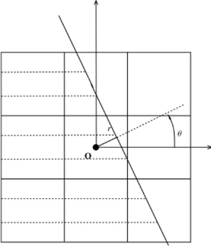
The first and main example directly comes from the VOF literature [10, 36, 31, 27]. For small mesh sizes, regular interfaces between fluids are asymptotically straight lines: that is why we consider only the latter limit case in this section. This example has a pedagogical virtue, and other cases will be variations around this theme. Straight lines
Iθ,rpx1, x2q “ cos θx1` sin θx2´ r, (4)
are described by 2 parameterspθ, rq P r0, 2πq ˆ R`, as illustrated in Figure 1.
θ O
r
Figure 1: Description of the parameterspθ, rq for straight lines.
The straight line delimits two half planes
P´“ tIθ,rpx1, x2q ă 0u and P`“ tIθ,rpx1, x2q ą 0u .
The intersection of square cells Ci, jwith the first half planetIθ,rpx1, x2qu ă 0 yields the volume fractions
αi j“
ż Ci jXP´
dx1dx2
which depend on the parameters θ and r. By definition the volume fractions are normalized between 0 and 1, that is αi j P r0, 1s.
Considering the other half plane P`would result in calculating 1´ αi j instead of αi j. To construct the inputs, we decide of a
certain blockp2N ` 1q ˆ p2N ` 1q of cells, symmetric with respect to the central cell, and gather the volume fractions in one
vector
α“ pαi, jq´Nďi, jďN P r0, 1sp2N`1q
2
Ă Rp2N`1q2. With these notations, the function D is
Then one has to decide the output which might be the periodic angle θ P r0, 2πq in this example. However forcing periodicity is not in the default implementation in Keras-TensorFlow. Therefore it is better for implementation purposes to work with 2
outputs which are the componentspcos θ, sin θq of the direction, because the 2π periodicity of the angle is naturally taken into
account and this procedure is easy to generalize in 3D. So our function E is
Epθ, rq “ pcos θ, sin θq . (6)
By construction the outputs are also normalized. For this exampleppar, in, outq “ p2, p2N ` 1q2,
2q.
3.3. Basic properties of ML methods
To have a self-contained presentation, we summarize hereafter the basic mathematical features which are used to construct the function F defined in (2-3). More theoretical material is proposed in the appendix to explain the good properties of ML algorithms for our purposes.
3.3.1. Functions
ML frameworks make use of high level recursive numerical functions, and three basic functions are sufficient to construct the function F.
Linear algebra. Functions like y“ WX ` b are implemented for X P Rn, WP Rmˆnand bP Rm.
Non linearity. Some non linear functions are implemented for x P R, such as the sigmoid σpxq “ p1 ` expp´xqq´1 or the
rectified linear unit (ReLU) function Rpxq “1
2px ` |x|q “ maxp0, xq.
Recursivity. Recursive calculations like W2RpW1X` b1q ` b2or R`W2RpW1X` b1q ` b2˘are implemented.
These functions can be used to construct other functions like maxpa, bq “ a ` Rpb ´ aq and minpa, bq “ ´ maxp´a, ´bq “
a´ Rpa ´ bq. Many more linear and non linear functions (convolution neural network, maxpool, . . . ) are also implemented
in Keras-TensorFlow [6, 33]. Once a combination is chosen, the structure of the function F is known. For example a
func-tion with one hidden layer (parameters W1, b1) is FpXq “ W2R
pW1X
` b1
q ` b2
, a function with two hidden layers is
FpXq “ W3pR`W2RpW1X` b1q ` b2˘` b3, and so on and so forth. A key feature of modern ML software is the
calcula-tion of the coefficients W1, b1, . . . of a function F which is represented or approximated within the above structure. This is
performed by optimization of a functional which encodes (2-3). This optimization uses stochastic gradient descent with auto-matic differentiation for the calculation of the gradient. The ReLU function R is piecewise differentiable, its derivative is the Heaviside function almost everywhere: it allows symbolic differentiation with the chain rule to calculate the first gradient of functions defined recursively. Comprehensive references can be found in [6, 33].
3.4. Elementary VOF advection and ML
We detail in this Section two simple reasons why the non linear ReLU function R is one of the best, better than a sigmoid σ, for application to VOF reconstruction on Cartesian grids.
The first reason is that many Finite Volume schemes with second-order accuracy use limiters as
minmodpa, bq “
"
0 for abď 0,
minp|a|, |b|qsignpaq for abą 0.
One has the formula minmodpa, bq “ Rpa ´ Rpa ´ bqq ´ Rp´a ´ Rpb ´ aqq which shows that limiting techniques are also prone
to be rewritten recursively with the ReLU function R. In view of the mathematical theory of hyperbolic equations [18], it is also
instructing to remark that the ReLU function R is deeply connected to Kruzkov entropies ηkpxq “ |x ´ k| “ Rpx ´ kq ` Rpk ´ xq.
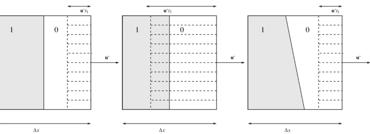
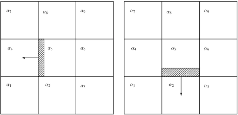
The second reason is based on the following geometric observation. Consider Figure 2 where, on the left and central parts,
an interface splits a 2D cell with area ∆x2in 2 pieces. In terms of a reconstructed volume fraction, it corresponds to a function
αpx, yq “
"
1 for 0ă x ă γ∆x, 0ď γ ď 1,
0 for γ∆xă x ă ∆x.
Consider that a velocity u˚ą 0 is given and compute the flux at the right boundary during a time 0 ă ∆t ď ∆x
u˚ fp∆tq “ ż∆x y“0 ż∆x x“p1´βq∆x αpx, yqdxdy, β“u ˚∆t ∆x .
u˚t 1 ∆x u˚ 1 0 u˚t 2 ∆x u˚ 1 0 u˚t 1 ∆x u˚ 1 0
Figure 2: Description in a square cell of the swept region delimited by a moving interface. The swept region (in dashed) depends on the time t. In gray the value of the indicatrix function is 1, in white the value is 0. On the left part, the time is t1“4u∆x˚: the flux is f1“ 0 and the mean volume fraction is ∆xf21{4 “ 0. On
the center part, t2“4u3∆x˚: the flux is f2“∆x
2
4 and the mean volume fraction is f2
3∆x2{4“13.
An exact calculation yields fp∆tq “ ∆x2R
pβ ´ γq that is
fp∆tq “ ∆xR pu˚∆t´ γ∆xq . (7)
One recognizes the SLIC method [26, 27] or the antidiffusive scheme [23]. The formula (7) shows that the rectified linear unit function has the ability to be exact for some elementary VOF procedure. On the right part of the Figure, the interface has an angle
and a reasonable approximation is fp∆tq « ∆xα1Rpu˚∆t´ γ1∆xq ´ ∆xα2Rpu˚∆t´ γ2∆xq with α1, α2, γ1and γ1conveniently
chosen.
More arguments in favor of using the function R are in the recent works [9, 35]. These basic observations are the reason why we use only the ReLU function R in our tests, because we believe it is more adapted.
3.5. Application to ML angle reconstruction for straight lines
We address the interpolation features of Keras-TensorFlow and measure its ability to construct the function F for the recon-struction of the angle. A reference, but with a completely different method, is the ELVIRA algorithm [27] which is exact for the reconstruction of the angle for straight line interfaces.
This section is a continuation of the pedagogical example Section 3.2. The vectors in the ML dataset B are constructed as
follows. The distance to the origin, parameter r, is sampled uniformly in the rangep´0.5?2, 0.5?2q (here 41 values): so the
central cell is always crossed by the interface (even if at a corner of the cell in the extreme case). We sample the angle θ uniformly
inr0, 2πq every degree (that is 360 values). It yields nθˆ nrvectors in R9for 3ˆ 3 blocks, or in R25for 5ˆ 5 blocks. The volume
fractions are calculated with numerical integration in 2D (Nquadraˆ Nquadra points with Nquadra “ 100). The parameter Nquadrais
the number of integration point per dimension and it yields a quadrature error ǫquadra «
1
Nquadra “ 1%. (8)
It produces cardpBq vectors ziP Rpar. Then we apply the function D in (5) which calculates volume fractions: it yields cardpBq
vectors
pXiq1ďiďcardpBq, Xi“ Dpziq P Rin, in“ p2N ` 1q2.
We also apply the function E in (6) which calculates the normal to the interface: it yields cardpBq vectors
pyiq1ďiďcardpBq, yi“ Epziq P Rout, par“ 2.
Systematically, 80% of the data belongs to the training dataset while 20% of the data belongs to the test dataset: this choice is made at random. At the end of this stage we have a dataset for training
Btrain“ " pXi, yiq, 1 ď i À 4 cardpBq 5 *
and a dataset for testing Btest“ " pXi, yiq, 1 ď i À cardpBq 5 * .
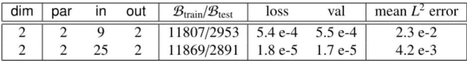
We use a dense two-layer ML reconstruction: the number of neurons of the dense hidden layer is systematically equal to the size of the inputs (parameter in), for example in=9 neurons for the first line of Table 1. Theoretically we postulate that an approximation formula (see Appendix A) holds for the function
F: RinÝÑ Rpar
XÝÑ y “ FpXq
and we let Keras-TensorFlow find weights such that the least square error is quasi-minimized, in the context of implementation with batches, 1 cardpBtrainq cardÿpBtrainq i“1 |yi´ FpXiq|2. (9)
In all our tests, we use the default parameters. The stochastic gradient descent runs with the Adam-optimizer [22]. Here the batch size is 128. The number of epochs is 200.
It yields Table 1 where the third column is the number of training/validation data. The loss error defined by (9) is in column 5. The validation error (equal to (9) but with the dataset for testing instead of the dataset for training) is in column 6. We observe that they are of the same order. Actually in all training sessions, we have observed that the loss error and the validation error are systematically of the same order, which is hopefully the sign that no overfitting or underfitting is attached to the ML treatment of our data. We will not report anymore on this feature in the rest of the paper, since it is not a restriction.
The last column is the mean value of the L2error on the test data (equal to the square root of the error-validation). Clearly,
the direction vector is recovered with an error around 2%. The results are promising.
dim par in out Btrain/Btest loss val mean L2error
2 2 9 2 11807/2953 5.4 e-4 5.5 e-4 2.3 e-2
2 2 25 2 11869/2891 1.8 e-5 1.7 e-5 4.2 e-3
Table 1: Accuracy of the direction vectorpcos θ, sin θq for straight lines in 2D.
Many tests have been performed with the 2D data1: it has been observed that the L2 error can be decreased by increasing
the number of dense hidden layers (that is by increasing the quality of the interpolator). But here the gain is marginal. Indeed
making the additional hypothesis that the predicted direction has norm equal to one, the mean L2 error, when it is small, scales
like mean L2error « d 1 cardpBtestq řˆˇˇˇ
ˇ cos θsin θtruetrue ´
ˇ ˇ ˇ
ˇ cos θsin θpredicpredic
˙2 « c 1 cardpBtestq ř ` θtrue´ θpredic ˘2 “ ǫθ.
In 2D, it means ǫθis around 1% in relative unit
ǫθ« 1%. (10)
Considering that the numerical integration (8) has itself a maximal error ǫquadra of the same order, it is probably meaningless to
increase the accuracy, without increasing the accuracy of the ML dataset (by increasing the accuracy of the numerical integration).
1A similar test has been performed in 3D. It is a confirmation in our framework of the 3D results in [28]. Now blocks are 27 cells or 125 cells, and the angles
pϕ, θq P r0, 2πq ˆ r0, πs which determine the planes are sampled quasi-uniformly to avoid over sampling near the poles. The numerical integration is uniform (Nquadraˆ Nquadraˆ Nquadrapoints with Nquadra“ 50). The results for the recovery of the direction vector psin θ cos ϕ, sin θ sin ϕ, cos θq for planes in 3D are
displayed below and they are quantitatively the same as in 2D.
dim par in out Btrain/Btest loss val mean L2error
3 4 27 3 11313/2781 1.e-3 1.e-3 3.2e-2 3 4 125 3 11272/2822 1.3e-4 2.9e-4 1.7e-2
4. More general geometries and definition of a dimensionless VOF-ML flux
In the following, we parametrize the geometry by arcs of circle and corners which are assembled to describe interfaces more general than just straight lines, even if the principles are exactly the same. We also explain how to define and train the normalized original VOF-ML flux which will be used in the remap stage of the compressible solver.
4.1. Arcs of circle
We refer in [28] for the ML modeling of interfaces between incompressible fluids. Our implementation is slightly different because we ask that the modeling of curved lines degenerates to the one of straight lines if applied to a mesh with smaller and smaller mesh size (it allows natural mesh convergence tests).
r θ d A O L
Figure 3: Description of the parameterspθ, r, d, Lq for arcs of circle.
Consider the circle of Figure 3: the center is
A“ rpcos θ, sin θq ` dp´ sin θ, cos θq ´ Lpcos θ, sin θq,
the radius is Lě 0 and the offset in the direction perpendicular to pcos θ, sin θq is d P R. Take a point x “ px1, x2q P R2inside
the disk of radius L, that is|x ´ A|2ă L2
. The expansion is
px1´ r cos θ ` d sin θ ` L cos θq
2
` px2´ r sin θ ´ d cos θ ` L sin θq
2
ă L2.
Cancellation of some terms yields 2Lpcos θx1` sin θx2´ rq ` px1´ r cos θ ` d sin θq
2 ` px2´ r sin θ ´ d cos θq 2 ă 0, that is Iθ,rpx1, x2q ` 1 2L ”
px1´ r cos θ ` d sin θq2` px2´ r sin θ ´ d cos θq2
ı ă 0.
Using a rescaling of all lengths x1, x2, r, d, L by a factor which corresponds to the mesh size ∆x, one gets
Iθ,rpx1, x2q ` 1 2ν ” px1´ r cos θ ` d sin θq 2 ` px2´ r sin θ ´ d cos θq 2ı ă 0, (11)
where the factor is ν“ ∆x
L ą 0. For small mesh size ∆x, the continuous limit ν Ñ 0 recovers the equation (4) of straight lines
2.
Taking par“ 4 and in “ p2N ` 1q2as before, the function D : RparÑ Rinis defined by Dpθ, r, d, Rq “ α. The function E will
be described in Section 4.3 in formula (12).
2If one desires to capture instead the small radius limit, that is LÑ 0`, it is better to rescale the equations. Then take σ“1 ν “
L
∆xand the parametrization
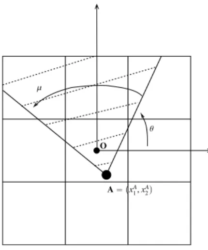
4.2. Corners
The interfaces described above are smooth and so are not satisfactory for the local modeling of interfaces which are not C1
but only Lipschitz, such as the cross test problem and the Zalezak test problem which will be considered in the numerical section. For such test problems, normal vectors at the interfaces have points of discontinuities: these points are called corners or corner
points in this work. Consider the illustration in Figure 4. Straight lines correspond to µ“ π (it is a degenerate case), right angles
correspond to µ“ π
2 and µ“ 3
π
2 and acute angles correspond to the other values of µ. The corner is denoted as A“ px
A
1, x
A
2q.
Actually this modeling of corners allows also to model straight line interfaces, it is sufficient either to take µ“ π or to sample A
outside of the block with an additional condition on the aperture of the corner.
A“ pxA 1, xA2q
µ
θ O
Figure 4: Description of the parameterspθ, µ, xA
1, xA2q for corners.
With these notations, one has par“ 4 and in “ p2N ` 1q2. The function D : Rpar Ñ Rinis defined by Dpθ, µ, xA
1, x
A
2q “ α.
The function E is described in the next Section 4.3 in formula (12).
4.3. Definition of a dimensionless VOF flux and adapted inputs
The function f in (7) used for the pedagogical case of straight lines is not normalized. For normalization reasons, it is better to consider the average flux which is the flux divided by the area of the swept region
gp∆tq “ fp∆tq
p1 ´ βq∆x2. (12)
This quantity is normalized in the sense that, on the one hand gp∆tq can be evaluated in function of the normalized quantities
βP r0, 1s and γ P r0, 1s, and on the other hand gp∆tq P r0, 1s under the CFL condition u˚∆t
∆x P r0, 1s. Other tests performed for
the ML reconstruction of fp∆tq show a loss of accuracy for small velocity or for small Courant number: it was expected because
fp∆tq P r0, ∆xu˚∆ts is systematically small for small ∆t; on the contrary gp∆tq is much less sensitive to small ∆t. For all these
reasons, we advocate using g instead of f as output for VOF flux reconstruction. This gives the function E“ gp∆tq that will be
used from now on with out“ 1.
The reconstruction of the parameters of the different types of interfaces is not sufficient for the remap stage of CFD calcula-tions. Indeed, even with an accurate reconstruction of these values, one must still construct the flux at the cell face. Therefore, to have a satisfactory ML modeling of the flux, we enlarge by one the size of the inputs. The new input is the rescaled velocity which scales like a non dimensional Courant number
β“ u˚∆t{∆x P r0, 1s.
We add it to the volume fractions, so the function D maps the parameters to a vector made of the volume fractions plus β
Dpinterface parametersq “ pα, βq P Rp2N`1q2`1. (13)
For example for a 3ˆ 3 block, the size of the inputs is now in “ 1 ` 9 “ 10. The output size is out “ 1: the output is the
dimensionless outgoing flux
g“1 β ż 1 2 1 2´β ż 1 2 ´1 2 αpx, yqdxdy P r0, 1s (14)
where α is the indicatrix function, as described in (12). It yields the function E
Epinterface parametersq “ g P R. (15)
4.4. Validation of the VOF-ML flux for straight lines
Redoing the tests of Table 1 for N “ 3 and N “ 5, the dimensions are now par “ 2, in “ 1 ` p2N ` 1q2and out“ 1. The
size of the ML dataset is 100ˆ 360 ˆ 41. The batch size is 16 ˆ 1028. The number of epochs is still 200. We use 2 dense hidden
layers: a first one with 4ˆ in neurons, a second one with 2 ˆ in neurons. The results are in Table 2. One observes that the results
in the last column are even slightly better than in Table 1. It validates the use of the mean flux as the output.
dim par in out Btrain/Btest loss val mean L2error
2 2 10 1 1192451/298309 7e-5 7.1 e-5 9.8e-3
2 2 26 1 1193738/297022 8.8e-5 9.4e-5 6.5e-3
Table 2: Accuracy of the VOF-ML flux for straight lines.
At the end of this procedure, all the geometry (interface reconstruction, numerical integration of indicatrix functions in normalized cells, numerical integration of the flux) is offline. That is, it is considered only in the Python-Keras-TensorFlow stage of the calculation chain.
4.5. Construction of ML datasets and accuracy of the VOF-ML flux for general geometries
The construction of the ML datasets relies so far on uniform sampling of all parameters. This was possible because the number of parameters was small, equal to 2 in this example.
But we need more parameters to describe complex interfaces like arcs of circles and corners, so uniform sampling is no more possible because the number of configurations would blow up. That is why we decided, quite arbitrarily, to keep the uniform sampling of the angle θ and of the rescaled velocity β, and to take random values for all other parameters. Now the size of the
ML dataset is nθˆ nβˆ 2 ˆ P: the factor 2 is because we systematically take the contrasted values (rα“ 1 ´ α) and the extra
factor P guarantees that the same value of the parameters θ and β are used P times while the other parameters are randomized. The sampling of the rescaled velocity β is equal to the sampling for the numerical integration, because it is convenient for
implementation purposes, that is nβ“ Nquadra.
The result for the reconstruction of the flux for arcs of circle (Section 4.1) are in Table 3, where nθ“ 8 ˆ 360, nβ“ Nquadra “
100, P“ 3 and we randomize the parameters r ď 2?2, dď
b
N`12 and Lď 2?2. The error (last column) is still considered
small enough.
dim par in out Btrain/Btest loss val mean L2error
2 5 10 1 1395790/349490 4.2e-5 4e-5 6.3e-3
2 5 26 1 1395422/349858 3.1e-5 4.2e-5 6.5e-3
Table 3: Accuracy of the VOF-ML flux for arcs of circle.
Finally we consider the corner configuration of Section 4.2. We take nθ “ 24 ˆ 360 uniformly distributed angles. We take
nβ“ 100 values of β which are uniformly distributed. We double the results (taking the negative value α Ð 1´α and β Ð 1´β).
The parameters xA, yAare taken random in the squarer´3{4, 3{4s for in “ 10 and in the square r´5{4, 5{4s for in “ 26 . The
parameter µ takes two different values π
2 and
3π
2 at random, it models only right angles. The results are displayed in Table 4.
It seems the 3ˆ 3 block has more difficulty to recover the solution, even if the accuracy is still of the same order as previous
accuracies. It is probably related to some lack of invertibility of the function D for 3ˆ 3 blocks (a topic already evoked at the
end of Section 3.1). It is also probably related to the lower regularity of this type of Lipschitz interfaces. 5. Inference of the model in a C++ code
Now that ML datasets are built with various parameters, and that the training and testing are performed, it remains to pass the model to a C++ code for the inference, i.e. the F function call.
dim par in out Btrain/Btest loss val mean L2error
2 5 10 1 1396604/348676 1.9e-3 2.1e-3 4.5e-2
2 5 26 1 1396744/348536 1.6e-4 2.2e-4 1.5e-2
Table 4: Accuracy of the VOF-ML flux for corners (right angles).
The software keras2cpp offers the ability of calling the function many times on tensors (which are arrays)
TinputP RNtensorˆin. (16)
The size of the rectangular tensor T is Ntensorˆ in where Ntensoris the number of fluxes that one desires to calculate and in is the
size of the inputs. The function F then returns a tensor
Toutput“ F pTinputq P RNtensorˆout (17)
where out is the size of the outputs (actually equal to 1 in our case). This procedure allows a natural acceleration which is highly
profitable for performance: a typical mean value of a call to F is between 10´5s and 10´4s, see the end of Section 8.
At the end of this stage, one has a function F callable in C++ which realizes the task (2-3) for the considered dataset: the output is the dimensionless flux (12).
6. Implementation in a Finite Volume solver
We provide some important details of the implementation of the method within a Finite Volume solver.
6.1. Preservation of natural symmetries
Calculations on a Cartesian mesh should in principle respect natural symmetry principles, when they are available. Moreover
the accuracy of the ML interface reconstruction is achieved with an accuracy« 1% for the reason explained above. So any loss
of symmetry can induce important discrepancies. The situation is different for incompressible fluid flow where the curvature
of bubbles is recovered within an error of 10´6 with ML algorithms [37]. We particularize 3 different symmetries, and the
consequences for the implementation of the VOF-ML scheme.
Rotational symmetry on a Cartesian mesh. The scheme must be invariant when a rotation of angle π{2 is applied. This is
easy to obtain with a convenient ordering of the volume fractions. This principle is already used in standard Finite Volume implementations [24][Chapter 24], so there is no need to describe further. See Figure 5 for an illustration.
α2 α4 α5 α6 α1 α3 α9 α8 α7 α1 α4 α5 α6 α3 α9 α8 α7 α2
Figure 5: A rotational symmetry is described for a 3ˆ 3 block. On the left the call is Fpβ, α1, α2, α3, α4, α5, α6, α7, α8, α9q. On the right it is Fpβ1, α
3, α6, α9, α2, α5, α8, α1, α4, α7q where the ordering of the volume fractions is the same up to a rotation. A similar procedure is used for calculation
of the flux across the right boundary and the top boundary.
Mirror symmetry. Consider transport in the left direction, as in Figure 5. Let Y “ pα1, α2, α3, α4, α5, α6, α7, α8, α9q and
con-sider its rearrangement ΠY “ pα7, α8, α9, α4, α5, α6, α1, α2, α3q, where the bottom line components α1, α2, α3 are
ex-changed with the top line components α7, α8, α9. The function should satisfy the mirror symmetry Fpβ, Yq “ Fpβ, ΠYq,
but such a symmetry is not guaranteed by our construction. So we force it by implementing
Fmirpβ, Yq “
1
A similar treatment is applied for the left-right mirror symmetry.
Numbering symmetry. It means that the result should be the same if we exchange the role of material 1 and material 2 in the
model, that is if we exchange a1and a2. Mathematically, it can be described by considering the vector e“ p1, . . . , 1q and
the function ΛY“ e ´ Y. We note the commutation ΠΛ “ ΛΠ. The numbering symmetry corresponds to the property
Fpβ, ΛYq “ 1 ´ Fpβ, Yq.
Since the construction does not guarantee this property, we force it by implementing
Fnumbpβ, Yq “
1
2pFpβ, Yq ` 1 ´ Fpβ, ΛYqq .
The scheme which is implemented satisfies all symmetries by using
Fpβ, YqMLVOF“1
4pFpβ, Yq ` Fpβ, ΠYq ` 1 ´ Fpβ, ΛYq ` 1 ´ Fpβ, ΛΠYqq . (18)
This flux is called the VOF-ML flux in the rest of this article3.
6.2. Preservation of natural bounds
It is expected that the VOF-ML flux (18) can violate natural bounds like 0ď a1ď 1, since no such considerations have been
used so far. Of course, any kind of a posteriori method can be used to recover the maximum principle. In this work we use a simple a priori bound which is well adapted to directional splitting implementations. Essentially we constraint the flux so that no negative volume or mass is created.
Consider a square cellp0, ∆xq2
with initial volumes 0ď V1“ a1∆x2and 0ď V2“ a2∆x2with a1` a2“ 1. Assume a flux
a˚1 is applied on one side for a velocity u˚ą 0, and disregard the flux on the other side. The remaining volumes at the end of the
time step will be V1“ V1´ ∆xpa˚1∆xu˚q and V2“ V2´ ∆xpa2˚∆xu˚q where a˚2 “ 1 ´ a˚1. Note that V1` V2ă ∆x2, but this is
not the important point. The conditions V1ě 0 and V2ě 0 yield two inequalities a˚1 ďu∆x˚∆ta1and 1´ a˚1 ďu∆x˚∆tp1 ´ a1q which
are summarized in 1´ ∆x u˚∆tp1 ´ a1q ď a ˚ 1 ď ∆x u˚∆ta1.
This double bound is systematically added in our implementation of the VOF-ML flux. It yields a non negativity principle, which transfers into a maximum principle for the volume fractions (and mass fractions as well). In practice we check if the
VOF-ML flux (18) belongs to the interval“1´ ∆x
u˚∆tp1 ´ a1q,u˚∆x∆ta1
‰
: if it is in the interval we do nothing; if it is outside the interval, we replace the value of the flux with the nearest extreme value in the interval, which is equal either to the lowest value
1´ ∆x
u˚∆tp1 ´ a1q or to the highest oneu∆x˚∆ta1.
6.3. Hybridation of the VOF flux
VOF schemes are often used in combination with other numerical techniques [27, 4]. For example a VOF interface recon-struction technique can be used near the interface, while a more traditional Finite Volume scheme may be used away from the interface. This is why it is probably better to conceive that VOF-ML schemes must be hybrid ones. Hybrid schemes have also the virtue that, in principle, the higher numerical cost of sophisticated VOF schemes contributes to the total cost only for cells near the interface.
The schemes developed in this article for test purposes are hybrid schemes. Various sensors have been tested, but the simplest
one is retained. A small threshold value ǫflagą 0 is taken and one checks at the beginning of every iteration and for all cells if a1
is in between ǫflagand 1´ ǫflag:
if ǫflagď a1ď 1 ´ ǫflagùñ the cell is flagged.
If the cell is flagged, one uses the VOF-ML flux (18): in the other case, we use another much cheaper method; in the Euler2D code, the anti-dissipative SLIC/Downwind flux is available, it is cheap and with strong anti-dissipative properties [23]. Consid-ering that the quadrature error and average accuracy at the end of the training session are of the order of 1%, we take a slightly greater value
ǫflag“ 2 10´2. (19)
With this value, all thresholds (8), (10) and (19) have the same magnitude. It reflects a kind of compatibility of the whole chain of calculation.
3The cost of this procedure is 4 times the cost of one individual call to the function F. On a Cartesian grid in dimension d with m different materials, the cost
6.4. An additivity principle for the ML datasets
The additivity principle states that the ML dataset used for computing a given profile must be the union (or the addition) of ML datasets dedicated to different local features of the profile. In mathematical words, it means the ML dataset uses different
functions D1, D2, . . . , but the same function E, and that the function F is the best that ML can construct such that
FpDipzqq « Epzq for all z P Rparand for all i“ 1, 2, . . . (20)
This additivity principle is more a "good practice" requirement, and no theory is available so far. However its efficiency is
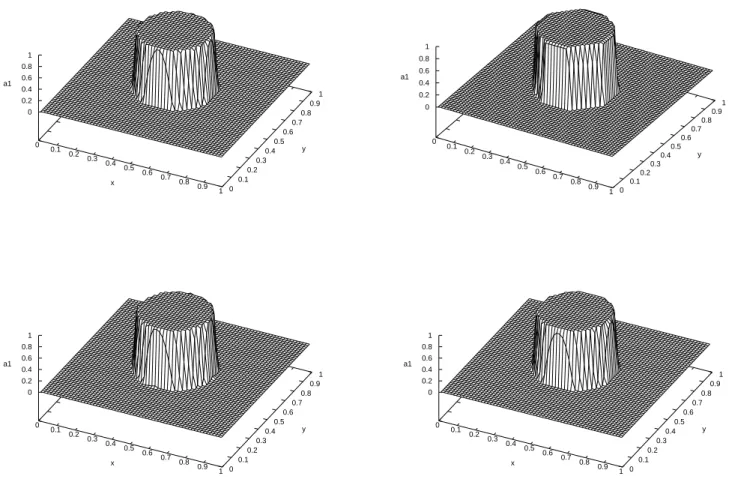
0 0.1 0.2 0.3 0.4 0.5 0.6 0.7 0.8 0.9 1 x 0 0.1 0.2 0.3 0.4 0.5 0.6 0.7 0.8 0.9 1 y 0 0.2 0.4 0.6 0.8 1 a1 0 0.1 0.2 0.3 0.4 0.5 0.6 0.7 0.8 0.9 1 x 0 0.1 0.2 0.3 0.4 0.5 0.6 0.7 0.8 0.9 1 y 0 0.2 0.4 0.6 0.8 1 a1 0 50 100 150 200 250 300 0 5 10 15 20 25 30 Flagged cells x 0 20 40 60 80 100 120 0 5 10 15 20 25 30 Flagged cells x
Figure 6: Value of volume fraction a1at time t“ 0.1. Top left: the ML dataset has only straight lines. Top right: the ML dataset is made of straight lines and
corners, following the addition principle. Bottom: the number of flagged cells versus number of time steps.
illustrated by the following simple numerical experiment. Consider the advection of a square. Locally the square is made of straight lines and corners. In the top left part of Figure 6, a simulation is displayed where the ML training is done with a dataset
with straight line profiles on 5ˆ 5 blocks. It is clear that the numerical procedure is efficient for the capturing of straight lines,
but the accuracy is very poor at corners. On the contrary, on the top right part of the Figure, the ML dataset is the addition of two ML datasets dedicated to straight lines and corners. Clearly, the overall accuracy is correct.
On the bottom of Figure 6, the number of flagged cells is plotted in function of the number of iterations in time. On the left part, the number of flagged cells increases linearly. It renders the computation inefficient and inaccurate. On the right part of the Figure, with the good resolution ML dataset (that is with straight lines and corners), the number of flagged cells is bounded uniformly with respect to the iterations.
Not only the ML algorithm is able to find good parameters for the advection of straight lines and corners separately, but also it is able to interpolate smoothly from case to the other. More generally we have observed in all our calculations that this principle is true:
7. A simple bi-material hydrodynamics model
Numerical tests of the VOF-ML flux have been performed in the Euler2D code developed by F. Lagoutière [23] that is described below.
In its basic setting, it uses a first-order accurate Lagrange+remap Finite Volume scheme with directional splitting [4] on a 2D Cartesian grid. The global scheme is conservative for masses, total momentum and total energy, and is endowed with strong stability properties based on entropy inequalities [23]. It solves a bi-material compressible Euler model
$ ’ ’ & ’ ’ % Btpρc1q ` ∇ ¨ pρc1uq “ 0, Btpρc2q ` ∇ ¨ pρc2uq “ 0, Btpρuq ` ∇ ¨ pρu b uq ` ∇p “ 0,
Btpρeq ` ∇ ¨ pρue ` puq “ 0.
The additivity of mass fractions, specific volumes (1{ρ “ τ) and internal energies is assumed
$ & % 1“ c1` c2, τ“ c1τ1` c2τ2, e“ c1ǫ1` c2ǫ2`12|u|2.
We use perfect gas pressure laws
p1“ pγ1´ 1qρ1ǫ1and p2“ pγ2´ 1qρ2ǫ2.
For γ1 “ γ2, the model degenerates to a mono-fluid or mono-material model. Truly bi-fluid or bi-material configurations
correspond to γ1 ‰ γ2. The closure (that is the global pressure p) is calculated in accordance with, either the
iso-pressure/iso-temperature model (p1“ p2, T1“ T2, ε1“ Cv1T1and ε2“ Cv2T2), or the iso-pressure/iso-δQ model
p1“ p2, Dtǫ1` p1Dtτ1“ Dtǫ2` p2Dtτ2.
The iso-pressure/iso-δQ model is our preference because the quality of the results is often better, but its implementation is non trivial because this closure model is non conservative. On the other hand the mathematical analysis of the iso-pressure/iso-temperature model is simpler, moreover its implementation is easier and the code is more robust: these are valuable features for
comparisons. We will show results with both closures. If the initial data is constant pressure ppt “ 0, xq “ prefand constant
velocity up0, xq “ uref, then the exact solution of the model (whatever the closure) is provided by the solution of pure advection
at velocity uref. The volume fractions are related to the mass fractions and specific volumes
a1“
c1τ1
τ and a2“
c2τ2
τ “ 1 ´ a1.
The boundary conditions can be periodic, neutral or wall conditions. Periodic boundary conditions are required for pure advection test cases. Two advection schemes are available in the Euler 2D for the remap stage. The first one is the first-order accurate upwind scheme which has poor accuracy for interfaces. The second one is the downwind scheme under upwind constraints [23]: it is similar to the SLIC algorithm [26] and will be referred to as the SLIC/Downwind scheme. The other details of such a code are standard, we refer to [23, 4].
8. Numerical results
Here we report on the accuracy of the new VOF-ML procedure, by considering basic test problems of the literature calculated within Euler2D. We distinguish pure advection and shock problems.
In order to explain what is needed for the calculation of a given type of interface, we consider VOF-ML fluxes issued from different datasets. For the Zalezak notched circle problem shown in Figure 9, the dataset is complete in the sense that it contains arcs of circles, right corners and corners with angle. In the appendix, a dedicated and somewhat artificial dataset is specially
designed for the Trifolium test problem. An accurate model callable with keras2cpp for a 5ˆ 5 block trained with a ML dataset
8.1. Advection test cases
The initial data is pressure equilibrium and the vectorial velocities are the same in all cells u “ uref “ pa, aq with a “ 1.
We use periodic boundary conditions. The domain of calculation is a square with characteristic length equal to 1. The exact
solution at time t“ 1 is also the initial solution. The schemes use directional splitting. With an appropriate choice of the initial
data, the sound speed c is smaller than the material velocity in both dimension, that is că 1. The indicated Courant number is
CFL“ a∆t
∆x. In our tests, the Courant number varies between 0.1 to 0.6 in order to explore the sensibility of the algorithm. It
must be noticed that Courant numbers too close to 1 are of less interests since our advection scheme becomes perfect at the limit. Also the Courant number is one parameter in the vector of inputs (parameter β): since the training session can be interpreted as an interpolation procedure, it is expected that the quality of the interpolation is smaller at the boundary of the domain of inputs (in phase space), so for Courant numbers close to 0 or to 1. For Courant numbers close to 1, this phenomenon probably mitigates the fact that an upwind advection scheme is perfect at the limit.
8.1.1. The cross
This is an extension of the square test problem displayed in Figure 6. The Courant number is 0.4. The ML dataset is made of
curved lines and corners. Actually when ν“ 0, the curved lines (arcs of circle) dataset contains the straight lines dataset. So the
accuracy for straight lines description is a priori as good as it is with only straight lines in the dataset.
0 0.1 0.2 0.3 0.4 0.5 0.6 0.7 0.8 0.9 1 0 0.1 0.2 0.3 0.4 0.5 0.6 0.7 0.8 0.9 1 0 0.2 0.4 0.6 0.8 1 0 0.1 0.2 0.3 0.4 0.5 0.6 0.7 0.8 0.9 1 0 0.1 0.2 0.3 0.4 0.5 0.6 0.7 0.8 0.9 1 0 0.2 0.4 0.6 0.8 1 0 0.1 0.2 0.3 0.4 0.5 0.6 0.7 0.8 0.9 1 x 0 0.1 0.2 0.3 0.4 0.5 0.6 0.7 0.8 0.9 1 y 0 0.2 0.4 0.6 0.8 1 a1 0 0.1 0.2 0.3 0.4 0.5 0.6 0.7 0.8 0.9 1 0 0.1 0.2 0.3 0.4 0.5 0.6 0.7 0.8 0.9 1 0 0.2 0.4 0.6 0.8 1
Figure 7: Value of volume fraction a1at time t“ 1. Top left initial data (also equal to final data). Top right, SLIC/Downwind scheme. Bottom left, blocks are
3ˆ 3. Bottom right, blocks are 5 ˆ 5.
In the ML dataset we oversample the corners (1163196 items, obtained with 4ˆ 18 ˆ 20 angles, only right angle corners
that is µ “ π{2 or µ “ 3π{2 only, and 10 different values of the corners positions) with respect to arcs of circle (348754 items,
obtain a satisfactory accuracy. The interpretation is that it counteracts the lower accuracy of corner reconstruction with respect to straight lines reconstruction (just compare the last column of Table 2 and 4). Here we use 5 dense layers in the neural network (meaning we use 5 levels of recursivity as described in Section 3.3.1).
The results are displayed in Figure 7. The results are good, in particular for the 5ˆ 5 blocks. Looking in more detail at the
top right part of the Figure where the result is computed with the SLIC/Downwind scheme available in the code [23], one sees large errors because the branches of the cross are not aligned. This is not observed with the VOF-ML scheme.
8.1.2. The disk
The disk is discretized on a 40ˆ 40 cells grid. The Courant number is 0.4. The results with 3 ˆ 3 blocks and 5 ˆ 5 blocks
are displayed in Figure 8. We also display the result obtained with the anti-dissipative scheme [23] which is over-compressive: it quickly captures an octagon instead of a disk. We use of course the ML dataset with arcs of circle. The results with the VOF-ML schemes are qualitatively accurate.
0 0.1 0.2 0.3 0.4 0.5 0.6 0.7 0.8 0.9 1 x 0 0.1 0.2 0.3 0.4 0.5 0.6 0.7 0.8 0.9 1 y 0 0.2 0.4 0.6 0.8 1 a1 0 0.1 0.2 0.3 0.4 0.5 0.6 0.7 0.8 0.9 1 0 0.1 0.2 0.3 0.4 0.5 0.6 0.7 0.8 0.9 1 y 0 0.2 0.4 0.6 0.8 1 a1 0 0.1 0.2 0.3 0.4 0.5 0.6 0.7 0.8 0.9 1 x 0 0.1 0.2 0.3 0.4 0.5 0.6 0.7 0.8 0.9 1 y 0 0.2 0.4 0.6 0.8 1 a1 0 0.1 0.2 0.3 0.4 0.5 0.6 0.7 0.8 0.9 1 x 0 0.1 0.2 0.3 0.4 0.5 0.6 0.7 0.8 0.9 1 y 0 0.2 0.4 0.6 0.8 1 a1
Figure 8: Value of volume fraction a1at time t“ 1 after one round turn. Top left, initial and final data. Top right, SLIC/Downwind scheme. Bottom left, blocks
are 3ˆ 3. Bottom right, blocks are 5 ˆ 5.
8.1.3. The Zalezak notched circle
We consider the advection of the Zalezak notched circle [27] tilted π
7 with respect to the mesh axis. The elevations are
displayed in Figure 9. The results with the SLIC/Downwind scheme are not accurate since the disk is transformed into a polygon
(as for the disk). The results calculated with a 5ˆ 5 block are better but a discrepancy is visible at one of the acute angles. But,
following the additivity principle, with right angles (µ“ π
2 or 3π
2) and acute angles (parameter 0ď µ ď π{8) in the dataset, the
0 0.1 0.2 0.3 0.4 0.5 0.6 0.7 0.8 0.9 1 x 0 0.1 0.2 0.3 0.4 0.5 0.6 0.7 0.8 0.9 1 y 0 0.2 0.4 0.6 0.8 1 a1 0 0.1 0.2 0.3 0.4 0.5 0.6 0.7 0.8 0.9 1 x 0 0.1 0.2 0.3 0.4 0.5 0.6 0.7 0.8 0.9 1 y 0 0.2 0.4 0.6 0.8 1 a1 0 0.1 0.2 0.3 0.4 0.5 0.6 0.7 0.8 0.9 1 x 0 0.1 0.2 0.3 0.4 0.5 0.6 0.7 0.8 0.9 1 y 0 0.2 0.4 0.6 0.8 1 a1 0 0.1 0.2 0.3 0.4 0.5 0.6 0.7 0.8 0.9 1 x 0 0.1 0.2 0.3 0.4 0.5 0.6 0.7 0.8 0.9 1 y 0 0.2 0.4 0.6 0.8 1 a1
Figure 9: Value of volume fraction a1at time t“ 1 after one round turn. Top left, initial and final data. Top right, SLIC/Downwind scheme: the notched circle
is transformed in a polygonal line as shown by the contour lines. Bottom left, blocks are 5ˆ 5, but the ML dataset does not have acute angles. Bottom right, blocks are 5ˆ 5, now the ML dataset has acute angles. The level set of the bottom right result is presented in Figure 10.
Below in Figure 10 we reproduce the contour 0.5 of the Zalesak profile at time t “ 1 and t “ 3. The same setting is used
(directional splitting, 15 cells in one radius). One observes that the VOF-ML scheme provides a good numerical rendering of the
corners and acute angles at t“ 1 even if a slight degradation is visible at t “ 3.
8.1.4. Convergence tests
It is instructive to perform convergence tests to get some guarantee of the good quality of these schemes with very fine meshes. It must be mentioned that the schemes being written in a Finite Volume framework, they are conservative for local masses, total impulse and total energy. We consider the advection of 2 smooth interfaces which are a disk and an ellipse. The
disk has a radius L“ 0.4. The equation of the ellipse is 2x2` y2“ L2. In the dataset the parameter r is carefully interpolated in
the intervalr0, 1.5?2s.
The results are displayed in Table 5 where we measure the difference between the initial data and the final data at time t“ 1
in the L1norm. One observes a low rate of convergence, however it is remarkable that, even on a coarse mesh, the level of error is
quite small in L1norm. Then, by refining the grid, the L1norm diminishes at a rate which is approximatively 1/2: that is doubling
the number of cells in every direction decreases the error by approximatively a factor ?2. This feature is clear on Figure 11.
Therefore one can consider that the new VOF-ML schemes have the attributes of a Finite Volume scheme: they are conservative
and converge in L1 norm at rate 1/2 for bounded variation (BV) data, that is the error scales like« CVOF´ML∆x
1
2. We refer
to [7, 12, 25] for estimates obtained in the context of standard numerical analysis and to [11] for an optimal estimate obtained
with probabilistic tools which shows convergence of Finite Volume schemes at a rate h12in L1 for initial data in BV. For the
0 0.1 0.2 0.3 0.4 0.5 0.6 0.7 0.8 0.9 1 x 0 0.1 0.2 0.3 0.4 0.5 0.6 0.7 0.8 0.9 1 y 0 0.1 0.2 0.3 0.4 0.5 0.6 0.7 0.8 0.9 1 x 0 0.1 0.2 0.3 0.4 0.5 0.6 0.7 0.8 0.9 1 y
Figure 10: Level set 0.5 of the advected Zalezak profile. Value of a1at time t“ 1 on the left and t “ 3 on the right. A small degradation of the quality of the
isoline at one internal corner is visible at t“ 3.
scheme. For the Upwind scheme, one observes convergence rate« CUpwind∆x
1
2, with a constant CUpwind« 600ˆCVOF´MLwhich
is much larger than the one of the VOF-ML scheme. For the SLIC/Downwind scheme, one observes a first order convergence
rate« CSLIC∆x: what is remarkable is that the constant CVOF´MLis so small so that the error of the SLIC/Downwind scheme for
the 480ˆ 480 very fine mesh is still greater than the error of the VOF-ML scheme on the coarse 30 ˆ 30 mesh.
In these tests, a rigorous protocol has been adopted. That is the parameters for the construction of the dataset for the 5ˆ 5
blocks are exactly the same as the parameters for the construction of the dataset for the 3ˆ 3 blocks. Also the training is done
with 5 000 epochs. As a result, on the Table and the Figure, the accuracy is very similar for 3ˆ 3 blocks and 5 ˆ 5 blocks. For
the finer mesh, the accuracy is slightly in favor of 5ˆ 5 blocks. With less rigorous protocols for the construction of datasets, the
comparison between 3ˆ 3 blocks and 5 ˆ 5 blocks is less clear. Here we see that the results are of equal quality between 3 ˆ 3
and 5ˆ 5 blocks. A simple explanation is that the boundaries are smooth and smooth curves tend to straight lines asymptotically
for small mesh size. Since straight lines are already well captured with 3ˆ 3 blocks it is not surprising that the gain offered by
5ˆ 5 is marginal here. On the contrary, if the interfaces are less regular as in Table 4, it must be reminded that 5 ˆ 5 blocks are
more accurate than 3ˆ 3 blocks.
0.001 100 disk: 3x3 ellipse: 3x3 disk: 5x5 ellipse: 5x5 theory: 1/2 theory: 1/2
Figure 11: Logarithmic plot of the L1error versus the number of cells. The data are from Table 5 and L1convergence at a rate« 1{2 is satisfied asymptotically.
8.2. Shock test problems
Test problems with shocks are often simpler than pure advection, since the interfaces coincide with contact discontinuities which are constrained by the dynamics of the equations (in particular they are often less singular). The time step is calculated
object block N1D L1 order order disk 3ˆ 3 30 0.001614 disk 3ˆ 3 60 0.001245 (0.3745) disk 3ˆ 3 120 0.000893 (0.4794) (0.4270) disk 3ˆ 3 240 0.000541 (0.7230) (0.6012) disk 3ˆ 3 480 0.000420 (0.3652) (0.5441) ellipse 3ˆ 3 30 0.001550 ellipse 3ˆ 3 60 0.001519 (0.0291) ellipse 3ˆ 3 120 0.001159 (0.3902) (0.2097) ellipse 3ˆ 3 240 0.000702 (0.7233) (0.5568) ellipse 3ˆ 3 480 0.000529 (0.4082) (0.5658) disk 5ˆ 5 30 0.001649 disk 5ˆ 5 60 0.000965 (0.7730) disk 5ˆ 5 120 0.000909 (0.0862) (0.4296) disk 5ˆ 5 240 0.000584 (0.6383) (0.3623) disk 5ˆ 5 480 0.000369 (0.6623) (0.6503) ellipse 5ˆ 5 30 0.002364 ellipse 5ˆ 5 60 0.001265 (0.9021) ellipse 5ˆ 5 120 0.001132 (0.1603) (0.5312) ellipse 5ˆ 5 240 0.000713 (0.6669) (0.4136) ellipse 5ˆ 5 480 0.000460 (0.6323) (0.6496)
Table 5: Convergence table. The 3ˆ 3 blocks and 5 ˆ 5 blocks are run with a VOF-ML scheme trained with 5 dense layers, with a large number of epochs (5 000 here) to reach accuracy of the training. For reasons explained in Section 8.3, the finer the mesh, the smaller the relative cost of VOF-ML with respect to the Finite Volume solver. In column 5, the L1numerical order of convergence is on“
log en´1´log en log 2 . In column 6, it is on“ log en´2´log en log 4 . 30 60 120 240 480 order Upwind 0.6633 0.4895 0.3565 0.2551 0.1818 « 0.5 SLIC/Downwind 0.0527 0.0352 0.0195 0.0108 0.0051 « 1
Table 6: Reference L1 norm of the error for the ellipse test case with the Upwind scheme and with SLIC/Downwind scheme. The best error with the
SLIC/Downwind scheme on the finest mesh is still much greater than the error of the VOF-ML scheme (in Table 5) on the coarsest mesh.
such that maxp|ux|, |uy|, cq∆x∆t ď 1. For the last test case where the sound speed takes high values, then the Courant number for
advection is small. For such simple shock problems, the SLIC/Downwind scheme already provides a satisfactory accuracy. Any
dataset made only with arcs of circles and with fine training is sufficient. Here the interfaces are smooth curves. We used 5ˆ 5
blocks. These problems also contribute to the validation of the VOF-ML flux for a non-trivial velocity field that contains some degree of vorticity beyond pure translation or pure solid body rotation.
8.2.1. 1D shock tube problem
We consider a symmetric 1D shock tube problem computed with the 2D code. The initial data come from the Sod shock tube
problem but with γ1‰ γ2
0.3ă x ă 0.7 : a1“ 1, a2“ 0, ρ1“ 1, p1“ 1, ux“ 0, uy“ 0, γ1 “ 1.6,
xă 0.3 or 0.7 ă x : a1“ 0, a2“ 1, ρ2“ 0.125, p2“ 0.1, ux“ 0, uy“ 0, γ2“ 1.4.
To have good resolution even with a first-order accurate acoustic Lagrangian Riemann solver, we use 1000ˆ5 cells. The Courant
number is 0.6. The results calculated with the iso-pressure/iso δQ model are displayed in Figure 12. The steepness of the contact discontinuity is perfectly captured both on the density profile and on the volume fraction profile. In particular the perfect right-left
symmetry of the profile is visible on the profile for a1.
8.2.2. 2D convergent shock problem
We consider a convergent mild shock bi-material test problem where γ1 “ 1.4, γ2 “ 1.6. The isobar-isothermal closure
0.1 0.2 0.3 0.4 0.5 0.6 0.7 0.8 0.9 1 0 0.1 0.2 0.3 0.4 0.5 0.6 0.7 0.8 0.9 1 a1 x -1 -0.8 -0.6 -0.4 -0.2 0 0.2 0.4 0.6 0.8 1 0 0.1 0.2 0.3 0.4 0.5 0.6 0.7 0.8 0.9 1 a1 x 0.1 0.2 0.3 0.4 0.5 0.6 0.7 0.8 0.9 1 0 0.1 0.2 0.3 0.4 0.5 0.6 0.7 0.8 0.9 1 a1 x 0 0.2 0.4 0.6 0.8 1 0 0.1 0.2 0.3 0.4 0.5 0.6 0.7 0.8 0.9 1 a1 x
Figure 12: T“ 0.1. Top left: pressure. Top right velocity. Bottom left: density. Bottom right: volume fraction.
of pressure only. With ρ2ą ρ1 the shock would be more violent, while with ρ2 ă ρ1the shock would be weaker. The equality
of density also simplifies our implementation of the initial condition. We take wall boundary conditions. The Courant number is
0.4. The interface is initially at R“ 0.3. The mesh is made of 60 ˆ 60 cells.
We plot in Figure 13 the volume fraction at time t“ 0, 0.1, 0.2 and 0.3. We observe a good rendering of the circular nature
of the interface which evolves dynamically.
8.2.3. 2D divergent shock problem
We exchange the pressure p1 “ 1, p2 “ 0.1 with respect to the previous test problem. We plot in Figure 14 the volume
fraction at time t“ 0, 0.1, 0.2 and 0.3. It also shows a good rendering of the steepness of the interface/contact discontinuity.
8.2.4. A Richmyer-Meshkov instability
We finally consider a 2D test problem with the data from [23]. A strong shock hits a one-mode sinusoidal interface which
becomes unstable. The domain of calculation isr0, 3.6s ˆ r0, 14s with an interface ypxq “ 12 ` 0.5 cosp2πx{3.6q. The data on
both sides of the interface are
a1“ 1, a2“ 0, ρ1“ 2.95, p1“ 50000, ux“ 0, uy“ 453, γ1“ 5{3,
a1“ 0, a2“ 1, ρ2“ 1.87, p2“ 50000, ux“ 0, uy“ 453, γ2“ 5{3.
The same coefficient γ1 “ γ2 “ 5{3 is used, which allows simple comparisons with purely mono-fluid implementations. The
shock is created by a discontinuity at y“ 7
ρshock2 “ 6.01, pshock2 “ 753000, ushockx “ 0, u
shock