CoolEmAll D5.4 Energy and Heat-aware classification of application

(1)

HAL Id: hal-01818210

https://hal.archives-ouvertes.fr/hal-01818210

Submitted on 18 Jun 2018

HAL is a multi-disciplinary open access

archive for the deposit and dissemination of sci-entific research documents, whether they are pub-lished or not. The documents may come from teaching and research institutions in France or abroad, or from public or private research centers.

L’archive ouverte pluridisciplinaire HAL, est destinée au dépôt et à la diffusion de documents scientifiques de niveau recherche, publiés ou non, émanant des établissements d’enseignement et de recherche français ou étrangers, des laboratoires publics ou privés.

application

Juan Prieto, Georges da Costa, Ariel Oleksiak, Mateusz Jarus

To cite this version:

Juan Prieto, Georges da Costa, Ariel Oleksiak, Mateusz Jarus. CoolEmAll D5.4 Energy and Heat-aware classification of application. [Research Report] IRIT-Institut de recherche en informatique de Toulouse. 2013. �hal-01818210�

(2)

Project acronym: CoolEmAll

Project full title: Platform for optimising the design and

operation of modular configurable IT infrastructures and

facilities with resource-efficient cooling

D5.4 Energy and Heat-aware classification of

application

Author: Juan Luis Prieto (Atos), Georges Da Costa (IRIT)

Version: 1.0

(3)

Version: 1.0 Author: Georges Da Costa Date: 29/03/2013 Page 2 / 50 Deliverable Number: D5.4 Contractual Date of Delivery: 31/03/2013 Actual Date of Delivery: 30/03/2013

Title of Deliverable: Energy and Heat-aware classification of applications

Dissemination Level: Public

WP contributing to the

Deliverable: WP 5

Author: Juan Luis Prieto (ATOS), Georges Da Costa (IRIT)

Co-Authors: Ariel Oleksiak (PSNC), Mateusz Jarus (PSNC)

History

Version Date Author Comments

0.0 19/09/2012 Juan Luis Prieto

(ATOS)

Initial version: state of the art, what and how to measure

0.1 04/02/2013 Georges Da Costa (IRIT) Application characterization 0.2 01/03/2013 Mateusz Jarus (PSNC), Ariel Oleksiak (PSNC)

Application and phase classification

0.3 05/03/2013 Georges Da Costa

(IRIT) Application and phase classification and Conclusion

0.5 26/03/2013 Georges Da Costa

(IRIT), Mateusz Jarus (PSNC)

Update from reviews

1.0 29/03/2013 Mateusz Jarus

(PSNC), Ariel

Oleksiak (PSNC)

Last updates of results, final version

Approval

Date Name Signature

(4)

Version: 1.0 Author: Georges Da Costa

Date: 29/03/2013 Page 3 / 50

Abstract

CoolEmAll project aims at evaluating the impact of applications from a thermal and energy point of view. This deliverable provides the application classification and characterisation techniques needed to achieve this goal. Evaluating the impact of all existing applications is impossible. Thus classification allows to select particular application that will serve as reference. Characterisation allows to evaluate the different possible behaviour of applications and thus to be able to evaluate which characteristics of applications are important from the CoolEmAll point of view and will have an impact.

Keywords

(5)

Date: 29/03/2013 Page 4 / 50

Table of Tables

Table 1 CPU Metrics ... 11

Table 2 Monitoring Metrics ... 12

Table 3 I/O Metrics ... 13

Table 4 Network Metrics ... 14

Table 5 Gprof flat profile report ... 15

Table 6 PAPI supported processors ... 20

Table 7 Oprofile output report ... 21

Table 8 DTrace output report ... 22

Table 9 TLB miss distribution in Xen Dom0 ... 23

Table of Figures

Figure 1 Java profiling tool report ... 18

Figure 2: Example of the monitoring of an application where two phases are alternating. The red line is an evaluation of the change in resource consumption between one second and the next. Peaks in the red line area good indicator of phase change. ... 26

Figure 3: Phase detection and identification with partial recognition ... 27

Figure 4: Several Nas Parallel Benchmark. X axis is the mean power consumed, Y axis is the mean number of cache misses per second ... 29

(7)

Date: 29/03/2013 Page 6 / 50

Figure 5 Arrangement of clusters of applications on AMD Opteron 275 ... 33

Figure 6 Classification Tree for AMD Opteron 275 ... 34

Figure 7 Arrangement of clusters of applications on Intel Xeon E5345 ... 35

Figure 8 Classification tree for Intel Xeon E5345 ... 36

Figure 9 Classification tree for Intel Xeon 5160 ... 37

Figure 10: Example runs of abinit (a), burn (b) and namd (c) applications ... 40

Figure 11: Runs of c-ray (a), hmmer (b) and mencoder (c) applications ... 40

Figure 12: Example run of cavity application ... 41

Figure 13 Dependency between instructions per cycle and temperature of the processor on Intel Xeon 5160 ... 42

Figure 14 Dependency between instructions per cycle and temperature of the processor on Actina Solar 410 S2 ... 43

Figure 15 Dependency between instructions per second and temperature of the processor on Actina Solar 410 S2 ... 43

Figure 16 Changes over time of server power and CPU temperature on Actina Solar 410 S2 ... 44

Figure 17: Spatial and temporal locality are not correlated for different application. Power and load are also not totally correlated ... 45

(8)

Date: 29/03/2013 Page 7 / 50

1

Introduction

CoolEmAll project aims at evaluating the impact of applications from a thermal and energy point of view. This deliverable provides the application classification and characterisation techniques needed to achieve this goal. Evaluating the impact of all existing applications is impossible. Thus classification allows to select particular application that will serve as reference. Characterisation allows to evaluate the different possible behaviour of applications and thus to be able to evaluate which characteristics of applications are important from the CoolEmAll point of view and will have an impact on raw performance, power and energy consumption, and heat production, Using these information of the resources consumed, simulation can evaluate the impact of this application on the system, using models to translate these resources into power and energy. Then, it is possible to evaluate the thermal impact using energy dissipation models.

The profile of an application is a set of technical attributes that characterize and delivers details of a given application. The application profile purpose is enable finding of the “best” match; it means to get the best performance of the application on the different computing building blocks. Performance is taken here from the point of view of the CoolEmAll project, i.e. taking into account speed, but also power, energy and heat metrics.

Generally application profiling is used for applications that require long executions and a high amount of resources to run. Hence, it is true that application profiling is mostly applied to HPC applications or cloud services that run on data centres. Profiling techniques at development and testing time will allow the developer to optimize and identify different bottlenecks during the software execution.

Having a better understanding of a running application is a key feature for both application developers and hosting platform administrators. While the former have access to the source codes of their application, the latter have usually no a-priori clue on the actual behaviour of an application.

Having such information allows for a better and more transparent evaluation of the resource usage per application when several customers share the same physical infrastructure. Platform providers (and the underlying management middleware) can better consolidate applications on a smaller number of actual nodes. Platform provider can provide token-free license where the observation of the system permits to determine the usage of a commercial application without bothering users with the token management.

Classifying applications using a limited number of parameters allows for a fast response on their characterization, suitable for real-time usage. The impact of the monitoring infrastructure is an important characteristic in order not to disturb the

(9)

Date: 29/03/2013 Page 8 / 50

production applications. This document will describe:

• What to profile, where will be defined the main aspects on how an application can be profiled and different metrics can be computed;

• How to profile, where different profiling tools will be presented and explained;

• How to compare the resource consumption of different applications;

• How to aggregate different applications in function of their power-, energy- and thermal-impact

2 State of the art

Many authors propose offline analysis of applications. In [11] authors introduce metrics to characterize parallel applications. Their motivation is to be able to chose the right platform for a given application from the classification based on static code analysis. Not taking into account the actual machines where the applications run is presented as a benefit but does not allow for online and direct classification and class detections. In [8] an approach based on a similarity-based taxonomy is proposed, but nothing is said about the differentiation of the applications in the different classes (and the number of classes). Both approaches show the possibility of classifying the parallel applications in a limited number of classes.

In [10], authors manually analyse the communication patterns of 27 applications from different HPC benchmarks based on MPI communication library. Their purpose was to study the possible deterministic communication patterns in order to exploit them in fault tolerance algorithms. This code analysis is time consuming and does not allow for runtime analysis. However it proves the potential and the value of communication pattern discovery. The authors of [17] proposes a tool for assessing the code quality of HPC applications which turns to static pattern analysis while for instance [9] proposes MAQAO to tune performance of OpenMP codes.

In [11], authors present the Integrated Performance Monitor (IPM). This tool allows for MPI application profiling and workload characterization. It allows for post-mortem analysis of the application behaviour to understand the computation and communication phases. Vampir [16], Tau [19], Sun Studio [14] areother examples of such performance analysis tools. In [13] authors use Periscope to automatically detect memory access patterns, after the program ends. Similarly, Scalasca [12] searches for particular characteristic event sequences in event traces automatically. From low-level event traces, it classifies the behaviour and quantifies the significance of the events by searching for patterns of inefficient behaviours. It relies on a number of layers to create an instrumented code, to collect and measure via measurement libraries linked with the application, to

(10)

Date: 29/03/2013 Page 9 / 50

trace the running application to finally analyze a report produced after the run. Authors of [18] use an I/O stress test benchmark, namely IOR, to reproduce and predict I/O access patterns. Analysis of the results shows that a simple testbed can be used for the characterization of more complex applications, but a manual tuning of the benchmark parameters has to be operated, which leads to impractical usage. In [15] authors examined and compared two input/output access pattern classification methods based on learning algorithms. The first approach used a feed-forward neural network previously trained on benchmarks to generate qualitative classifications. The second approach used Markov models trained from previous executions to create a probabilistic model of input/output accesses.

Works done in [22], [21] use on-line techniques to detect applications execution phases, characterize them and accordingly set the appropriate CPU frequency. They rely on hardware monitoring counters to compute runtime statistics such as cache hit/miss ration memory access counts, retired instructions counts, etc. which are then used for phase detection and characterization. Policies developed in [22], [21] tend to be designed for single task environment. In the CoolEmAll project this assumption is too limiting. To overcome this, the monitoring infrastructure gathers information at the process/application/virtual machine level, and not only at the host level. The flexibility provided by this assumption enables CoolEmAll infrastructure to track not only nodes execution phases, but also applications/workloads execution phases. On-line recognition of communication phases in MPI application was investigated by Lim et al. in [23]. Once a communication phase is recognized, authors apply the CPU DVFS to save energy. They intercept and record the sequence of MPI calls during the execution of the program and consider a segment of program code to be reducible if there are high concentrated MPI calls or if an MPI call is long enough. The CPU is then set to run at the appropriate frequency when the reducible region is recognized again.

The requirements for our application profiling technique are: • Light- or no-impact on the resources

• Fast detection of application or phases of application for fast reactivity • Ease of profile manipulation to include in DC-Worms simulator

3 What to measure

Application profiling is generally based on a few parameters of the application and as said before the main concept behind an application profiling is the optimization of the execution of the application and the identification of problems at runtime.

(11)

Date: 29/03/2013 Page 10 / 50

monitor and get performance profiles. These aspects are: • CPU

• Memory • I/O operations • Network

Those aspects are common for the majority of the applications used for scientific or engineering purposes. They can be applied to the two computing paradigms studied in CoolEmAll, HPC and Cloud. However, since resource consumption and hence performance are not the only concern, this document will present also energy profiles – essential for studies of energy efficiency envisioned within CoolEmAll.

3.1 CPU

The CPU profiles are mainly used to generate computational performance profiles and CPU activity. CPU profiles are very interesting on the testing and development stages of the software. While developing, the developer does not have a clear view of how long a task will take, despite of the complexity calculated for a method.

CPU profiling is normally executed at testing time and the information retrieved is passed to the development team to trigger actions after bottlenecks are identified. At this point in time the best option to monitor and execute CPU monitoring is applying profiling flags to the compiler, that will later execute specific monitoring subtasks in order to count and measure time for each method.

CPU profiling metrics Metric

Current Usage of CPU %

System Usage of CPU %

Idle Usage of CPU %

Total number of Threads Number of threads

MIPS Number of instructions

per second Floating point Instructions per seconds FLOPS

(12)

Date: 29/03/2013 Page 11 / 50

HW floating point rate HW Flop / WCT

Total load and store operations Number of memory accesses

L2 Traffic GB/s

L2 Bandwidth per processor GB/s

Instruction TLB (Translation Lookaside Buffer) Number of TLB per second

Data TLB misses Number of TLB misses

Table 1 CPU Metrics

3.2 Memory

The memory used during the execution of an application is another of the hotspots of each application. An overload memory usage can, later on produce failures or can slow down a process.

Modern memories are fast even if compared to the CPU internal memory (e.g. level 1 cache) the external memory “RAM” is still some factors slower. They provide a big amount of space that our applications can use. However, when this memory finishes the OS uses a SWAP memory that is allocated in the hard drive where the accessing operations are much slower than in the RAM memory. Memory profiles though are studied on the heap memory in order to avoid the use of other types of memories.

The following list shows three of the main issues that happen when having memory problems and that can easily be identified when performing an analysis of memory profile.

• Memory Leak

o Memory usage slowly increases over time o Performance degrades

o Application will freeze/crash requiring a restart o After restart its ok again, and the cycle repeats • Excessive Memory Footprint

o Application is slow to load

o After load, other application runs slower than expected • Inefficient allocation

o Application performance suddenly degrades and then recovers quickly

(13)

Date: 29/03/2013 Page 12 / 50

this issues by offering different tools to clean the memory when an object is not used any more, this is the case of the garbage collector that are running in the virtual machines like java, python, ruby or .Net. Later the document will present different tools that would allow us to define memory profiles.

Memory profiling metrics Metric

Current Usage of Memory %

Memory latency ms

Number of memory access Number of bus access per second

Number of objects in memory Debug-level maximum number of objects at regular time interval Current number of instances in

memory

Debug-level number of objects at regular time interval

Memory bandwidth GB/s

Type of memory access Direct, Indirect, Random Table 2 Monitoring Metrics

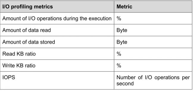
3.3 I/O operations

I/O operations are one of the kinds of operations that take more time to run. When applications run big amount of I/O operations the execution time is affected, slowing down the final solution and creating, normally, other performance issues like memory issues.

Understanding the IO profile or IO behaviour of your application is almost non-existent yet it is one of the most important things needed when designing a storage system. If we understand how our applications are performing IO then you can determine the performance requirements of your storage.

• How much capacity? • How much throughput? • How many IOPS?

(14)

Date: 29/03/2013 Page 13 / 50

• What is the latency to access the first element of a dataset? • How much time is spent performing IO?

I/O profiling metrics Metric

Amount of I/O operations during the execution %

Amount of data read Byte

Amount of data stored Byte

Read KB ratio %

Write KB ratio %

IOPS Number of I/O operations per

second Table 3 I/O Metrics

3.4 Network

Network is a basic brick on distributed systems as its name has implicit the use of a network connection in order to interact with parts of the system that are not running in the same server.

Monitoring the network usage of our application will allow us to realize the following actions:

• Develop of traffic profiles for specific network segments

• Diagnose bandwidth-capacity issues for links that do not meet user expectations

• Analyze possible capacity issues that contribute to performance delay

I/O profiling metrics Metric

Number of messages interchanged Packet sent/received per seconds

Bandwidth KB

(15)

Date: 29/03/2013 Page 14 / 50

Table 4 Network Metrics

3.5 Power and Energy

To improve the energy efficiency of high-performance systems and applications, it is critical to profile the power consumption of real systems and applications at fine granularity. Combined with time (application length), this profile is used to compute the total energy consumed by applications.

Power consumption, and hence power profiling, can be seen as a profile combination of the sections before. Multiple sub-systems of a computer consume power: CPU, memory hierarchy, network interfaces,... Usually all sub-systems are connected by a shared bus. During the lifetime of an application, as the bus is shared, there is a balance of usage between CPU, memory and I/O. Thus, as power consumption follows mainly usage, usually:

• CPU power decreases as memory power consumptions goes up

• CPU and memory power decrease with message communication among different nodes

• For most parallel codes, the average power consumption goes down as the number of nodes increase

• Communication distance and message size affects the power profile pattern.

In some cases those general remarks are not valid when there is communication and computation overlap for example.

4 How to measure

In this section we will present a set of tools used for monitoring and profiling applications. The tools presented here will cover different aspects and different places where to take the information from. We will see how to use the compilers, taking information from the source code, directly using specific hardware monitoring at the CPU, using the Operating System in order to measure the interactions with the OS and diving also into the virtualized paradigm gathering information from such systems. Please not that it is currently impossible to directly measure power, energy and heat produced by a single application. Indirect measurement tools are described in the deliverable D5.3 and more generally in the task T5.2. The measurement tools provided in this section are the one used to compute power at the application level. Otherwise, to obtain power it is necessary to use the dedicated watt-meter available on the CoolEmAll platform. Its usage is described in the deliverable D2.4.

(16)

Date: 29/03/2013 Page 15 / 50

4.1 Static program modification

This category of profiling tools tackles directly the source code on one hand when this is available and the binaries on the other hand. The idea behind this technique is to record desire events at run time.

When the source code is available, it is possible to set the compiler to instrument the source code, inserting tags that would leave execution trace for symbolic and syntactical information of the source code. When the source code is not available the information retrieved would not have similar accuracy as the one available with the source code, but with the following tools we can instrument almost every binary.

4.1.1 Gprof

Gprof1 is an open source call graph execution profiler that creates a call graph detailing which functions in a program call which other functions and records the amount of time spent in each. To use gprof we must compile our source code with support for this profiling application monitor. With this support, gprof will insert desired monitoring routines in the source code in order to gather information.

The accuracy of this information is higher if we compile the whole application with this support, meaning that if we use external libraries that are not compiled with gprof we won’t get any information from them.

Flat profile:

Each sample counts as 0.01 seconds.

% cumulative self self total time seconds seconds calls ms/call ms/call name 33.34 0.02 0.02 7208 0.00 0.00 open 16.67 0.03 0.01 244 0.04 0.12 offtime 16.67 0.04 0.01 8 1.25 1.25 memccpy 16.67 0.05 0.01 7 1.43 1.43 write 16.67 0.06 0.01 mcount 0.00 0.06 0.00 236 0.00 0.00 tzset 0.00 0.06 0.00 192 0.00 0.00 tolower 0.00 0.06 0.00 47 0.00 0.00 strlen 0.00 0.06 0.00 45 0.00 0.00 strchr 0.00 0.06 0.00 1 0.00 50.00 main 0.00 0.06 0.00 1 0.00 0.00 memcpy 0.00 0.06 0.00 1 0.00 10.11 print 0.00 0.06 0.00 1 0.00 0.00 profil 0.00 0.06 0.00 1 0.00 50.00 report

Table 5 Gprof flat profile report

1 _{http://www.gnu.org/software/binutils/}

(17)

Date: 29/03/2013 Page 16 / 50

4.1.2 ATOM

Analysis Tools with OM (ATOM)[36] is a framework to develop application monitoring routines written for the Alpha AXP processor which is similar to the Etch (described below) framework on x86. The framework provides with tools to the user for to specify instrumentation point and actions. Such instrumentation routines will work on the object files at compilation time.

Developers must tell atom where to insert the routines using a special programming language that later on will be used to break the source code in small procedures allowing the framework to time each fragment separately. The following example shows how to create a routine using atom:

Instrument(int iargc, char**iargv) { Proc* p; Block *b; Inst *inst; AddCallProto("OpenRecord()"); AddCallProto("CloseRecord()"); AddCallProto("Load( VALUE)"); for(p=GetFirstProc();p!=NULL;p=GetNextProc(p)){ for(b=GetFirstBlock(p);b!=NULL;b=GetNextBlock(b)){

for (inst = GetFirstInst(block); inst != NULL; inst = GetNextInst(inst)){ if(IsInstType(inst, InstTypeLoad){

AddCallInst(inst, InstBefore, "Load", EffAddrValue); } } } } AddCallProgram(ProgramBefore, "OpenRecord"); AddCallProgram(ProgramAfter, "CloseRecord"); } 4.1.3 Etch

Etch[37] is a similar framework as ATOM but created for X86 processors that would let us profile Windows applications. Despite of ATOM Etch works also on binary executable files, meaning that it is not needed to have the source code in order to generate a profile with Etch.

After an Etch profiling it is possible to ask Etch to modify the binary. This modification rearranges instructions in the binary file and increase a specific performance on one of the aspects of the application. The available operations of Etch are limited as the results of the modified binary must be the same as of the original.

4.1.4 Java profiling

Modern programing languages also provide with different frameworks that allow developers to perform profiling analysis of their applications. Nowadays these frameworks are also integrated in editors like eclipse or NetBeans2.

2 _{http://netbeans.org/}

(18)

Date: 29/03/2013 Page 17 / 50

The Eclipse Java Profiler3 is both a tool for profiling and an extensible framework. It consists of the Profiling and Logging Perspective and a number of views. It enables you to profile your applications, to work with profiling resources, to interact with the applications you are profiling, and to examine your applications for performance, memory usage and threading problems.

Java profiler allows you to profile aspects like: • Memory

• CPU • Thread

• Pattern extraction • Distributed monitoring

The java profiling tool integrated in eclipse provides a graphical user interface and specific views providing the developer to select the class or method to profile. The specific view will run the profiling test directly from the editor, showing after the execution a graphical report with the relevant information. The following figure shows a report run on a class, showing information about the timing needed to execute a certain task

3 _{http://www.eclipse.org/tptp/}

(19)

Date: 29/03/2013 Page 18 / 50

Figure 1 Java profiling tool report

4.2 Hardware counters

Hardware counters are monitoring tools for profiling applications that are inserted directly in the CPU, these tools provide a very fine grain information about the software execution. This type of application monitoring is very dependent of the architecture and manufacturer of the processor. Generally this information is retrieved in using the OS Kernel of tools for such porpoise.

The counters can generally be configured to gather information of different components of the CPU like the cache or the main memory. Running the application different times with a different monitor enabled would give us a perfect profile of the CPU consumption of our application

(20)

Date: 29/03/2013 Page 19 / 50

4.2.1 PAPI

Performance API (PAPI)4 is an application that implements access to most of the hardware performance counters available on modern processors. PAPI can be used as a simple application to extract general information from the processor counters or can be used as a programming framework to extract and manipulate metrics to obtain rich information. This API is an extraction layer for the specific API implemented on a specific architecture. This feature allows developers to program the same monitoring script for the software and run it on different platforms to find the best performance profile for their application.

PAPI currently supports the most common processors available in the market, in the following table we can find the supported processors in the last version of the API.

Operating System Processor Driver Notes

AIX 5.x IBM POWER5, POWER6 bos.pmapi xlc 6+

AIX 6.x IBM POWER7 bos.pmapi under

development Cray Linux

Environment 2.x, 3.x

Cray XT{3 - 6}, XE{5, 6} none

Compute Node Kernel

IBM Blue Gene P none

FreeBSD x86, x86_64 (Intel, AMD) HWPMC driver

Linux x86, x86_64 (Intel, AMD) PerfCtr 2.6.x kernel 2.6.x Linux x86, x86_64 (Intel, AMD) Perfmon2 kernel 2.6.30

and below Linux x86, x86_64 (Intel, AMD),

ARM, MIPS

perf_events kernel 2.6.32 and above Linux Intel Itanium II, Montecito,

Montvale

Perfmon2 Linux 2.6.30 and below

4 _{http://icl.cs.utk.edu/papi/}

(21)

Date: 29/03/2013 Page 20 / 50

Linux IBM POWER4, 5, 6, 7 PerfCtr 2.7.x

Linux IBM POWER4, 5, 6, 7 perf_events kernel 2.6.32 and above

Linux IBM PowerPC970,

970MP

PerfCtr 2.7.x

Solaris 8, 9 UltraSparc I, II & III none

Solaris 10 Niagara 2 none

Table 6 PAPI supported processors

The following output shows PAPI information of the available events occurring currently in the processor, providing valuable and specific information about the type of processor where the software is running:

4.3 Kernel Profiling

Kernel profiling is very useful to understand and tune the OS execution that would reflect on the execution of the software running at that time. This type of profiling is interesting as all the system calls will go through the OS Kernel to reach the hardware components. Understanding the kernel0s effect on hardware event such as cache misses or clock ticks consumed may be inadequate; a more comprehensive framework that captures the relevant state of the kernel’s data structure is important, and cannot be achieved using only hardware counters.

%> papi_avail

Available events and hardware information.

--- Vendor string and code : AuthenticAMD (2)

Model string and code : AMD K8 Revision C (15) CPU Revision : 2.000000

CPU Megahertz : 2592.695068 CPU's in this Node : 4

Nodes in this System : 1 Total CPU's : 4 Number Hardware Counters : 4 Max Multiplex Counters : 32

--- The following correspond to fields in the PAPI_event_info_t structure.

(22)

Date: 29/03/2013 Page 21 / 50

4.3.1 Oprofile

Oprofile5 is a system profiler of the Linux Kernel. Since the release of the 2.6 version of the Linux kenrel, Oprofile is natively supported as a module, being needed to compile the software as a separated module for previous releases. Oprofile provides information about the system calls to the OS and the routines associated. It makes use of the hardware counters explained above and internal information of the kernel. This last feature allows the profiler to obtain memory failure statistics or predict failures of the TLB (Translation Lookaside Buffer). As we are talking about a low level monitoring (remember that the kernel is the first software layer in the OS stack) the information obtained is close linked to the hardware. This can be an impediment when executing the application on different architectures as some of them provide with more information than others.

To use Oprofile we have to have activated this feature in the kernel, the module blelow is the one in charge of enable this feature:

[*] Profiling support (EXPERIMENTAL)

<M> Oprofile system profiling (EXPERIMENTAL)

The following example shows the profile information available after an execution of a single program including external libraries needed:

$ opreport --demangle=smart --symbols `which lyx` CPU: PIII, speed 863.195 MHz (estimated)

Counted CPU_CLK_UNHALTED events (clocks processor is not halted) with a unit mask of 0x00 (No unit mask) count 50000

vma samples % image name symbol name

081ec974 5016 3.1034 lyx _Rb_tree<unsigned short, pair<unsigned short const, int>, unsigned short const>::find(unsigned short const&)

00009f30 4154 2.5701 libpthread-0.10.so __pthread_alt_unlock

0810c4ec 3323 2.0559 lyx Paragraph::getFontSettings(BufferParams const&, int) const 081319d8 3220 1.9922 lyx LyXText::getFont(Buffer const*, Paragraph*, int) const 080e45d8 3011 1.8629 lyx LyXFont::realize(LyXFont const&)

0000a120 2853 1.7652 libpthread-0.10.so __pthread_alt_lock 080e3d78 2623 1.6229 lyx LyXFont::LyXFont()

00069a10 2467 1.5263 libstdc++.so.5.0.1 string::find(char const*, unsigned, unsigned) const 0006a430 2274 1.4069 libstdc++.so.5.0.1 string::compare(char const*) const

4201e850 2169 1.3420 libc-2.3.2.so __GI_setlocale 4207d870 1982 1.2263 libc-2.3.2.so memcpy

Table 7 Oprofile output report

(23)

Date: 29/03/2013 Page 22 / 50

4.3.2 DTrace

DTrace6 is another Kernel profiling tool as Oprofile, but in this case is specific for Solaris OS, developed by sun to profile and obtain a better performance of their Spark servers, DTrace is still in use nowadays as part of the OpenSolaris OS and it has been ported to support other OS like FreeBSD and Max OX.

DTrace can execute profiling at runtime, only executing monitoring tasks when the user starts a profiling job, this way DTrace will not generate unnecessary calls to the Kernel and processor counters to delay the execution of an application. Despite of Oprofile, DTrace allows developers or advance users, generally administrators, to choose which kernel modules (denominated providers) to monitor on each execution. Hence, the output report will be specific for a profile rather than giving a general output of the execution if this is not the purpose.

Dtraces executions are called proves and in order to improve performance and cut down on the amount of data that the system has to deal with, the proves can be associated with a predicate that lays out the conditions under which the probe will be fired.

The following example shows an output of DTrace cinnamon-freebsd# dtrace -s d.d

function | nanoseconds per second kernel`ipport_tick 19215 kernel`nd6_timer 21521 kernel`lance_watchdog 31848 kernel`kbdmux_kbd_intr_timo 34418 kernel`logtimeout 106167 kernel`pffasttimo 149003 kernel`scrn_timer 157988 kernel`tcp_isn_tick 161720 kernel`pfslowtimo 201723 kernel`dcons_timeout 309218 0xc42deeb0 443589 kernel`lim_cb 584293 kernel`atkbd_timeout 789599 0xc42d34f0 807851 kernel`sleepq_timeout 4198977

Table 8 DTrace output report

6 _{http://dtrace.org/}

(24)

Date: 29/03/2013 Page 23 / 50

4.4 Virtual Images

Virtualization is a common used technology that day by day is generating more expectation and business. With the popularity of cloud computing in almost all the aspects of the modern computing these systems have to be profiled to optimize the execution of the software installed in the virtual images.

While the software installed in the virtual image can be treated in the same way as if it was installed in the host, hence we can apply the techniques and tools described above.

4.4.1 XenoProf

This utility allows administrators and developers of virtual services to collect information from virtualized infrastructures running on XEN. XenoProf7

instruments the hypervisor and the gest OS to use the underlying hardware performance counters as if they were used by Oprofile. This feature limits the use of XenoProf to instrument only open source operating systems, as in the case of Oprofile, it is needed to modify the kernel of the instrumented systems.

The Xenoprof supports system-wide coordinated profiling in a Xen environment to obtain the distribution of hardware events such as clock cycles, instruction execution, TLB and cache misses, etc. Xenoprof allows profiling of concurrently executing virtual machines (which includes the operating system and applications running in each virtual machine) and the Xen VMM itself.

% D-TLB miss Function Module

9.48 e1000 intr network driver 7.69 e1000 clean rx irq network driver 5.81 alloc skb from cache XenoLinux

4.45 ip rcv XenoLinux

3.66 free block XenoLinux

3.49 kfree XenoLinux

3.32 tcp preque process XenoLinux 3.01 tcp rcv established XenoLinux

Table 9 TLB miss distribution in Xen Dom0

4.4.2 Virtualized performance counters

XenoProf, described on section 4.4.1, makes use of the OS kernel because of the paravirtualization executed on XEN. However, on pure virtualized systems this information cannot be used and hence, VMWare is working on another approach: Virtualize hardware performance counters.

7 _{http://xenoprof.sourceforge.net/}

(25)

Date: 29/03/2013 Page 24 / 50

Virtualization of hardware performance counters are not such a trivial work as the Virtual CPU (VCPU) does not use the Physical 100% CPU when executing instructions as some of them are caught for the hypervisor, resetting the counter to 0.

The result is to use a combination and synchronization of emulated and native performance counters, finding the following 3 approaches:

• one approach is to allow the counters to run during execution of the inner portions of the emulation code, and to pause the counters only on context switches away from the current VCPU

• Another approach pauses all counters at the boundary between hypervisor and hardware execution of guest code

• The last approach emulates the hardware counters to attempt to represent the microarchitecture's counts for a small subset of events

Finally the common approach used in VMWare makes the hypervisor to handle guest performance counters proxying the flow of information from the guest to the physical counter. This work of proxy the information allows the hypervisor to synchronize the counters when an interruption in the execution of a function is intercepted and resuming the counting at the same time as the execution resumes.

4.5 Parallel systems

This type of profiling presents extra challenges as in the case of the virtualization profiling. This is caused because the computational logic is distributed among different nodes. And monitored events raise on different levels.

4.5.1 ZM4/SIMPLE

This hybrid combination of hardware and software combined monitoring system uses event driven monitoring. By using this event driven monitoring, different nodes do not have to be simultaneously monitored, but when an event is raised this is caught.

ZM4 is the hardware component of the system, it consist of a control and evaluation computer (CEC) that control the actions of multiple monitor agents distributed among the cluster. The monitor agents are a set of nodes with special hardware integrated with the specific functionality of timestamping and recoding events in the distributed system. This hardware distributed monitored agent uses the Ethernet connection to send the information back to the central node, the CEC where the distributed application profile information is later sorted using a synchronized global system clock.

(26)

Date: 29/03/2013 Page 25 / 50

5 Application characterization

5.1 Behaviour characterization

Classification can be based on information provided by the tools and techniques described in the previous sections or based on the application behaviour. Classification will be used in order to tune systems parameters (network speed, processor frequency,...). Several applications impact the system in the same manner, depending only on their behaviour. Even if being more complex than simply asking the user the category of its application, in CoolEmAll behaviour detection is used: It reduces user burden: Indeed users don’t have to specify which type of application they run. It also remove the possibility to cheat the system (and the system administrator),

Without a-priori information (such as application name) it is necessary to obtain information on the application behaviour. Several possibilities are available: Process information (performance counters, system resources used), Subsystem information (network, disks) and Host information (power consumption).

We will see in the following that using all those information for one particular application allows for deriving in which category it fits. It enables also to understand in which phase this application is (computing, communicating, ...). Efforts to model applications power/energy consumption via performance monitoring counters have shown that performance monitoring counters relevant to power consumption estimation depend on the application itself. Thus performance counters relevant to power consumption estimation of a CPU intensive application may differ from those relevant to power consumption estimation of a memory intensive application.

As performance monitoring counters relevant to power consumption estimation depends on the computational state of the application, any change in the set of performance counters relevant to power consumption estimation of an application over a time period T reflects a change in the application computational state over the same time period T.

Figure 2 illustrates this change in application state. It shows how, by using performance counters, it is possible to detect two alternating phases.

The behaviour of an application will then be defined according to the consumption of resources it induces. This consumption will be monitored using real-time monitoring capabilities described in the previous section. Each second a vector of monitored data will define the behaviour of an application during this second. This vector will be called « Execution Vector ». As storing and aggregating all those vectors (one per second per application per host) would have to much impact on the infrastructure and on the applications, this vector is aggregated (averaged) for the duration of an application or a phase in order to obtain a « Signature vector ». This signature vector represents the resource consumption of the application or phase and can be used as input to simulation

(27)

Date: 29/03/2013 Page 26 / 50

or comparison between applications of phases.

Figure 2: Example of the monitoring of an application where two phases are alternating. The red line is an evaluation of the change in resource consumption between one second and the next. Peaks in the red line area good indicator of phase change.

Then, to evaluate if an application changed phase it is possible to evaluate the difference between consecutive EV (Execution Vector). If this difference goes over a threshold, it can be considered as a change of phase. Global behaviour is illustrated in figure 3.

5.2 Phase identification

If current signature vector is within a threshold distance of a past signature vectors, these two phases are considered as identical. Otherwise a new phase is added by adding the signature vector to the reference vector list.

This identification can only be done once the detection of a phase is finished. It can be useful to identify earlier a phase without waiting for its end. It is possible using partial recognition.

To improve reactivity partial recognition technique is used to identify phases before their completion. Once a phase is completed, its reference is stored along

(28)

Date: 29/03/2013 Page 27 / 50

with its length and its characteristics. Thus, an ongoing phase (a phase started but not yet completed) is recognized as an existing phase if the Manhattan distance (the Manhattan distance defines the degree of similarity between two execution vectors, one may chose another metric) between each execution vector of the already executed part and any reference vector is within the a given threshold defining the percentage of dissimilarity between them. We speak of an X% recognition threshold if the already executed part of the ongoing execution is equals to X% of the length of any existing stored phase.

5.3 DNA-like System Modelling

The application profiles repository contains description of applications required by simulations. In classical simulation, application are usually described by their submission time and length. In our context, it is insufficient to evaluate the power and thermal impact of the application.

Figure 3: Phase detection and identification with partial recognition

We will use the DNA-inspired[24] formalism to describe applications. The goal of this formalism is to obtain a profile of resource consumption of applications. Using these information of the resources consumed, simulation can evaluate the impact of this application on the system, using models[25] to translate these resources into power and energy. Then, it is possible to evaluate the thermal impact using energy dissipation models.

(29)

Date: 29/03/2013 Page 28 / 50

In this formalism, an application is considered to have phases. An application can start using disk, then do some communication and finally use disk again. This application is modelled as having three phases. The DNA-inspired approach assigns a letter (like AGTC for human DNA) to each phase. A letter describe the resource consumption of a phase as described bellow. If two phases have the same resource consumption profile, they will be assigned the same letter. The application description is then a chromosome, a sequence of such letters. A distributed application is described as a set of chromosome. An example is shown on figure 1, an application has two types of phases, repeted several times, which can be detected as the values of the hardware performance counters cache references, branch instructions and branch misses have different behaviours. In our formalism, this sequence would be encoded as

A{106}B{11}A{106}B{11}...A{106}B{11} for the chromosome part, as the first

phase lasts 106 seconds and the other phase lasts 11. It is associated with a profile of resource consumption for A and B.

A letter itself is modelled as a column vector of hardware monitoring counters including performance counters, system values, disk read/write and network bytes (respectively packets) sent/received counts to capture non memory- or CPU-intensive behaviour and length.

In the application profile repository, each application chromosomes will be stored along with the hardware description on which it has been obtained. A translation tool is used to translate letters from the original monitored hardware to the one aimed during the simulation. For instance, if the letter describes a full CPU application, the translation will use the ratio of frequencies between the original and the destination.

6 Application and phase classification

Certain applications share similar characteristics, making them comparable to each other. This is the same for phases. Two different applications can have a particular phase in common, like an I/O phase where results are saved for instance. In the following we will assimilate phases and applications and use only the term application. The question arises how to compare them and to differentiate their impact on the system from different point of view: Power, energy and heat.

(30)

Date: 29/03/2013 Page 29 / 50

Figure 4: Several Nas Parallel Benchmark. X axis is the mean power consumed, Y axis is the mean number of cache misses per second

To be precise, having more than simple load is necessary. For instance, in Figure 4, all the benchmarks have a 100% load. However their power profiles are different. In fact, even having the load profile and the memory access profile is in this case insufficient and would lead to 7% of error in the evaluation of power by an application: IS and FT have the same resource consumption profile for CPU and memory but have a power consumption that differs of 16W on the same hardware. IS and FT are two benchmarks of the Nas Parallel Benchark8 suite that have different patterns of access to the memory and network.

6.1 Methodology for classification of applications

The methodology of the application classification is the following. Initially different performance counters are monitored during application execution, such as cycles_persec, instructions_persec, minor.faults_persec. Their values are collected throughout application run. It is later necessary to remove correlated performance counters, as it is undesirable to have multiple variables carrying the

(31)

Date: 29/03/2013 Page 30 / 50

same information. An array with the values representing correlations between all performance counters is created. In case the correlation between two variables is higher or equal to 90%, the script needs to choose one to remove. To do that it calculates the correlation between these two performance counters and power usage. Variable with lower correlation is discarded.

After this phase the application is represented as a d-dimensional vector, each dimension being one performance counter. To create the groups of applications sharing similar characteristics, the hierarchical clustering with the Ward’s method is used, where the objective function is the error sum of squares. It minimizes the total within-cluster variance. At each step, the pair of clusters that leads to the minimum increase in total within-cluster variance after merging is selected. The result of this method is a dendrogram, a special tree structure that shows the relationships between clusters [27].

It is important to note that only applications utilizing the same number of cores and running on the same CPU frequency (it is best to use the highest value) should be used in the clustering method. This results from the fact that restricting application to a lower number of CPU cores or changing clock rate to a smaller value can significantly change application characteristic. As a result, the same program executed in different environments could be assigned to different clusters of applications.

To automate the process of group selection at runtime, a decision tree is created. It is a tree-shaped diagram that determines a course of action. Each branch of the decision tree represents a possible decision or occurrence. The tree structure shows how one choice leads to the next. The decision tree can be produced by multiple algorithms that identify various ways of splitting a data set into classes. Their representation of acquired knowledge in a tree form is intuitive and easy to understand by humans. What is more, the learning and classification steps of decision tree induction are simple and fast.

The algorithm for decision tree induction follows a greedy top-down approach, where the tree is constructed in a top-down recursive divide-and-conquer manner. It starts with a training set of tuples and their associated class labels. The training set is recursively partitioned into smaller subsets as the tree is being built. The attribute selection method specifies a heuristic procedure for selecting the attribute that ”best” discriminates the given tuples according to class. This procedure employs an attribute selection measure.

The tree starts as a single node, N, initially representing the complete set of training tuples and their associated class labels. If the tuples are all of the same class, the node N becomes a leaf and is labeled with that class. Otherwise, the attribute selection method is used to determine the splitting criterion. It specifies the attribute to test at node N by determining the ”best” way to separate or partition the tuples into individual classes. The splitting criterion is determined so that, ideally, the resulting partitions at each branch are as ”pure” as possible. A partition is ”pure” if all of the tuples in it belong to the same class.

(32)

Date: 29/03/2013 Page 31 / 50

Then the node N is labelled with the splitting criterion, which serves as a test at the node. A branch is grown from the node N for each of the outcomes of the splitting criterion. The tuples are partitioned accordingly. There are two possible scenarios – the splitting attribute may be discrete-valued or continuous-valued. In case of performance counters the latter situation always takes place, as they have numerical values. The test at node N has two possible outcomes, corresponding to the conditions A ≤ split_point and A > split_point, where split_point is the split-point returned by the attribute selection method.

The algorithm uses the same process recursively to form a decision tree for the tuples at each resulting partition. The recursive partitioning stops when all of the tuples belong to the same class, or there are no remaining attributes on which the tuples may be further partitioned, or there are no tuples for a given branch.

6.2 Experiments

6.2.1 Experimental setup

The above presented methodology was used to perform experiments. Three servers were used to validate the results:

• Sun Fire V20z with 4 x 2GB DDR RAM modules and 2 x dual-core AMD Opteron 275 “Italy” with 64KB L1 cache per core, 1MB L2 cache per core, 68W TDP, 1GHz HyperTransport bus and four P-States: 1.0GHz, 1.8GHz, 2.0GHz and 2.2GHz,

• Actina Solar 410 S2 with 4x 2GB DDR2 PC2-5300 RAM ECC-enabled RAM modules and 2x quad-core Intel Xeon E5345 „Clovertown” with 16KB L1 per core, 8MB shared L2 cache, 80W TDP, 1333MT/s FSB and two P-States: 2.0GHz and 2.33GHz,

• Actina Solar 212 X2 with 4x 2GB DDR2 PC2-5300 RAM ECC-enabled RAM modules and 2x 2 core Intel Xeon 5160 „Woodcrest” with 64KB Level 1 cache per core, 4MB shared Level 2 (L2) cache, 80W Thermal Design Power (TDP), 1333MT/s Front-side Bus (FSB) and four P-States: 2.0GHz, 2.33GHz, 2.66GHz and 3.00GHz.

The applications executed in the experiments were the following:

• Abinit – it is a software for materials science, computing electronic density and derived properties of materials ranging from molecules to surfaces to solids [28]. It can be deployed as a parallel workload using MPI. In the given tests, Abinit was used to calculate one of the example inputs shipped with the source package,

• Cavity – the lid-driven cavity is a CFD problem for testing new CFD algorithms and has long been used as a test or validation case for new codes or new solution methods [29, 30]. In the given tests the problem

(33)

Date: 29/03/2013 Page 32 / 50

was solved with the Lattice Boltzmann methods (using Palabos, an open-source CFD library),

• C-Ray – it is a simple ray-tracing benchmark, usually involving only a small amount of data [31]. This software measures floating point CPU performance, often even not accessing main RAM. The test is configured with a significantly big scene, requiring about 60s of computation but the resulting image is written to /dev/null to avoid the disk overhead,

• CPU Burn – it is a stability testing tool for overclockers. The program heats up the CPU to the maximum possible operating temperature that is achievable by using ordinary software. In these tests burnK7 is used on the AMD machine and burnMMX on the Intel CPUs [32],

• HMMER – it is a software for sequence analysis. Its general usage is to identify homologous protein or nucleotide sequences. This type of problem was chosen because it requires a relatively big input size (hundreds of MB) and requires specific types of operations related to sequences [33],

• NAMD – it is a molecular dynamics simulation package written using the Charm++ parallel programming model, noted for its parallel efficiency and often used to simulate large systems of atoms. The software is mainly written in C++ and can be deployed as an MPI workload. One of the examples shipped with the source package was used as input [34],

• MEncoder – it is a command line video decoding, encoding and filtering tool, able to convert multiple formats into a variety of compressed and uncompressed formats using different codecs [35]. The test consists of encoding a raw 1080p video stream into H.264. The content is a 20s part of Big Buck Bunny video, a free content video licensed under the Creative-Commons license.

In the experiments, the Perf Tool [26] was used. It makes access to the performance counters very easy, as it presents a simple command line interface by abstracting away CPU hardware differences in Linux performance measurements. It is based on the perf_events interface, available since Linux Kernel 2.6.31. The Perf tool offers a rich set of commands to collect and analyze performance and trace data.

6.2.2 Results

Using hierarchical clustering on AMD Opteron 275 to group applications results in a dendrogram, which is presented in Figure 5. Three clusters can be easily distinguished, represented in this Figure as three red boxes. The distances between them are quite high, as opposed to the distances between applications inside clusters, which suggests that the groups were selected properly. It is also very conforming that no instance of any application (in other words – no

(34)

Date: 29/03/2013 Page 33 / 50

application execution) was assigned to more than one group. It confirms the suggestion that the groups have their own characteristics, not shared with other clusters.

The extracted groups were the following: • Ist group: abinit, burn and namd, • IInd group: cavity,

• IIIrd group: c-ray, hmmer, mencoder.

Figure 5 Arrangement of clusters of applications on AMD Opteron 275

Moreover, it is necessary to distinguish fourth group – idle. It contains the periods without any application execution.

The decision tree created for these four groups is presented in Figure 6. Two paths in the tree lead to class I, another two to class III and there are three other paths, one for each of the other classes. Only three variables were used to

(35)

Date: 29/03/2013 Page 34 / 50

differentiate between classes of applications: perf.instructions_persec, perf.cache.misses_persec and perf.DRAM.access.1_persec. Those values represent respectively their mean number of instruction per second, mean cache misses per seconds and mean DRAM access per second. It is important to note that the tree correctly classifies all of the training data points.

Figure 6 Classification Tree for AMD Opteron 275

The accuracy of the tree was examined by another software. All of the applications in the tree were executed by this program, at the same time the values of selected performance counters were compared to the ones appearing in the tree and the appropriate model was selected. The class resulting from the use of the tree was compared to the actual class of currently running application. In turned out that the tree correctly classified 95.79% of cases. Moments of misclassification appeared either at the beginning or end of application run, where the values of performance counters were not stabilized.

Similar experiments were performed for processor Intel Xeon E5345. Just like in the previous CPU, the hierarchical clustering was used to create clusters of applications. Because the characteristics of application changes when running on

(36)

Date: 29/03/2013 Page 35 / 50

different number of cores or CPU frequency, the highest frequency and number of cores (eight in this case) were used to execute the programs. The resulting dendrogram is presented in Figure 7.

Figure 7 Arrangement of clusters of applications on Intel Xeon E5345

The cut-off value of 15 was selected, creating three clusters of applications – the same as in case of AMD processor.

Similarly, to make it possible to choose an appropriate model at runtime, a decision tree was created for this processor. It is presented in Figure 8. As it turned out, only two variables were used to create the tree – perf.instructions_persec and perf.LLC.loads_persec. The tree is very simple, yet accurate – just as in the previous experiments, every application was correctly classified.

The experiments proved the tree to be very accurate – it correctly chose the correct group for 95-97% of the time. The incorrect choice of the model usually

(37)

Date: 29/03/2013 Page 36 / 50

took place during application launch or shutdown.

Figure 8 Classification tree for Intel Xeon E5345

The last set of experiments was performed on Intel Xeon 5160. The methodology of work was the same. The hierarchical clustering created dendrogram presented in Figure 8. Again, the same classes of applications were distinguished, as in the case of previous processors:

• Ist group: abinit, burn and namd, • IInd group: cavity,

• IIIrd group: c-ray, hmmer, mencoder.

Idle periods should be treated as an additional class.

The classification tree created for Intel Xeon 5160 is presented in Figure 9. It it very simple, created with just three variables – perf.instructions_persec, perf.bus.trans.mem_persec and temp.cpu_avg.

(38)

Date: 29/03/2013 Page 37 / 50

Figure 9 Classification tree for Intel Xeon 5160

The tree was converted to a set of rules and in every second the model selected by the software assessing the tree accuracy was compared to the model appropriate for currently running application. As it turns out, the accuracy of the tree is 91,67%. Misclassification appeared mostly in two cases: when the application was started or when it finished calculations. In the first case wrong class was usually selected for about 1-2 seconds, the time needed for the performance counters to show stabilized values. However, when the application finished execution, wrong model (usually mencoder, c-ray hmmer instead of idle) was sometimes chosen for up to 1 minute. The reason behind this is the temperature variable. An analysis of the tree leads to the conclusion that idle class should be chosen only when the temperature reaches a value lower than 44.63 degrees Celsius. It always takes some time (between 5-60 seconds, depending on the starting temperature) for the processor to cool down.