HAL Id: hal-01914507
https://hal.archives-ouvertes.fr/hal-01914507
Submitted on 13 Nov 2020
HAL is a multi-disciplinary open access
archive for the deposit and dissemination of
sci-entific research documents, whether they are
pub-lished or not. The documents may come from
teaching and research institutions in France or
abroad, or from public or private research centers.
L’archive ouverte pluridisciplinaire HAL, est
destinée au dépôt et à la diffusion de documents
scientifiques de niveau recherche, publiés ou non,
émanant des établissements d’enseignement et de
recherche français ou étrangers, des laboratoires
publics ou privés.
Dense-gas tracers and carbon isotopes in five 2.5 < z <
4 lensed dusty star-forming galaxies from the SPT SMG
sample
M. Béthermin, T.R. Greve, C. de Breuck, J.D. Vieira, M. Aravena, S.C.
Chapman, Chian-Chou Chen, C. Dong, C.C. Hayward, Y. Hezaveh, et al.
To cite this version:
M. Béthermin, T.R. Greve, C. de Breuck, J.D. Vieira, M. Aravena, et al.. Dense-gas tracers and
carbon isotopes in five 2.5 < z < 4 lensed dusty star-forming galaxies from the SPT SMG sample.
Astron.Astrophys., 2018, 620, pp.A115. �10.1051/0004-6361/201833081�. �hal-01914507�
https://doi.org/10.1051/0004-6361/201833081 c ESO 2018
Astronomy
&
Astrophysics
Dense-gas tracers and carbon isotopes in five 2.5
<
z
<
4 lensed
dusty star-forming galaxies from the SPT SMG sample
M. Béthermin
1, T. R. Greve
2, C. De Breuck
3, J. D. Vieira
4, M. Aravena
5, S. C. Chapman
6, Chian-Chou Chen
3,
C. Dong
7, C. C. Hayward
8, Y. Hezaveh
9, D. P. Marrone
10, D. Narayanan
7,11,12, K. A. Phadke
4, C. A. Reuter
4,
J. S. Spilker
13, A. A. Stark
14, M. L. Strandet
15, and A. Weiß
151 Aix-Marseille Univ., CNRS, CNES, LAM, Marseille, France
e-mail: [email protected]
2 Department of Physics and Astronomy, University College London, Gower Street, London WC1E 6BT, UK 3 European Southern Observatory, Karl Schwarzschild Straße 2, 85748 Garching, Germany
4 Department of Astronomy and Department of Physics, University of Illinois, 1002 West Green St., Urbana, IL 61801, USA 5 Núcleo de Astronomía, Facultad de Ingeniería y Ciencias, Universidad Diego Portales, Av. Ejército 441, Santiago, Chile 6 Dalhousie University, Halifax, Nova Scotia, Canada
7 Department of Astronomy, University of Florida, Gainesville, FL 32611, USA
8 Center for Computational Astrophysics, Flatiron Institute, 162 Fifth Avenue, New York, NY 10010, USA 9 Kavli Institute for Particle Astrophysics and Cosmology, Stanford University, Stanford, CA 94305, USA 10 Steward Observatory, University of Arizona, 933 North Cherry Avenue, Tucson, AZ 85721, USA
11 University of Florida Informatics Institute, 432 Newell Drive, CISE Bldg E251, Gainesville, FL 32611, USA 12 Cosmic Dawn Centre (DAWN), University of Copenhagen, Julian Maries vej 30, 2100 Copenhagen, Denmark 13 Department of Astronomy, University of Texas at Austin, 2515 Speedway Stop C1400, Austin, TX 78712, USA 14 Harvard-Smithsonian Center for Astrophysics, 60 Garden Street, Cambridge, MA 02138, USA
15 Max-Planck-Institut für Radioastronomie, Auf dem Hügel 69, 53121 Bonn, Germany
Received 23 March 2018/ Accepted 9 October 2018
ABSTRACT
The origin of the high star formation rates (SFR) observed in high-redshift dusty star-forming galaxies is still unknown. Large fractions of dense molecular gas might provide part of the explanation, but there are few observational constraints on the amount of dense gas in high-redshift systems dominated by star formation. In this paper, we present the results of our Atacama large millimeter array (ALMA) program targeting dense-gas tracers (HCN(5-4), HCO+(5-4), and HNC(5-4)) in five strongly lensed galaxies from the South Pole Telescope (SPT) submillimeter galaxy sample. We detected two of these lines (S /N > 5) in SPT-125-47 at z= 2.51 and tentatively detected all three (S /N ∼ 3) in SPT0551-50 at z= 3.16. Since a significant fraction of our target lines is not detected, we developed a statistical method to derive unbiased mean properties of our sample taking into account both detections and non-detections. On average, the HCN(5-4) and HCO+(5-4) luminosities of our sources are a factor of ∼1.7 fainter than expected, based on the local L0
HCN(5-4)−LIRrelation, but this offset corresponds to only ∼2σ if we consider sample variance. We find that both the HCO+/HCN and
HNC/HCN flux ratios are compatible with unity. The first ratio is expected for photo-dominated regions (PDRs) while the second is consistent with PDRs or X-ray dominated regions (XDRs) and/or mid-infrared (IR) pumping of HNC. Our sources are at the high end of the local relation between the star formation efficiency, determined using the LIR/[CI] and LIR/CO ratios, and the dense-gas
fraction, estimated using the HCN/[CI] and HCN/CO ratios. Finally, in SPT0125-47, which has the highest signal-to-noise ratio, we found that the velocity profiles of the lines tracing dense (HCN, HCO+) and lower-density (CO, [CI]) molecular gas are similar. In addition to these lines, we obtained one robust and one tentative detection of13CO(4-3) and found an average I
12CO(4-3)/I13CO(4-3)flux
ratio of 26.1+4.5−3.5, indicating a young but not pristine interstellar medium. We argue that the combination of large and slightly enriched gas reservoirs and high dense-gas fractions could explain the prodigious star formation in these systems.
Key words. galaxies: ISM – galaxies: star formation – galaxies: high-redshift – galaxies: starburst – submillimeter: galaxies
1. Introduction
Traditionally, the molecular gas in high-redshift galaxies has been probed by observations of the rotational lines of CO (e.g., Solomon & Vanden Bout 2005). Systematic CO line surveys have shown an increasing molecular gas fraction with redshift (e.g., Tacconi et al. 2010, 2013; Saintonge et al. 2013; Carilli & Walter 2013; Dessauges-Zavadsky et al. 2015;
Aravena et al. 2016; Keating et al. 2016). Other methods based on the galaxy dust content found similar results (Magdis et al. 2012;Scoville et al. 2014,2016;Béthermin et al.
2015;Schinnerer et al. 2016). These analyses suggest that high star formation activity in massive galaxies observed at high redshift is related to their larger gas content. Furthermore, an increase in the star formation efficiency, that is, the star for-mation rate (SFR) relative to the total gas mass (as traced by CO or dust), seems necessary to account for the prodigious star formation in the most extreme systems (e.g., Engel et al. 2010;Genzel et al. 2010;Daddi et al. 2010;Magdis et al. 2011;
Tan et al. 2014;Hodge et al. 2015;Silverman et al. 2015). In contrast, we have much less information about the amount of dense, actively star-forming gas in high-redshift galaxies. The
Open Access article,published by EDP Sciences, under the terms of the Creative Commons Attribution License (http://creativecommons.org/licenses/by/4.0),
dense gas is usually traced using the rotational lines of high-dipole molecules such as HCN, which have H2critical densities
&104cm−3(Shirley 2015). WhileKauffmann et al.(2017) argue
that in some Galactic clouds the HCN(1-0) line traces gas den-sities similar to those traced by high-J CO lines (103cm−3), the
higher J transitions of HCN are still considered to be our best indicators of dense gas in galaxies.
As gas in the interstellar medium collapses to form stars, it passes though the density regime where the hydrogen is pre-dominantly molecular and is dense enough to excite rotational transitions of HCN and HCO+into emission (Larson 1994). For stars to form, the density must be sufficiently high in the star-forming cloud cores that self-gravity dominates over tidal shear. For much of the volume of a typical galaxy, the threshold density for collapse in spite of tidal shear and the threshold density for excitation of high dipole moment molecules into emission are approximately the same (Stark et al. 1989). The luminosity of the HCN line is then a good measure of the SFR. In the central kiloparsec of large galaxies, however, the density of the inter-stellar medium may be high enough to excite HCN but not high enough to resist the very much higher tidal shear in those regions of high differential rotation; the HCN line may then have a large beam-filling factor and be bright in emission from an extended, non-cloudy molecular gas, even though no star formation can take place.
In the local Universe,Gao & Solomon(2004) found that in log-log space, the HCN(1-0) luminosity is linearly proportional to SFR, as gauged by the total infrared luminosity (LIR), with
a small scatter over 2.5 decades in luminosity. The interpreta-tion of this result is that the SFR in galaxies is primarily con-trolled by the dense gas fraction. Linear luminosity relations have been found using CO(3-2), HCO+(1-0), HCO+(3-2), HCO+ (5-4), HCN(4-3), CS(5-4), CS(7-6), and formaldehyde dense observations of a subset of the same galaxies (Yao et al. 2003;
Narayanan et al. 2005;Graciá-Carpio et al. 2006;Mangum et al. 2008, 2013; Iono et al. 2009; Juneau et al. 2009; Wang et al. 2011;Zhang et al. 2014).
Observations of Milky Way clumps in HCN(1-0), as well as in a variety of other dense gas tracers, byWu et al.(2005,2010) found a roughly linear relation between the SFR and the dense-gas mass (Mdense) consistent with the galaxy-integrated
measure-ments. They arrive at the same interpretation asGao & Solomon
(2004), namely that the SFR of a galaxy scales linearly with the number of dense-gas “units” in a galaxy, with the dense-gas star formation efficiency being constant. Similarly, observations toward high visual extinction lines of sight byLada et al.(2010,
2012) andHeiderman et al.(2010) support this interpretation. In contrast,Bigiel et al.(2016) showed that the increase in dense-gas fraction towards the center of M 51 leads to a decrease in the dense-gas star formation efficiency (∝LIR/L0HCN), since there
will be fewer overdense regions able to gravitationally collapse if the average density is higher.
This interpretation, however, as well as the claimed lin-earity of the SFR-dense gas relation is debated in the lit-erature. For example, Bussmann et al. (2008) observe sub-linear IR-HCN(3-2) luminosity relations for nearby galaxies, while García-Burillo et al.(2012) found a slightly super-linear IR-HCN(1-0) luminosity relation. Both of these sets of observa-tions can be reconciled with simulaobserva-tions (e.g.,Narayanan et al. 2008b,2011). Similarly, star formation models suggest that the SFR-dense gas relationship is primarily set by the gas den-sity probability distribution function (PDF) in galaxies. As a result, a range of SFR-dense gas mass slopes may be expected, depending on the effective density of the tracer and the exact
form of the gas density PDF (e.g.,Krumholz & Thompson 2007;
Narayanan et al. 2008b; Hopkins et al. 2013; Popping et al. 2014; Onus et al. 2018). In a high-pressure turbulent interstel-lar medium (ISM), the average gas density is expected to be higher at all physical scales with a larger fraction of the total gas mass residing at higher densities (>104cm−3). This type of high-pressure turbulent ISM is more likely to occur in vigorously star-forming regions than in more quiescent ISM conditions (Papadopoulos 2010). This is supported by many numerical sim-ulations, which tend to predict a dramatic increase in the dense-gas fraction during major mergers causing a short (∼100 Myr) boost of the star formation efficiency (e.g.,Renaud et al. 2014). However, a recent study by Fensch et al. (2017) suggests that this phenomenon could not be efficient in mergers of two gas-rich galaxies at high redshift. Observational constraints are thus essential to test this result. HCN, HCO+, and CS studies of local (ultra-)luminous infrared galaxies (ULIRGS) have found high gas fractions (e.g.,Gao & Solomon 2004; García-Burillo et al. 2012; Zhang et al. 2014) – but so far this has not been firmly established at high redshift.
The detections of dense-gas tracers such as HCN and HCO+ remain scarce at high redshift due to the faintness of these lines (typically more than 10× fainter than CO). In fact, all such detec-tions to date were obtained with the assistance of gravitational lensing. Early efforts by, for example, Greve et al.(2006) and
Gao et al.(2007) to detect HCN(1-0) in high-z starburst galax-ies resulted only in upper limits. Most of the firm detections were obtained for quasars: for example, HCN(1-0) in the Clover-leaf at z= 2.6 by Solomon et al. (2003), IRAS F10214+4724 at z= 2.3 by Vanden Bout et al. (2004), and J1409+5628 at z= 2.6 byCarilli et al.(2005) and HCN(5-4) and HCN(6-5) in APM08279+5255 at z = 3.9 (Barvainis et al. 1997; Wagg et al. 2005;Weiß et al. 2007;Riechers et al. 2010). There are even fewer published detections of star-formation-dominated objects. The HCN(3-2) line was detected in SMMJ1213511-0102 at z= 2.3 by
Danielson et al.(2011) and recentlyOteo et al.(2017) reported two new detections of HCN(3-2) and HCO+(3-2) in SDP.9 and SDP.11 at z= 1.6 and z = 1.8, respectively (they also detected the 1-0 transition of these two molecules in SDP.9). So far, no detec-tion at z > 2.5 has been reported in systems dominated by star for-mation. However,Spilker et al.(2014) stacked all the cycle-0 Ata-cama large millimeter array (ALMA) spectral scans of the South Pole telescope submillimeter galaxy sample (SPT SMG, z∼3.9) and detected HCN(4-3), HCO+(4-3), and HCO+(6-5).
In this paper, we present deep ALMA observations of HCN(5-4) in a sample of five lensed dusty star-forming galax-ies (DSFGs) between z = 2.5 and z = 4 from the South Pole Telescope (SPT) sample (Vieira et al. 2010, 2013). We chose to target HCN(5-4), since the HNC(4-3) line is not observable beyond z = 3.2 and we want to observe the same transition in all the sources of our sample. The transition has a typical effec-tive excitation density of ∼106cm−3(Shirley 2015and is
there-fore a bone fide tracer of the densest molecular gas in galaxies. In addition to HCN(5-4), and since they can be observed at the same time, our observations also targeted the HCO+(5-4) and HNC(5-4) lines, which are dense-gas tracers in their own right. However, these two lines are harder to interpret because of their more complex chemistry. HCO+, being an ion, is dependent on the ionization of the dense molecular clouds and is thus a less direct tracer of these high densities (Papadopoulos 2007). The line ratio between HCN and HNC is dependent on the physical conditions and varies from ∼1 in dense dark clouds (Hirota et al. 1998) to ∼10−2in hot and dense regions of star formation like Orion (Schilke et al. 1992). In addition to the above lines, we
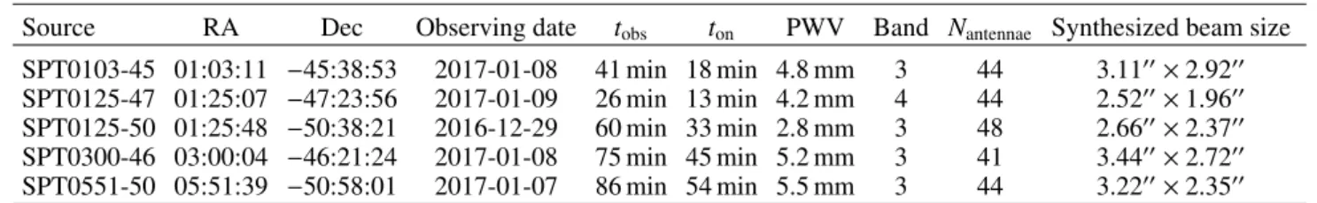
Table 1. Summary of the characteristics of our observations.
Source RA Dec Observing date tobs ton PWV Band Nantennae Synthesized beam size
SPT0103-45 01:03:11 −45:38:53 2017-01-08 41 min 18 min 4.8 mm 3 44 3.1100× 2.9200
SPT0125-47 01:25:07 −47:23:56 2017-01-09 26 min 13 min 4.2 mm 4 44 2.5200× 1.9600
SPT0125-50 01:25:48 −50:38:21 2016-12-29 60 min 33 min 2.8 mm 3 48 2.6600× 2.3700
SPT0300-46 03:00:04 −46:21:24 2017-01-08 75 min 45 min 5.2 mm 3 41 3.4400× 2.7200
SPT0551-50 05:51:39 −50:58:01 2017-01-07 86 min 54 min 5.5 mm 3 44 3.2200× 2.3500
Notes. Each source was observed in a separate ALMA scheduling block (SB). Two similar SBs were used for SPT0551-50, which required a longer integration. The total observing time and the time on source are tobsand ton, respectively. PWV is the average precipitable water vapor level
during our observations. The beam size in the table was derived using a natural weighting.
were able to simultaneously target the J = 4 − 3 transition of the 13CO isotopologue in four of our sources.13C is a
sec-ondary nucleus, which is not produced from fusion of hydrogen or helium in massive short-lived stars. Thus, detecting this line is a clue of previous star formation episodes in these galaxies (Hughes et al. 2008;Henkel et al. 2010).
In Sect.2we present our observations and our data reduc-tion and line extracreduc-tion methods. We then discuss the proper-ties of dense-gas tracers in Sect. 3. In Sect. 4, we compare the properties of dense and lower density molecular gas trac-ers (CO, [CI]). Finally, we present and interpret our measure-ments of the CO isotopes in Sect. 5. In this paper, we assume a Planck Collaboration XIII(2016) cosmology and a Chabrier
(2003) initial mass function (IMF).
2. Data
2.1. Observations
This paper is based on ALMA cycle-4 observations (2016.1.00065.S, PI: Béthermin) of five DSFGs from the SPT sample (Vieira et al. 2013;Weiß et al. 2013;Strandet et al. 2016), which were selected for having bright apparent infrared luminosities (LIR≥ 5 × 10¹³L ) and high-quality ancillary data.
ALMA bands 3 and, when needed, 4 were tuned to the redshifted frequencies of the HCN(5-4) transition. When possible, spare spectral windows of the correlator were placed such as to cover
13CO(4-3), HCO+(5-4), HNC(5-4), and [CI](1-0) (this latest
line is only observable in SPT0125-47). Each spectral window covers 1.875 GHz and contains 240 channels (coarsest frequency domain mode resolution with an online spectral averaging by a factor of 16). The previously mentioned lines are covered by two contiguous spectral windows in one of the side bands.
The sensitivities of the observations were determined to reach 5σ (10σ for SPT0125-47) using the L0HCN–LIR of
Zhang et al.(2014). Since our sources are gravitationally lensed and have an extension of ∼1 arcsec (Spilker et al. 2016), we requested the most compact configuration of the array to avoid spreading the flux of our sources over several synthesized beams and thus maximizing our chances to detect the integrated emis-sion of our objects. The characteristics of our survey are summa-rized in Table1. The observations were performed on December 29th, 2016 for SPT0125-47 and between January 7th, 2017 and January 9th, 2017 for the other sources. During our observations, the precipitable water vapor level (PWV) was between 2.8 and 5.5 mm.
2.2. Data reduction and extraction of the spectra
We analyzed our data with the CASA software (McMullin et al. 2007). They were initially calibrated by the standard ALMA
pipeline at the observatory. In addition, we manually flagged some antennae and spectral windows with poor bandpass, phase, or amplitude calibration. In particular, the antenna DA48 had y and z position offsets larger than 2 cm in all the January 2017 observations and its data were flagged systematically. The over-all quality of the rest of the data is very good.
The data were imaged using the CLEAN algorithm, and a natural weighting scheme was chosen to maximize the point-source sensitivity. We used cleaning thresholds corresponding to 3σ in a given channel using the map standard deviation around our source to estimate the noise. Since our lines are very broad and the signal-to-noise ratio (S/N) is low, the channels were again rebinned at the imaging stage. Because SPT0125-47 has several 5σ detections, we only needed a rebinning by a factor of four. Similarly, since SPT0300-46 and SPT0551-50 have at least one line above 3σ, we used a factor of six. For the remaining sources, we set the rebinning factor to eight.
We decided not to subtract the continuum directly in the uv plane. Instead, the continuum was subtracted later at the line extraction stage (see Sect.2.3). This choice was motivated by the presence of numerous broad lines in the two contiguous spectral windows of interest. The only good area of the spec-trum without line contamination is between the HCO+and the HNC line, but is too narrow to accurately constrain the slope of the continuum (see discussion in AppendixB). The imaging of the other side band, which is free of detected lines except for SPT0125-47, showed that, at the depth of our observations, the continuum varies significantly over 2 × 1.875 GHz. It is thus nec-essary to use a first-order subtraction of the continuum.
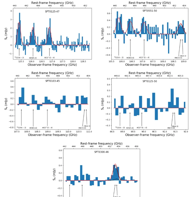
Before extracting the spectra, we checked that our sources are not significantly extended. We produced high S/N images by combining all the channels of the four spectral windows (mode multi-frequency synthesis). We fitted a two-dimensional Gaus-sian model and found the width of the GausGaus-sian to be consistent with that of the synthesized beam. Since the continuum emission of our sources is compatible with a point source at our ALMA res-olution, we thus extracted their spectrum from the ALMA cube at the centroid of this Gaussian model. Using this method, we implicitly assume that the size of the regions emitting the dense-gas lines is not much more extended than the continuum. The extracted spectrum corresponds to the two contiguous spectral windows in the side band of HCN(5-4) and is presented in Fig.1. 2.3. Line extraction
We extracted the lines by fitting the following model to the whole spectra. We assumed that the line profiles are Gaussian. We set a positivity prior on the line fluxes and allowed the full width at half maximum (FWHM) to vary between 200 and 1000 km s−1, which is typical for these types of sources (e.g.,Aravena et al. 2016).
Fig. 1.Continuum-subtracted spectra of our five sources (blue filled histograms). Two spectral windows were combined to produce them. The best fit of the baseline is subtracted from the data. The red solid line is our best-fit model and the black dashed line is the best-fit decomposition of the blend between HNC(5-4) and CN(4-3). Only lines with S /N > 3 are shown. The S/N of the blend between HNC(5-4) and CN(4-3) in SPT0551-50 only has an S/N of 2.6 using our deblending method, which could be underestimated. However, its S/N determined in AppendixB using the moment-zero map is 3.3. We thus included the line in the plot. The three bottom panels show sources with a low S/N. Their spectra were rebinned by a factor of two in the figure to allow a better visualization of the faint lines.
We allowed a velocity offset up to 200 km s−1 compared with
the expected center of the line based on the systemic red-shift estimated from the band-3 spectral scan of CO. Finally, we assumed a first-order baseline for the continuum emission of the sources. All the lines (13CO(4-3), HCN(5-4), HCO+
(5-4), HNC(5-4), and CN(4-3)) and the continuum baseline are
fitted simultaneously. This allows us to estimate the degenera-cies between the baseline parameters and the line properties. In AppendixB, we explain why this method rather than the classi-cal extraction in moment-zero maps was preferred.
We checked a posteriori from the residuals that these are fair assumptions. We found no significant feature in the
residual spectra. We computed the Pearson correlation coe ffi-cient between two neighboring channels and found that the cor-relation is lower than 0.2 for all our five residual spectra. Conse-quently, we can use these residuals to estimate the uncertainties on the line properties derived with our fit using a bootstrapping method. We thus took our best-fit model and added the residu-als after randomly reshuffling the channels. Then, we refitted the result and saved the obtained best-fit parameters. We repeated this 10 000 times. The error bars on the parameters are derived by computing the standard deviation of all these realizations. By construction, this method takes into account the degenera-cies between parameters, and in particular between the base-line determination and the base-line fluxes. We estimated the S/N by dividing the best-fit peak flux density by its uncertainty. Because of the combined uncertainties on the peak flux density and the width, the relative uncertainty on the line flux is slightly higher than on the peak.
Only SPT0125-47 and SPT0551-50 have sufficiently bright lines to fit them directly with reasonable constraints on the FWHM and the velocity offset for each line. For the other sources, even if there is systematically a positive signal at the position of the lines, the S/N is often lower than 3 and the width and velocity of the lines cannot be constrained. We thus assume in our fit that these two properties are similar for all the lines. The low-frequency wing of the SPT0125-4713CO(4-3) line is
not perfectly fitted, when the width and the velocity offset of each line are independent parameters. The FWHM is smaller than for other lines: 252 ± 45 versus 475 ± 128 and 496 ± 119 for HCN(5-4) and HCO+(5-4), respectively. However, this nar-rower profile is unlikely to be real (see Sect.5.2) and might be caused by the noise. To determine the best fit of13CO(4-3), we thus performed another fit assuming that the three lines have the same width and velocity offset. The flux is then slightly higher but consistent at 1σ with the previous value: 1.15 ± 0.22 versus 0.92 ± 0.15 Jy km s−1.
The results of our line extraction are summarized in Table2
and the best fit is shown in Fig.1(red solid line). When a line is not detected at ≥3σ, we derived a 3σ upper limit by sum-ming the best-fit flux measured in the spectrum and three times the standard deviation of the flux in our multiple bootstrap real-izations. Adding the signal present in the spectrum is crucial to obtain a reliable upper limit and is often forgotten in the litera-ture. Otherwise, a source detected with an S /N of 2.9999 would have an ∼50% probability of having a flux above the incorrectly computed 3σ upper limit.
When HNC(5-4) and CN(4-3) are both present in the spec-tra, a special method is used to extract them, since they are severely blended. The deblending of these two lines is discussed in Sect.2.6.
2.4. Detected lines
We detected three >5σ lines in SPT0125-47. 13CO(4-3), HCN(5-4), and HCO+(5-4) are detected at 7.2, 5.3, and 5.6σ, respectively. In SPT0551-50, there are ∼3σ peaks at the posi-tion of the four targeted lines (3.4, 3.0, 3.1, and 2.6σ for13CO
(4-3), HCN(5-4), HCO+(5-4), and HNC(5-4), respectively). For the other three sources, only the blend HNC(5-4) and CN(4-3) in SPT0300-46 has an S /N larger than 3. However, these other data are very useful as lower or upper limits and allow us to derive unbiased mean properties for our sample using the method pre-sented in Sects.2.5and2.6.
Previously, HCN(5-4), HCO+(5-4), and HNC(5-4) have been detected at high redshift only in quasars.Danielson et al.(2011)
attempted to detect them in the eyelash star-forming galaxy, but obtained only upper limits. The other transitions of these three molecules have been found in star-forming galaxies only below z = 2.5. Our two detections in SPT0125-47 and our tentative detection in SPT0551-50 push the high-z observations of these dense-gas tracers in galaxies dominated by star formation to higher redshift. When we were finishing this paper, we became aware that Chentao Yang et al. were also working on HCN detec-tions at z ∼ 3 in NCv1.143 and G09v1.97 and they kindly pro-vided us with their measurements (priv. comm.1).
The13CO molecule has rarely been detected in star-forming
galaxies at high redshift. Danielson et al. (2013) found it in SMM J2135-0102 at z = 2.3. In addition, Weiß et al. (2013) reported two possible detections in the initial SPT SMG redshift surveys: SPT0529-54 at z= 3.36, and SPT0532-50 at z = 3.39. Our study doubles the number of13CO detections at high
red-shift.
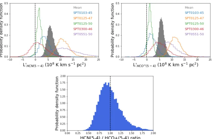
2.5. Unbiased average luminosities and line ratios
Given the relatively low line detection rate of our sample, we seek sample-averaged line luminosities and ratios without being biased towards the brightest sources. To this end, we used the bootstrap analysis results presented in Sect. 2.3. In Fig. 2, we illustrate our method in the case of the average HCN(5-4) and HCO+(5-4) luminosities and the flux ratio between these two lines. The probability density distribution (PDF) of the HCN(5-4) (upper left panels) and HCO+(5-4) (upper right panel) lumi-nosities of each source are represented as colored histograms. Concerning the >3σ lines of SPT0125-47 and SPT0551-50, their PDFs exclude clearly the null hypothesis (L0= 0) as is expected
for a (tentative) detection.
However, even for non-detections, the mode of the distribu-tion is systematically above zero. Since these PDFs are quasi-Gaussian, the mode is very close to the best-fit value. This is the case for the eight13CO(4-3), HCN(5-4), or HCO+(5-4) lines
present in our spectral windows. The case of HNC(5-4) and CN(4-3) is not discussed here but in Sect. 2.6, since they are blended and the interpretation is more complicated. If the lumi-nosity of these lines were strictly zero, the probability to have such a result would be (1/2)2= 0.3%, since there would be a 50%
chance for each individual PDF to have a negative mode. How-ever, their flux is unlikely to be zero and could correspond to 1– 3σ, since we planned our observation to attempt detections and the lines should not be too far from the detection threshold. Negative values of the mode of the distribution would thus be rather unlikely and would request a 1–3σ negative fluctuation of the noise in our observations. It is thus not so surprising that the modes of the PDFs of our non-detections are systematically positive. Indeed, the PDFs of such non-detections thus contain weak but potentially useful information, if we combine several objects. However, of course, these lines cannot be qualified individually as detections, since their PDFs do not exclude negative values and our measure-ments are thus compatible with a zero luminosity.
We determined the average luminosity of the sample using both detections and non-detections by combining their PDFs. Since our observations of each source are independent, we can assume that the measured luminosities are independent. The PDF of the sum of the luminosities of our sources can then be computed by convolving the PDFs of their individual luminosities,
1 The PhD manuscript ofYang(2017) can be downloaded athttps:
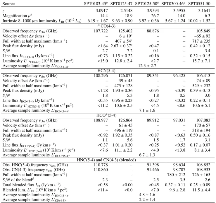
Table 2. Summary of the properties of our sources. Source SPT0103-45a SPT0125-47 SPT0125-50a SPT0300-46a SPT0551-50 z 3.0917 2.5148 3.9593 3.5955 3.1641 Magnification µb 14.4 18.9 26.7 14.0 6.3 Intrinsic 8–1000 µm luminosity LIR(1012L ) 6.19 ± 1.67 9.63 ± 0.90 3.92 ± 0.36 5.67 ± 1.24 10.02 ± 1.52 13CO(4-3)
Observed frequency νobs(GHz) 107.722 125.402 88.876 – 105.849
Velocity offset ∆ν (km s−1) – 6 ± 19e – – –65 ± 92
Full width at half maximum (km s−1) – 407 ± 54e – – 717 ± 235
Peak flux density (mJy) <1.64 2.67 ± 0.37e <0.47 – 0.42 ± 0.12
S/N 2.7 7.2 0.1 – 3.4
Line flux I13CO(4-3)(Jy km s−1) <0.73 1.15 ± 0.22 <0.16 – 0.32 ± 0.15
Luminosity L0
13CO(4-3)(108K km s−1pc2) <15.0 12.8 ± 2.4 <2.7 – 15.7 ± 7.1
Average sample luminosity L0
13CO(4-3)c 12.3 ± 2.7
HCN(5-4)
Observed frequency νobs(GHz) 108.296 126.071 89.351 96.425 106.413
Velocity offset ∆ν (km s−1) – 39 ± 45 – – 74 ± 89
Full width at half maximum (km s−1) – 475 ± 128 – – 529 ± 232
Peak flux density (mJy) <1.28 1.90 ± 0.36 <0.95 <0.39 0.39 ± 0.13
S/N 1.8 5.3 1.8 0.5 3.0
Line flux IHCN(5-4)(Jy km s−1) <0.55 0.96 ± 0.23 <0.27 <0.32 0.22 ± 0.11
Luminosity L0HCN(5-4)(108K km s−1pc2) <11.2 10.6 ± 2.5 <4.5 <8.6 10.6 ± 5.1
Average sample luminosity L0
HCN(5-4)c 7.1 ± 1.6
HCO+(5-4)
Observed frequency νobs(GHz) 108.977 126.864 89.912 97.031 107.083
Velocity offset ∆ν (km s−1) – 61 ± 45 – – 170 ± 57
Full width at half maximum (km s−1) – 496 ± 119 – – 318 ± 194
Peak flux density (mJy) <0.92 1.92 ± 0.35 <0.87 <0.63 0.50 ± 0.16
S/N 1.1 5.6 1.5 1.7 3.1
Line flux IHCO+(5-4)(Jy km s−1) <0.37 1.01 ± 0.20 <0.25 <0.52 0.17 ± 0.07
Luminosity L0HCO+(5-4)(108K km s−1pc2) <7.6 11.1 ± 2.2 <4.0 <13.8 8.1 ± 3.4
Average sample luminosity L0
HCO+(5-4)c 6.7 ± 1.3
HNC(5-4) and CN(4-3) (blended)
Obs. HNC(5-4) frequency νobs(GHz) 110.778 – 91.398 98.634 108.852
Obs. CN(4-3) frequency νobs(GHz) 110.860 – 91.466 98.707 108.933
Full width at half maximum (km s−1) – – – 780 ± 212 726 ± 165
S/N of the blendd 2.3 – 2.5 3.5 2.6
Total blended flux Itot(Jy km s−1) <0.58 <0.00 <0.45 0.37 ± 0.11 0.25 ± 0.09
Blended lum. L0
tot(108K km s−1pc2) <11.4 <0.0 <7.0 9.6 ± 2.8 11.5 ± 4.4
Average sample luminosity L0HNC(5-4)c 4.8 ± 1.6
Average sample luminosity L0CN(4-3)c 2.2 ± 1.4
Notes. We report the properties of lines of our detections and tentative detections (S /N ≥ 3). Upper limits correspond to 3σ. The blend between HNC(5-4) and CN(4-3) in SPT0551-50 can be considered as a tentative detection as justified in Fig.1and AppendixB.(a)We assumed the same
FWHM and∆ν for all lines to fit these low S/N sources.(b)The magnifications come fromSpilker et al.(2016). We have no good lens model for
SPT0551-50 and we thus assume the median magnification of the SPT sample of 6.3 (Spilker et al. 2016).(c)The average sample luminosity is
determined combining detections and non-detections using the method described in Sects.2.5and2.6.(d)The S/N of the blend of HCN(5-4) and
CN(4-3) is computed using the total flux of the two lines.(e)The13CO(4-3) line of SPT0125-47 is extracted assuming that the three lines have the
same width and velocity offset as discussed in Sect.2.3.
p N X k=1 L0k= N × hL0i = p1(L 0 1) ∗ p2(L02) ∗ . . . ∗ pN(L0N), (1)
where pi(L0i) is the PDF of the luminosity of the ith source.
The average is then computed by dividing this sum by N, the number of sources. In practice, we do not really need to com-pute this convolution analytically. We can just randomly draw luminosities from our 10 000 bootstrap realizations for each of our sources and then sum them. We performed this opera-tion 10 000 times to obtain the PDF of the average luminos-ity of the sample. In Fig. 2, the results are shown as gray
filled histograms. As expected, the width of the PDF of the mean luminosity is significantly narrower than the PDFs of individual objects. We can also remark that the mean lumi-nosity is clearly detected, since its PDF completely excludes zero.
We do not apply a positivity prior to perform our fits of the spectra. Indeed, in the hypothetical case of a line with a null flux for all sources, the bootstrap realizations would have a zero flux or a positive flux depending on the realization of the noise. The average flux would thus be positive even if the flux is zero for all sources. Practically, the absence of positivity prior would have
Fig. 2.Figures illustrating the method we used to derive unbiased average luminosity and line ratios (see Sect.2.5). Upper left panel: probability density distribution of the HCN(5-4) luminosity of our sources determined using a bootstrap technique (Sect.2.3). The gray filled histogram is the probability distribution of the mean luminosity of our five sources (see Sect.2.5). The vertical dashed line indicates the zero flux. Upper right panel: same figure for HCO+(5-4). Lower panel: probability density distribution of the ratio between the mean HCN(5-4) and the mean HCO+(5-4) luminosities. The vertical dashed line indicate the median value of the distribution.
a minor impact, since the probability of a negative flux is small (<10%), except for HCN(5-4) in SPT0300-46 and13CO(4-3) in SPT0125-50. Indeed, our unbiased mean luminosity estimates and the one derived with the positivity prior agree at better than 10%, that is, 0.5σ.
This method is close to a stacking method, except that we first measure noisy fluxes and then average them instead of the contrary. However, since the lines of the various sources have different widths and the baselines are difficult to subtract reli-ably, we preferred this approach to a standard stacking. Indeed, the stacked lines would have had a very peculiar shape, since these are the sum of lines with various widths. It would have been impossible to use our procedure to fit the lines and the baseline simultaneously. Finally, as explained in Appendix B, flux measurements based on stacked moment maps are also unreliable, since the baseline subtraction is potentially affected by biases due to the crowded spectral windows. A stacking procedure should not be used in this case, since the system-atic biases could be similar for all objects and this bias would stay roughly constant with the number of sources, while the noise would decrease in 1/√N. The measurement would thus be dominated by systematic effects and not the instrumental noise.
We used a very similar method to derive mean line flux ratios. We first computed the PDFs of the mean of the line fluxes from our bootstrap realizations using the same method as previ-ously described. However, to avoid giving more importance to low-z sources in the computation of the mean, we weighted the sources by the square of the luminosity distance. We then com-puted the ratio between these mean line fluxes. The PDF of the
ratio between two random variables is p r= hL 0 Ai hL0 Bi ! ∝ Z +∞ −∞ |X| pA(rX) pB(X) dX, (2)
where pA(rX) and pB(X) are the PDF of the flux of the line A and
B respectively, and r is the line ratio in luminosity. In practice, the uncertainties on the ratio are determined by drawing real-izations from the PDF of the mean luminosity of each line. The results are presented in Fig.2. The distribution is clearly asym-metric and we thus used the 16th and 84th percentile to produce the error bars in Table2. With this method, the contribution of the sources to the mean ratio is weighted by their luminosity. We tried to compute first the PDFs of the line flux ratios of individual sources and then average them, but this failed to get meaningful results. For low-S/N sources, the distribution is very broad with very large negative and positive outliers. Indeed, the PDF of the line flux in the denominator is compatible with zero and there are thus realizations for which the ratios are tending to+∞ or −∞. In AppendixC, we present the simulation used to validate this method.
2.6. Deblending of HNC(5-4) and CN(4-3) and determination of unbiased mean ratios
HNC(5-4) is blended with CN(4-3). To our knowledge, the only previous individual detection of this blend at high red-shift was performed byGuélin et al.(2007) in the lensed quasar APM 08279+5255 (see also Riechers et al. 2007b about the detection of CN(3-2) in the Cloverleaf). It is also detected in the stacked spectrum of all the SPT SMG sources observed
Table 3. Summary of the CO and [CI] data used in this paper. Source SPT0103-45 SPT0125-47 SPT0125-50 SPT0300-46 SPT0551-50 I12CO(4-3)(Jy km s−1) 11.7 ± 0.7 23.1 ± 0.6 7.9 ± 1.0 4.9 ± 0.5 12.0 ± 0.8 L0 12CO(4-3)(10 10K km s−1pc2) 2.22 ± 0.13 2.35 ± 0.06a 1.20 ± 0.15 1.22 ± 0.13 3.39 ± 0.24
Data origin Data from z-search programs (Weiß et al. 2013), fluxes fromBothwell et al.(2016)
ICI(1-0)(Jy km s−1) – 6.3 ± 0.2 2.4 ± 0.5 1.8 ± 0.8 –
L0CI(1-0)(intrinsic, 1010K km s−1pc2) – 0.56 ± 0.02 0.32 ± 0.07 0.39 ± 0.17 –
Data origin No data This paper z search (Bothwell et al. 2016) No data
Notes. All these data, except the new detection of [CI](1-0) in SPT0125-47, are ancillary and were extracted from the redshift-search program (Weiß et al. 2013) byBothwell et al.(2016).(a)Converted from the CO(3-2) flux using the mean flux ratio measured bySpilker et al.(2014) by
stacking.
by ALMA in cycle 0 (Spilker et al. 2014).Guélin et al.(2007) found that HNC(5-4) is 1.74 times brighter than CN(4-3) by fit-ting simultaneously the profile of the two lines in their spec-trum. This last source has a different nature than ours, but it shows that, even if HNC(5-4) might dominate the flux, the CN(4-3) contamination cannot be neglected. It is thus impor-tant to deblend the two lines in order to put a constraint on HNC(5-4).
To do so, we refitted the data with a slightly different method than the one described in Sect. 2.3. We fitted simultaneously all the lines in the spectrum including HNC(5-4) and CN(4-3) and forced all the lines to have the same width and velocity offset (including the sources with good S/N). The width and the velocity of the blended lines are thus strongly constrained by the other lines without being completely fixed. Since CN(4-3) and HNC(5-4) are not at the same exact frequency, these additional constraints are sufficient to extract information from the data. We also have to apply a positivity prior on the flux of HNC(5-4) and CN(4-3), since the degeneracies between the two fluxes tend to produce negative values to overfit noise pat-terns. Even under these assumptions, the uncertainties on the ratio for an individual source remain very high, with relative uncertainties higher than 50%. We thus derived the mean lumi-nosities of the two lines and the mean line flux ratio between HNC and CN using the method presented in Sect. 2.5. We found a mean HNC(5-4)/CN(4-3) ratio of 1.60+1.74−0.82. This value is close to the value found in the APM 08279+5255 quasar by
Guélin et al.(2007).
2.7. CO and [CI] lines extracted from ancillary data
We want to compare our dense-gas tracers with lines from cold gas at lower density (CO, [CI]) found by our previous red-shift search programs (Weiß et al. 2013; Strandet et al. 2016). The line fluxes of the [CI](1-0) line and the CO transitions covered by the redshift-search spectral scans were extracted in
Bothwell et al. (2016). For most of our sources, the CO(4-3) line falls in a frequency window covered by the redshift-search data. We thus chose to use this transition available for most of our sources as the reference one for CO in our analysis. For SPT0125-47, which is at lower redshift, only CO(3-2) is avail-able. We derived the expected CO(4-3) flux using the line ratio measured in the stacked spectrum of the SPT SMG sources derived by (Spilker et al. 2014), ICO(4-3)/ICO(3-2) = 0.7). Finally,
we detected [CI](1-0) in SPT0125-47 using our new ALMA data (see AppendixA). The ancillary data used in this paper are sum-marized in Table3.
3. Dense-gas tracers: HCN, HCO+, and HNC
3.1. Scaling relation between the HCN and HCO+flux and the infrared luminosity
The relation between the dense-gas content, traced by the HCN(1-0) line, and the SFR, traced by LIR, was found to be
linear in the local Universe byGao & Solomon (2004). A lin-ear correlation between LIR and L0HCN(1−0) is consistent with
the simple physical picture in which the giant molecular clouds (GMCs), traced by HCN, convert a fixed fraction of their mass into stars before being disrupted (e.g., Faucher-Giguère et al. 2013;Grudi´c et al. 2018). However, further studies found a sub-linear slope for the J = 3 − 2 transition (Bussmann et al. 2008;
Juneau et al. 2009), which could have an impact on the interpre-tation of the physics of the star formation in infrared-luminous objects and active galactic nuclei (AGN, e.g.,Narayanan et al. 2008a). More recently, after considering careful aperture cor-rections, Zhang et al. (2014) found a linear slope in the local Universe for the J = 4 − 3 transition. The LIR–L0CO relations
inferred for nearby galaxies have been found to be linear for J= 6 − 5 (Greve et al. 2014;Liu et al. 2015;Kamenetzky et al. 2016;Yang et al. 2017) and, possibly remain linear up to transi-tions as high as J = 12 − 11 (Liu et al. 2015). Extreme galax-ies, however, such as the local ULIRG population and high-z starbursts, show sublinear LIR–L0COrelations for J = 7 − 6 and
higher, due to large amounts of energy being injected, likely via mechanical heating, into a warm, dense, and non-star-forming ISM component (Greve et al. 2014;Kamenetzky et al. 2016).
At high redshift, the LIR–L0HCNrelation is poorly constrained
due to the small number of detections, all of which probe the high luminosity regime. However,Riechers et al.(2007a) con-cluded, based on the couple of detections and upper limits obtained at that time, that the LIR/L0HCN ratio must be higher in
high-z starbursts and quasars. This trend agrees with the theo-retical model of, for example, Krumholz & Thompson(2007), which predicts a superlinear trend for HCN and HCO+at high infrared luminosity. Similarly,Narayanan et al.(2011) predicted a similar superlinear trend for CO at very high LIR. According
to them, the median density of galaxies approaches the e ffec-tive density of the molecular tracers, and the LIR–Lmol relation
will approach the LIR–Mgas relation, which in both models has
a 1.5 exponent and is thus superlinear. On average, in high LIR systems such as DSFGs, the median gas density would be
much higher than in the lower luminosity systems investigated byGao & Solomon(2004) for which they found a linear trend.
To test if our galaxies follow the relation of Zhang et al.
(2014), we converted the L0
HCN(5-4)of our objects into L 0 HCN(4-3)
assuming the line ratio measured in the local Universe by (Mills et al. 2013), i.e., L0
HCN(5-4)/L 0
HCN(4-3)= 0.73), which is also
compatible with the measurements ofKnudsen et al.(2007) in NGC 253. We also corrected our sources for the magnification based onSpilker et al.(2016). The results are presented in Fig.3
(upper panel). In addition to our detections and upper limits (black squares), we also show the average L0
HCN(4-3)and LIR of
our sample (red stars). We also compared the mean properties of our sample with the mean L0
HCN(4-3)measured bySpilker et al.
(2014) from a stacked spectrum of six SPT sources in a slightly lower redshift range than our targets. To place their data in the diagram, we divided the mean L0
HCN(4-3) and LIR of their six
sources by their mean magnification, where a sample-median magnification of µ= 6.3 was assumed for sources with unknown magnification factor. Our new measurements are compatible with the previous results obtained by stacking.
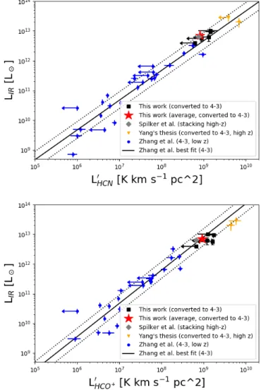
All our objects have a small deficit of HCN luminosity compared to the Zhang et al. (2014) relation (black line), per-haps similar to the deficit in HCN(2-1) relative to infrared (IR) observed in high-z quasars byRiechers et al.(2007a) (after accounting for the AGN contribution to the IR luminosity). This explains a posteriori why we did not reach our initial goal of 5σ detections in our four z > 3 sources (see Sect. 2.1). From theZhang et al.(2014) relation, we expect a mean L0HCN(5-4) of 11.1 × 10⁸K km s−1pc2 (after converting to the 5-4 transition)
based on the infrared luminosity of our sources. We measured an average flux of (7.1 ± 1.6) × 108K km s−1pc2. This corresponds
to a deficit by a factor of 1.6 (0.20 dex) corresponding to a 2.5σ difference. However,Zhang et al.(2014) used theSanders et al.
(2003) method to derive LIR, while another method was used for
the SPT SMG sample (Blain et al. 2003, model 1). We estimated the median factor between the two methods by fitting the pho-tometric points used byZhang et al.(2014) with the SPT SMG method. We found that their method derives luminosities that are a factor of 1.27 higher. When we take this into account, the ten-sion increases up to a factor of 2.0 (0.30 dex). In contrast, the HCN(5-4) detection of NCv1.143 and the upper limit towards G09v1.97 (provided by C. Yang) are both, when converted to HCN(4-3), consistent with the observed local relation.
We checked if the deficit found with our sample could be explained by sample variance. The scatter around the
Zhang et al. (2014) relation is ∼0.28 dex and we thus expect a 1σ sample variance for five objects of 0.28/
√
5= 0.125 dex. If we combine this with our measurement uncertainties, the signif-icance of the HCN deficit has thus only a ∼2σ signifsignif-icance. It is therefore not possible to draw any firm conclusions, especially considering the uncertainties involved in converting our HCN(5-4) fluxes to HCN(4-3). Apart from intrinsic scatter in the 5-4/4-3 ratio, systematic effects could also be introduced by applying a locally-determined ratio to high-z starburst galaxies. More data will be needed in the future.
We performed a similar analysis for the HCO+. The conver-sion factor from the 5-4 to the 4-3 transition based onMills et al.
(2013) is 0.64. Our results agree with theZhang et al.(2014)2 relation (see Fig. 3, lower panel) and the average properties of our sources agree with the measurements by stacking of
Spilker et al.(2014). Based on the Zhang et al.(2014) relation and the mean infrared luminosity of our sample, we expect a mean L0HCO+(5-4) of 6.9 × 10
8K km s−1pc2 (after applying the
2 There is a small mistake inZhang et al.(2014) and they provided us
with an updated relation (priv. comm.), which we used in our analysis: log(LIR)= 1.12 log(L0HCO+(5-4))+ 2.83.
Fig. 3.Upper panel: scaling relation between the HCN(4-3) luminos-ity (converted from 5-4, see Sect.3.1) and the total infrared luminosity. The black squares are the individual values found in our high-z sample (after correcting for the lensing magnification). The red star shows the average intrinsic L0
HCNand LIRof our sample. The gray diamond is the
mean position of the SPT SMG sample derived from the stacking of the ALMA cycle-0 data bySpilker et al.(2014). The orange downwards tri-angles are two H-ATLAS sources provided in Yang et al. (priv. comm.). The blue filled circles are from the local sample ofZhang et al.(2014). The black solid line is the best-fit relation ofZhang et al.(2014) and the dotted lines indicate the 1σ intrinsic scatter around it. Lower panel: same figure but for HCO+.
correction to homogenize the LIR, see above) and we found
(6.7 ± 1.3) × 108K km s−1pc2, which is in excellent agreement. Within the scatter, the HCO+detections provided by C. Yang are also in agreement with the relation.
3.2. The HCO+to HCN flux ratio
We compared the HCO+/HCN J = 5 − 4 flux ratios of our SPT sources (see Table4) with HCO+/HCN ratios of low- and high-z galaxies from the literature (Fig.4). The main advantage of using flux ratios is that they cancel out the magnification factor µ if the differential magnification (Hezaveh et al. 2012;Serjeant 2012) is negligible (see Sect. 4.3). While some of the HCO+/HCN ratios from the literature were for transitions other than J = 5 − 4, we proceeded to compare them with our ratios under the assumption that the spectral line energy distributions (SLEDs)
Table 4. Line flux ratios measured in our sources.
Line flux ratio SPT0103-45 SPT0125-47 SPT0125-50 SPT0300-46 SPT0551-50 Mean ratio
IHCO+(5-4)/IHCN(5-4) – 1.05−0.24+0.30 – – 0.78+0.49−0.28 1.00+0.23−0.19 IHNC(5-4)/ICN(4-3) – – – – – 1.60+1.74−0.82 IHNC(5-4)/IHCN(5-4) – – – – – 1.03+0.59−0.39 I12CO(4-3)/I13CO(4-3) >10.9 19.7+4.0 −3.1 >23.1 – 33.7+21.1−10.9 26.1+4.5−3.5 IHCN(5-4)/I12CO(4-3) <0.067 0.043+0.010 −0.009 <0.055 <0.095 0.020+0.010−0.008 0.030+0.006−0.005 IHCN(5-4)/I[CI](1-0) – 0.158+0.038−0.032 <0.215 <1.374 – 0.129+0.031−0.026
Notes. The mean ratio is computed combining all the sources for which these two lines were observed (see the description of the method in Sects.2.5and 2.6). For the ratios between two dense-gas tracers, we provided values only when the two lines are detected at more than 2σ. Otherwise, the ratio is often compatible at 2σ with both zero and infinity. Concerning the12CO/13CO, only SPT0125-50 is observed and not
detected and we consequently derived a lower limit on this ratio, since12CO is well detected. For the ratio between HCN(5-4) and CO(4-3) or
[CI](1-0), we derived upper limits, since the denominator (CO or [CI]) is often detected.
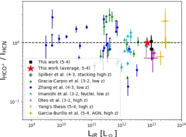
Fig. 4. Line flux ratio between HCO+ and HCN as a function of the infrared luminosity. The black squares are the individual values obtained for our sources (only sources with two >3σ lines are shown) and the red star is the average value of our five objects. The gray dia-mond is the mean ratio found bySpilker et al.(2014) using a stack-ing of the cycle-0 SPT SMG spectra. The green triangles are the ratios of the 3-2 transitions in the local sample ofGraciá-Carpio et al. (2008) and blue filled circles are the 4-3 ratios in the low-z sample of Zhang et al.(2014). The cyan pentagons represent the 3-2 ratios mea-sured in local active nuclei byImanishi et al.(2016). The purple crosses shows the 3-2 ratio measured in z ∼ 1.5 lensed star-forming galax-ies by Oteo et al.(2016). The orange downwards-facing triangles are two H-ATLAS sources provided by Yang et al. (priv. comm.). The yel-low plus is the 5-4 flux ratio found byGarcía-Burillo et al.(2006) in the APM08279+5255 quasar (see alsoRiechers et al. 2010for the 6-5 transition).
of the HCO+ and HCN are similar. In addition to the average value (1.00+0.23−0.19) of our sample, we put in our diagram only the sources that have at least a 3σ signal at the position of each line (SPT0125-47 and SPT0551-50). For the other sources with <3σ signal, both the numerator (HCO+flux) and the
denomina-tor (HCN flux) are compatible with zero at 3σ (see Sect. 2.5). The PDF of their ratio is thus compatible with both zero and infinity at 3σ and deriving upper or lower limits does not make sense. Nevertheless, we checked the average line ratio derived for these three other sources and found that it is compatible at 1σ with the average value derived for the fives sources and the two individual measurements, but with very large uncertainties (0.98+0.73−0.40).
Similar to the local star-forming samples of
Graciá-Carpio et al. (2008) and Zhang et al. (2014), the mean ratio of our sample is compatible with unity. This is con-sistent with the ratio derived for the J = 4 − 3 transitions using the stacked spectra ofSpilker et al. (2014), but with improved uncertainties. The mean ratio of our sample is 2σ higher than in the two high-z star-forming galaxies of Oteo et al. (2016). NCv1.143 (Yang et al.) has similar values to these two objects, but G09v1.97 has a much higher value (∼2). However, all these high-z sources are in the intrinsic scatter of the local relation. As in the low-z Universe, the ratio varies significantly within the population of lensed DSFGs.Braine et al.(2017) found that low-metallicity regions of local galaxies (<0.5 Z ) have a high
HCO+/HCN flux ratio (∼2) instead of a ratio close to unity. Finding a unity ratio in our sources could be consistent with an already mature ISM at early cosmic times, but a larger statistical sample will be necessary to confirm or not this possibility.
Recently, Imanishi et al. (2016) and Izumi et al. (2016) found a HCO+/HCN flux ratio (∼0.5) for both the J = 3 − 2 and J = 4 − 3 transitions that is lower in local AGNs than in star-forming galaxies3 and proposed that this quantity could be used to identify AGNs. Izumi et al. (2016) discussed two explanations for the low HCO+/HCN: an enhanced abundance of HCN compared with HCO+coming from the complex chem-ical and radiative mechanisms involving these molecules in the neighborhood of an AGN or a systematically higher gas density around AGNs. We found a ratio close to unity, which is consis-tent with our objects being star-formation dominated. However, we should interpret this simple diagnostic with caution, since some AGNs ofImanishi et al.(2016) and the APM08279+5255 quasar at z= 3.9 have flux ratios close to unity.
3.3. The HNC to HCN flux ratio
Other important diagnostics can be performed using the isomer ratio between HNC and HCN. HNC traces gas of similar density to HCN, but the observed HNC/HCN flux ratio is close to unity in dark clouds and up to 100 times smaller in hot environments (Schilke et al. 1992;Hirota et al. 1998). In addition,Aalto et al.
(2007) showed that the HNC/HCN flux ratio can be above unity in local starbursts, which is not intuitive because HNC should be more easily destroyed than HCN by the strong radiation fields and high temperatures in these objects. They proposed
3 In the original articles, the authors used the HCN/HCO+flux ratio
(the inverse) and thus discussed a high ratio instead of a low ratio in this paper.
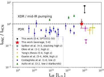
Fig. 5. Line flux ratio between HNC and HCN as a function of the infrared luminosity. The red star is the mean ratio found in our sources and the gray diamond is the mean ratio found bySpilker et al.(2014) using a stacking of the cycle-0 SPT SMG spectra. The black square is the upper limit determined for SPT0551-50. For the other sources, the individual ratio cannot be constrained, since both lines are too weak to derive an upper or a lower limit. The blue filled circles represent the local sample of (Costagliola et al. 2011, 1-0 transition). The green trian-gles are the 3-2 transitions in the Arp220, Mrk231, and NGC4418 star-bursts (Aalto et al. 2007). The purple crosses are the two z ∼ 1.5 lensed star-forming galaxies ofOteo et al.(2016) and the yellow plus is the APM08279+5255 quasar (Guélin et al. 2007, see alsoRiechers et al. 2010for the 6-5 transition). The orange downwards triangles are two H-ATLAS sources provided in Yang’s Thesis (priv. comm.).
two possible explanations: HNC is excited by mid-IR pump-ing of its rotational levels or X-ray dissociation regions (XDRs) have an impact on the abundance of HNC. Since then, the case of Arp220 has been extensively investigated and more signs of HCN or HNC pumping have been identified (e.g., Aalto et al. 2015;Galametz et al. 2016). Finally, a similar scenario was also discussed inWeiß et al.(2007) to explain HCN luminosity in the high-redshift quasar APM08279+5255.
Because of the blending of HNC(5-4) with CN(4-3), we derived only a mean HNC/HCN ratio using the method described in Sect.2.6, and found a ratio compatible with unity (1.03+0.59−0.39). This ratio is compatible with the one obtained by stacking of the HNC(4-3) and HCN(4-3) lines by (Spilker et al. 2014, gray dia-mond in Fig.5). Since the HCN(4-3) line is not blended, it is thus reassuring to find similar values. Our sources are at the bor-der between the regime dominated by photodissociation regions (PDRs) and the domain, where XDR and/or mid-IR pumping are necessary to explain the line ratios. In Fig.5, we compare the mean ratio found for our sample (derived using the method described in Sect.2.6) with local and distant samples. The mean HNC/HCN ratio of our sample is a factor of approximately three above the local IRAM/30 m sample ofCostagliola et al.(2011), but lower by a factor of approximately two than the starbursts of Aalto et al. (2007). Our average measurements are only 1σ above the measurements of APM08279+5255 byGuélin et al.
(2007), SDP.9 of Oteo et al. (2017), and NCv1.143 in Yang’s Thesis, but an order of magnitude above the upper limit for SDP.11 (Oteo et al. 2017).
4. Dense gas versus lower density tracers (CO, [CI]) The origin of the strong star formation in the most extreme high-redshift starbursts is a source of intense debates (e.g.,
Engel et al. 2010; Daddi et al. 2010; Hayward et al. 2011,
2013;Carilli & Walter 2013;Casey et al. 2014;Narayanan et al. 2015). Large gas reservoirs are not sufficient to explain the SFR
of the most extreme systems and a temporary increase of the star formation efficiency, measured relative to the total gas mass as traced by CO(1-0) or CO(2-1), is necessary (e.g.,Daddi et al. 2010;Genzel et al. 2010;Sargent et al. 2014).Gao et al.(2007) andDaddi et al.(2010) suggested that the increase of the star for-mation efficiency in these objects is linked to an increase of the dense-gas fraction (DGF). The dense gas fraction is thus one of the keys to understanding the nature of this type of sources. We note, however, that an increase in the dense-gas star formation efficiency is not required in this picture.
4.1. Dense gas fraction versus infrared luminosity
In this section we compare the flux ratio between HCN(5-4), which probes the dense gas, and [CI](1-0), which is thought to be a tracer of the bulk gas reservoir. For the three sources in our sample with [CI](1-0) measurements, we therefore adopt this ratio as a proxy for the DGF.
To build a reference sample in the local Universe, we combined the HCN(4-3) sample of Zhang et al. (2014) with the [CI] fluxes from the local Herschel/spectral and pho-tometric imaging receiver (SPIRE) spectroscopic sample of
Rosenberg et al.(2015). We adopted the aperture-corrected inte-grated [CI] fluxes published by Rosenberg et al. (2015), and, similarly, the aperture-corrected integrated HCN(4-3) fluxes published byZhang et al.(2014). Finally, the HCN(4-3) fluxes were converted into HCN(5-4) using the conversion described in Sect.3.1.
In the left panel of Fig.6, we show the ratio between HCN (5-4) and [CI](1-0) versus LIR for our three sources observed
in [Ci](1-0). Also shown is their mean flux ratio, as well as the upper limit derived from the stacked spectra of SPT sources (Spilker et al. 2014). Our sources are seen to be consistent with the stacked SPT value, but at the limit of the upper envelope of the local reference sample.
Given the lack of low-J CO transitions for some of our sources, we are not able to gauge the dense gas fraction using HCN(mid-J)/CO(low-J) ratio. Instead we opted for the J = 4−3 CO transition, since it is available for most of our sources, and examine the HCN(4-3)/CO(4-3) ratio. HCN(4-3) and CO(4-3) have similar upper level energies (EJ/kB ∼ 40−55 K) and both
trace dense gas, albeit HCN(4-3) has a ∼400 × higher criti-cal density than CO(4-3) (∼8 × 106cm−3 vs. ∼104cm−3). For the local reference sample we again adoptZhang et al.(2014), and use their directly measured HCN(4-3) fluxes and the CO (4-3) fluxes from Rosenberg et al. (2015) to form the HCN(4-3)/CO(4-3) ratios. In the right panel of Fig. 6, we compare the HCN(4-3)/CO(4-3) flux ratios of our sources, where we have converted HCN(5-4) to HCN(4-3). There are not a lot of HCN(4-3)/CO(4-3) measurements of high-z sources avail-able in the literature, and we therefore extended our compari-son to HCN(5-4)/CO(5-4) and HCN(3-2)/CO(3-2) in order to facilitate a comparison with other high-z starbursts. Our mean HCN(4-3)/CO(4-3) ratio is in the scatter of the local values and compatible with the upper limit on G09v1.97 (Yang’s The-sis). In contrast, our sources are on average a factor of 1.6 lower than the stacking measurement of Spilker et al. (2014) on the full cycle-0 SPT SMG sample (∼2σ difference) and a factor of approximately three below the high-z measurements ofOteo et al.(2016) in SDP.9,Danielson et al.(2011) in SMM J2135-0102, and NCv1.143 in Yang’s Thesis.
Fig. 6.Left panel: flux ratio between HCN(5-4) and [CI](1-0) as a function of the infrared luminosity. Our sources are represented by black filled squares and the average by a red star. The gray diamond represents the stacking of the cycle-0 SPT SMG spectra (Spilker et al. 2014). The blue filled circles are the local HCN(4-3) measurements ofZhang et al.(2014), where HCN(4-3) is converted into HCN(5-4) following the recipe described in Sect.3.1, combined with the [CI](1-0) measurements ofRosenberg et al.(2015). Right panel: ratio between HCN(4-3) and
12CO(4-3) as a function of the infrared luminosity. As explained in Sect.4.1, we used the HCN(5-4)/CO(5-4) or HCN(3-2)/CO(3-2) ratios, when
the 4-3 transitions were not available. The purple cross is the measurement ofOteo et al.(2016) in SDP.9. The orange downwards triangles are two H-ATLAS sources provided in Yang’s Thesis (priv. comm.). The yellow triangle is the measurements ofDanielson et al.(2011) in SMM J2135-0102.
Fig. 7.Ratio between HCN(5-4) and [CI](1-0), tracing the dense-gas fraction, as a function of the ratio between the infrared and the [CI](1-0) luminosity, tracing the star formation efficiency. The data comes from the same references as in Fig.6. The red solid line is a linear relation between the dense-gas fraction and the star formation efficiency (DGF ∝ SFE), which normalization has been set to match the mean value of our sample (red star).
4.2. A link between dense-gas fraction and star formation efficiency
Gao et al.(2007) found a correlation between L0
HCN(1-0)/L 0 CO(1-0)
and LIR/L0CO(1-0), which they interpreted as a correlation between
the DGF and the SFE (with respect to the total gas mass). In Fig. 7, we performed a similar diagnostic using [CI](1-0) instead of CO(1-0) and HCN(5-4) instead of HCN(1-0). Our SPT sources are consistent with the trend of DGF versus SFE found in our local reference sample described in Sect. 4.1. A similar result is found if we use CO(4-3) instead of [CI](1-0) (see Fig.D.1). This seems to indicate that the correlation between the DGF and the SFE is still valid for the most star-forming systems
at high redshift and for the densest gas probed by the high-J tran-sitions of HCN. However, an artificial correlation can appear in diagrams representing A/C versus B/C. In AppendixD, we con-firm that it is not the case for our analysis using two different total gas mass tracers in the x and y axis.
The relation linking our local reference sample and the SPT sources suggests that DGF ∝ SFE (solid red line in Fig. 7). This result agrees with the suggestion byGao et al.(2007) and
Daddi et al.(2010) that the high SFEs in starbursts are directly connected to their DGF. The link between these two quantities is not surprising, if, as suggested by the various physical models cited previously, the amount of dense gas, rather than the total gas reservoir, drives the SFR. Unfortunately, our observations do not allow us to form a conclusion about the mechanism that causes these high DGFs. The sources in our sample are at the high end of the SFE and DGF distribution of our local reference sample. Their impressive SFRs are thus caused by a combination of large gas reservoirs (Aravena et al. 2016) coupled with a high DGF.
4.3. Similarity of the line profiles in SPT0125-47 and differential lensing
In SPT0125-47, dense-gas tracers are detected at more than 5σ and it is thus possible to compare the line profile of HCN and HCO+with [CI] and CO (see Fig.8). Our high-S/N [CI] detec-tion and the ancillary CO(3-2) line detecdetec-tion from the redshift search have a similar asymmetric profile with a much broader redshifted tail. A similar asymmetry is found for HCN(5-4) and HCO+(5-4). This suggests that molecular regions from the low-est to the highlow-est density are distributed in the same way across this object.
The similarity of the profiles also suggests that differential lensing (Hezaveh et al. 2012;Serjeant 2012) should not be too strong in this object. Concerning the other objects of our sam-ple, we do not have a sufficient S/N to be able to check the sim-ilarity of the profiles between the12CO lines and the dense-gas
Fig. 8. Comparison of the velocity profile of the dense-gas lines (HCN(5-4) in blue solid line and HCO+(5-4) in red dashed line, and other gas tracers (CO(3-2) in green dotted line and [CI](1-0) in yellow dot-dash line. We plotted the channel RMS uncertainties of HCN(5-4). HCO+(5-4) has similar channel uncertainties (not plotted).12CO and
[CI] have a much better S/N and their uncertainties can be neglected. We normalized all the lines to haveR Sνdν= 500 Jy km s−1. With this
nor-malization, the peak flux of a rectangular line with a typical 500 km s−1
width is unity.
the SPT sources have for instance similar CO and [CII] profiles. Except if the dense-gas lines have a fundamentally different spa-tial distribution than lower density tracers, we have no good rea-son to expect a priori any strong differential lensing effect. We thus neglected this effect in this paper. The only way to measure the impact of the differential lensing on integrated fluxes would be to perform high-resolution imaging of dense-gas lines, but it is out of reach of ALMA in a reasonable amount of time. 5. Properties of the CO isotopic lines
5.1. Flux ratios between13CO and12CO
As explained in the Introduction, the [12C]/[13C] abundance ratio
has been proposed as a diagnostic of the evolutionary stage of a galaxy, since different nuclear reactions produce12C and13C; the
former is produced via triple alpha nuclear processes in young massive stars, while the latter is produced in the CNO cycle in evolved asymptotic giant branch (AGB) stars (Wilson & Rood 1994).
A high [12C]/[13C] abundance ratio, therefore, could indicate
a chemically young and largely unprocessed ISM (Hughes et al. 2008;Henkel et al. 2010). However, other physical mechanisms could result in a high [12C]/[13C] ratio, namely star formation from a top-heavy IMF in young starbursts (e.g., Romano et al. 2017; Zhang et al. 2018) – with the latter being the result of extreme cosmic-ray-dominated, star formation regions rather than a metal-poor gas. In intense starburst environments, the cos-mic ray heating may be so severe that dense, deeply embedded molecular cores are significantly heated, resulting in a raise of the Jeans mass floor (Papadopoulos et al. 2011).
The [12C]/[13C] ratio is typically constrained indirectly from
observations of CO, HCN, and HCO+ and their 13C topologues. This approach, however, is complicated by iso-tope fractionation where chemical reactions involving 13C are
energetically favored over the same reactions involving 12C (Watson et al. 1976;Langer et al. 1984). The expectation from
Fig. 9.Flux ratio between the 13CO and 12CO as a function of the
infrared luminosity. The same transition of both lines is used to com-pute these ratios. Our sources are represented by black filled squares and their average properties by a red star. The two serendipitous detec-tions obtained during the first redshift-search campaign in SPT0529-54 and SPT0532-50 (Weiß et al. 2013) are shown using orange pentagons. The gray diamond shows the average ratio measured bySpilker et al. (2014) using a stacking of the full redshift-search SPT sample. The local sample fromCostagliola et al.(2011) is plotted with a blue filled circle. The yellow triangle and the green cross are the high-z measurements of Danielson et al.(2013) in SMM J2135-0102 andHenkel et al.(2010) in the Cloverleaf quasar.
isotope fractionation is that [12CO]/[13CO] provides a lower limit to [12C]/[13C] (Langer et al. 1984;Tunnard & Greve 2016).
Furthermore, in intense far-UV environments, selective pho-todissociation can lead to an increase in [12CO]/[13CO], since 13CO is readily destroyed given its low abundance, while12CO
will be able to self-shield (Bally & Langer 1982). However, this effect is expected to play a role only in diffuse gas (AV∼1) and it
is thus doubtful whether selective photodissociation plays a sig-nificant role in dusty galaxies, where FUV light undergoes heavy extinction (Casoli et al. 1992;Papadopoulos et al. 2014).
Finally, it is non-trivial to infer 12CO-to-13CO abundance
ratios from their line intensity ratios. This is because the12CO lines are optically thick, while the rarer 13CO lines tend to be
optically thin (e.g.,Casoli et al. 1992;Aalto et al. 1995). Optical depth effects can thus complicate the picture, since in the case where12CO is optically thick the12CO/13CO line intensity ratio
will be an upper limit to the [12CO]/[13CO] abundance ratio. In Fig.9(left), we compare our measurements of the12CO
versus13CO ratio with the literature. We found a mean ratio of 26.1+4.5−3.5, which is two times higher than the measurements of
Spilker et al.(2014) using the stacked spectra of all SPT SMGs observed by ALMA during the cycle 0. Our sample was selected because of their high apparent luminosity and could be biased towards objects with a stronger contribution of the recent star formation to the ISM enrichment. It is therefore not surprising to find a lower13CO abundance, and thus a higher12CO/13CO ratio, in our subsample.Weiß et al.(2013) reported a detection of
13CO(4-3) in SPT0529-54 and a tentative detection in
SPT0532-50 in the initial SPT SMG redshift-search program. The fluxes of these two lines, not published in the original paper, are 1.36 ± 0.24 Jy km s−1and 1.07 ± 0.32 Jy km s−1, respectively, while the 12CO(4-3) fluxes are 8.32 ± 0.34 Jy km s−1 and 14.89 ±
0.41 Jy km s−1. These two sources have much lower ratios than the new objects presented in this paper. This is not surprising,
![Table 3. Summary of the CO and [CI] data used in this paper.](https://thumb-eu.123doks.com/thumbv2/123doknet/14785930.598796/9.892.67.831.153.294/table-summary-ci-data-used-paper.webp)
, tracing the dense-gas fraction, as a function of the ratio between the infrared and the [CI](1-0) luminosity, tracing the star formation efficiency](https://thumb-eu.123doks.com/thumbv2/123doknet/14785930.598796/13.892.63.430.553.817/tracing-fraction-function-infrared-luminosity-tracing-formation-efficiency.webp)
 in yellow dot-dash line](https://thumb-eu.123doks.com/thumbv2/123doknet/14785930.598796/14.892.463.830.123.390/comparison-velocity-profile-dense-dashed-tracers-dotted-yellow.webp)