Empirical reconstruction of salinity from temperature profiles with phenomenological constraints

(1)

HAL Id: hal-00298460

https://hal.archives-ouvertes.fr/hal-00298460

Submitted on 3 Jan 2007

HAL is a multi-disciplinary open access

archive for the deposit and dissemination of sci-entific research documents, whether they are pub-lished or not. The documents may come from teaching and research institutions in France or abroad, or from public or private research centers.

L’archive ouverte pluridisciplinaire HAL, est destinée au dépôt et à la diffusion de documents scientifiques de niveau recherche, publiés ou non, émanant des établissements d’enseignement et de recherche français ou étrangers, des laboratoires publics ou privés.

Empirical reconstruction of salinity from temperature

profiles with phenomenological constraints

F. Reseghetti

To cite this version:

F. Reseghetti. Empirical reconstruction of salinity from temperature profiles with phenomenological constraints. Ocean Science Discussions, European Geosciences Union, 2007, 4 (1), pp.1-39. �hal-00298460�

(2)

OSD

4, 1–39, 2007 Estimate of salinity from temperature profiles F. Reseghetti Title Page Abstract Introduction Conclusions References Tables Figures ◭ ◮ ◭ ◮ Back Close

Full Screen / Esc

Printer-friendly Version Interactive Discussion

EGU Ocean Sci. Discuss., 4, 1–39, 2007

www.ocean-sci-discuss.net/4/1/2007/ © Author(s) 2007. This work is licensed under a Creative Commons License.

Ocean Science Discussions

Papers published in Ocean Science Discussions are under open-access review for the journal Ocean Science

Empirical reconstruction of salinity from

temperature profiles with

phenomenological constraints

F. Reseghetti

ENEA-ACS CLIM-MED, Forte S. Teresa – Pozzuolo di Lerici, 19032 Lerici (Sp), Italia Received: 26 October 2006 – Accepted: 11 December 2006 – Published: 3 January 2007 Correspondence to: F. Reseghetti (reseghetti@santateresa.enea.it)

(3)

OSD

Full Screen / Esc

Abstract

The problem of estimating the salinity when only temperature profiles are available is having an increasing interest mainly because of multi-parametric data assimilation in ocean forecasting models. In this paper, a new method based on the introduction of a correction factor for salinity deduced from recent measurements is proposed to

cal-5

culate salinity from temperature profiles and climatological datasets. It is supposed that the seawater potential density in a specific area, as deduced from climatological monthly averaged temperature and salinity values, does not change. A certain but small variability on its values is admitted and estimated combining the uncertainty of temperature and salinity in-situ measurements, and the diurnal variation, as obtained

10

from a set of recent CTD and MedArgo measurements in Tyrrhenian Sea. Then, the deduced range of variability for salinity and potential density is imposed to synthetic values, which are compared with CTD and XCTD data. Finally, this technique is used to calculate salinity profiles from XBT temperature profiles from Ligurian and Tyrrhe-nian Sea (XBT probes monthly dropped along the transect Genova-Palermo, within

15

the Mediterranean Forecasting System-Toward Experimental Prediction project). Re-sults are analysed and discussed.

1 Introduction

Measurements of seawater temperature (T ) are much easier to do and cheaper than the ones of salinity (S). Ships of opportunity have collected a wide amount of

tem-20

perature profiles, and, consequently, the dataset of temperature values is much bigger than the salinity dataset. The implementation of multi-parametric data assimilation schemes in ocean forecasting models implies the use of realistic S values estimated from T profiles. The usual way-out is based on climatological datasets and some phys-ical assumptions.

25

(4)

OSD

Full Screen / Esc

EGU

T and S values, but the relationship among salinity, temperature and other variables changes from region to region (Emery and Dewar, 1982), and was used for determining water types since early 40’s (Sverdrup et al., 1942). It is useful to introduce the potential temperature (θ) values. It is possible to estimate salinity or potential density (σ) from T profiles, but this is not a very difficult task only where seawater regimes are well known

5

and stable. Under the assumption that a certain θ-S relationship does exist (even if changing in time and space), many authors proposed different techniques in order to calculate S profiles and/or dynamic heights when only T profiles are available, as from XBT measurements (e.g. Hansen and Thacker, 1999).

Among several approaches, Sverdrup et al. (1942) proposed to adopt a straight-line

10

T-S representation using end-points for the North Atlantic Central Water, by assuming that intermediate temperature water has salinity value on the straight line. Stommel (1947) supposed that the main part of salinity variability is due to vertical movements of water having that S and T values. Then, he proposed that the expected salinity at a given temperature is more or less the value previously measured at the same

15

temperature.

Emery (1975) utilised mean θ-S diagrams to obtain the salinity corresponding to a measured temperature. Emery and O’Brien (1978) suggested a mean pressure – salinity relationship, in which S was derived from T , and mean local P-S curves; the authors were also able to calculate more accurate geo-potential heights than

Stom-20

mel’s method did. An early version of this approach was developed in Emery and Wert (1976), whereas different upgrades were done in Emery and Dewar (1982), and in Siedler and Stramma (1982). Donguy et al. (1986) introduced in their computations sea surface salinity as deduced from θ-S relationship. The near-surface portion was defined by linear interpolation from T and S monthly average values at surface to the

25

subsurface S maximum, which is usually present in tropical Pacific Ocean, and, one year later, Kessler and Taft (1987) improved this method. K ¨ase et al. (1996) developed a method based on observed horizontal distribution of T and S profiles; they were able to reproduce T and S variations at constant pressure over distance in case of smooth

(5)

OSD

Full Screen / Esc

and monotonic changes between CTD stations. Hansen and Thacker (1999) upgraded the Emery and O’Brien’s (1978) proposal, and computed the coefficients relating the estimated S profile with measured “predictor parameters” (T, sea surface salinity, and latitude) by usinga fitting procedure. From the analysis of the influence of assimilation within models, Troccoli and Haines (1999) proposed to derive a T -S relationship from

5

the most recent data in proximity of each T profile, or from the model (Haines et al., 2005).

Each approach presents some problems. Following K ¨ase et al. (1996), the method of Emery and Dewar (1982) can produce large errors in salinity values in regions with mesoscale variability and water mass conversions, and it is not suitable if large

anoma-10

lies occur. On the other hand, the Sverdrup et al. (1942) method fails in situations where T and salinity do not have a one-to-one correspondence within a T -S relation-ship.

Empirical Orthogonal Function (EOF) decomposition of historical T and S data of-fers a completely different way-out: S is reconstructed from a linear combination of

15

the dominant modes. The coefficients are obtained by minimising the difference be-tween modes and data from available observations, namely T and sea level (see Maes, 1999; Maes and Behringer, 2000, and references therein; Maes et al., 2000). Carnes et al. (1994) proposed regression models estimating the coefficients of salinity EOFs from the coefficients of temperature EOFs. Vossepoel et al. (1999) presented a hybrid

20

method, estimating S below the bottom of thermally mixed layer by T-S technique and within the isothermal layer by linear interpolation to a measured sea surface salinity. When a great anomaly occurs, this technique produces fictitious density inversions; therefore a correction, using sea surface heights, mainly from satellite observations, is introduced.

25

Most of the cited authors (e.g. Vossepoel et al., 1999) showed that σ profiles cal-culated by means of the synthetic salinity are not guaranteed to be close to the true potential density, but the “mean computed value” is in a good agreement with the “true mean value”, due to compensations in the vertical profile. Therefore, the computed

(6)

OSD

Full Screen / Esc

EGU surface geo-strophic currents, and dynamical heights are quantitatively good, even if

problems arise when a more complete description of the internal dynamics is required. Recently, the calculation of salinity from T profiles became of paramount importance for the ocean forecasting (e.g. De Mey and Benkiran, 2002) because of multivariate assimilation in numerical models (Demirov et al., 2003; Sparnocchia et al., 2003): in

5

fact, multivariate data assimilation greatly improves the models. In this regard, XBT data are operationally collected, and S profiles are calculated by using historical data, and EOF technique.

MODAS (Modular Ocean Data Assimilation System) approach (Fox et al., 2002) combines the Hansen and Thacker technique (in order to estimate salinity from XBT

10

profiles) with regression models assuming that climatological T and S values agree with observed T -S relationships. More in detail, salinity is computed by a linear func-tion of temperature with coefficients depending on specific area and depth. Recent improvements, i.e. HYCOM (Hybrid-coordinate Ocean Model), see Bleck (2002), and Halliwell (2004), try to include XBT data into the model (Thacker and Esenkov, 2002),

15

and to extend initial steps based on Gulf of Mexico analyses to open oceans such as Atlantic Ocean (Thacker, 2006, Thacker and Sindlinger, 2006).

The different techniques are based on the underlying idea that the relationship be-tween T and S for certain sea areas is seasonally changing, but it shows very small variations over longer time scales, with the “natural” exception of near surface

seawa-20

ter. In many cases, this is a good working hypothesis, but the reliability of the above-mentioned methods is not assured in areas where the seawater physical characteristics are subjected to a high inter-annual variability. This is the case of Mediterranean Sea, having great and rapid changes, a non-simple behaviour probably related to its size, coastal influences, and bathymetry.

25

Some processes producing temperature instability are not correlated to salinity vari-ability: examples were provided in areas of strong mixing, such as the surface mixed layers, or eddy induced mixing. The θ-S relationship cannot be well defined, and can be strongly time-dependent in isothermal layers presenting salinity stratification. For

(7)

OSD

Full Screen / Esc

example, Hansen and Thacker (1999) found that CTD profiles from Pacific Ocean show a depth-dependent behaviour: local correlation between θ and S is small in the upper 50 m, small and negative between 50 and 150 m depth, positive below 200 m. It must be noted that θ and S temporal variability decreases with depth; moreover, the θ-S relationships derived from climatological datasets (when and where climatology is

rep-5

resentative of an averaged state), are generally valid, and remain almost unchanged over the time. Therefore, they can be used as an approximation estimating salinity from temperature values. Salinity on pressure surfaces at a fixed date can be reproduced in an approximate way by a function of temperature and geographic coordinates (i.e. linear function in MODAS). The use of high degree polynomial of temperature,

coordi-10

nates, pressure, and so on, does not improve the results as expected. In fact, specific (local) values of data used to compute the coefficients of the polynomial could induce a rough description of independent data.

In this paper, an empirical method estimating S from T profiles is presented, by improving the method developed in Vignudelli et al. (2003), where synthetic salinity

15

profiles were computed by modifying climatological profiles through the use of the spline coefficients technique. Unfortunately, climatology seems not to be not able to describe the strong variability recorded in last years in Mediterranean Sea, due either to transient phenomena or to something related to the seawater warming processes. In addition, the robustness of climatological datasets is not homogeneous, both in spatial

20

and temporal sampling.

The underlying idea is that it is possible to calculate more realistic synthetic salinity values in a specific sea area if recent T and S profiles from the same region (better if at a seasonal rate) are available (such as from CTD, ARGO or GLIDER measure-ments). More in detail, it is supposed that the averaged difference between climatology

25

and measurements can describe the main part of the variation with respect to clima-tological seawater parameters because of temporal evolution. A correction factor is computed and used to improve climatological values of S and σ correspondent to T profiles (such as from XBT probes) from the same area in the period correspondent

(8)

OSD

Full Screen / Esc

EGU to trial measurements. In this work, the inputs are the MEDAR/Medatlas

climatolog-ical dataset, and recent CTD and MedArgo T and S profiles from Tyrrhenian Sea. Constraints derived from such measurements are imposed on the variability, and the physical meaning of the corresponding σ profile is required. Seasonal evolution is ad-mitted and required; only inter-annual variations, though not large, are reproduced in

5

some ways by the method. After a sensitivity analysis evaluating the impact of un-certainties in the estimate of S and σ, a feedback process involving potential density is used. Then, synthetic S and σ profiles are computed and compared with recent measurements.

The plan of the present paper is as follows: in Sect. 2 the climatological dataset for

10

Mediterranean Sea are considered, whereas in Sect. 3 the available dataset are de-tailed, including the data preparation and a comparison with the existent climatology. In Sect. 4, the new method is proposed and separately applied to Tyrrhenian and Ligurian datasets, whereas a comparison with a set of XCTD measurements in Tyrrhenian Sea is proposed in Sect. 5. Results of the application of this technique to XBT profiles are

15

reviewed in Sect. 6, whereas discussion and comments are in Sect. 7.

2 Dataset in the Mediterranean Sea

During the last decade, a great effort was made to collect historical data in the Mediter-ranean Sea: protocols for quality assessment and θ-S climatological datasets were provided (Medatlas Group, 1994; Brasseur et al., 1996). Recently, a project was

20

launched by the European Commission to safeguard all the information on the Mediter-ranean Sea environment, in the framework of the UNESCO – Intergovernmental Oceanographic Commission program GODAR (Global Oceanographic Data Archaeol-ogy and Rescue). The Mediterranean component of such program was called MEDAR (MEditerranean Data Archaeology and Rescue), and involved institutions mainly from

25

countries bordering the Mediterranean and Black Seas, but also included contributions from Belgium, Denmark, and USA (Medar Group, 2001).

(9)

OSD

Full Screen / Esc

A subset of the MEDAR/Medatlas dataset was recently used to build an improved cli-matology called MED-6 (Brankart and Pinardi, 2001), providing T and S mean monthly profiles in a regular grid of 0.25 degrees. Unfortunately, the new climatology is not representative of all Mediterranean areas, due to the temporal and spatial coverage. Usually, the global dataset from a selected region is statistically consistent, but monthly

5

and yearly measurements show a great variability both in number and in values, de-pending on the analysed area.

As an example, many measurements are available for the Ligurian Sea and can pro-vide useful information on temporal behaviour of the T -S characteristics. The amount of historical data is much smaller for other Mediterranean regions: for instance, Ionian

10

Sea and Eastern areas.

The temporal variability of the θ-S relation is generally associated to seasonal changes in the water characteristics. For the Mediterranean Sea, the protracted tem-poral changes of the θ-S relation can be attributed mainly to temperature trends, since the total salinity is assumed to be almost constant. In addition, it can be assumed that

15

other effects, such as mixing among different water masses, have weak influence, and

θ-S properties are almost stable over long time scales.

3 The available dataset

T and salinity profiles collected from 1996 up to 2005 in Ligurian and Tyrrhenian Seas have been used: CTD casts are the most part of them, but since August 2004, profiles

20

from MedArgo floats are available. The main characteristics of the dataset are shown in Tables 1 and 2. All the 1996–1999 profiles are from the MEDATLAS dataset. Many profiles were recorded during URANIA vessel cruises by using a SeaBird SBE 911 Plus automatic profiler, calibrated before and after each cruise at NURC, La Spezia (Italy). Its sampling rate is 24 Hz, the adopted falling speed is 1.0 ms−1, and its (static) nominal

25

accuracy is δT =±0.001◦C on temperature and δC=±0.0003 S m−1 on conductivity. The (static) time responses are 0.065 s for conductivity and temperature sensors, and

(10)

OSD

Full Screen / Esc

EGU 0.015 s for the pressure sensor.

CTD profiles from Urania dataset data were processed by using standard Seabird’s software (Data Conversion, Alignment, Cell Thermal Mass, Filtering, Derivation of physical values, Bin Average and Splitting); then, they were controlled by using Me-datlas protocols (Maillard and Fichaut, 2001). MedArgo float consists of two different

5

types of instruments (APEX and PROVOR), both having SBE conductivity sensors. In any case, the vertical stability for all the CTD and MedArgo profiles has been checked and assured.

3.1 Data preparation

As a preliminary step, climatological T , S and σ profiles are prepared for each available

10

profiles in the following way:

– The monthly climatological dataset, which is supposed to be representative of

the central day of each month, is re-sampled at every 5 m down to 100 m depth, at each 10 m down to 1000 m depth, at each 150 m down to 2500 m; then, the values at 3000 and 3500 m depth are added. Linearly interpolated in depth and in

15

time TCLIand SCLIprofiles are obtained for the area corresponding to the selected

measurements;

– Climatological σ profiles are calculated and checked since some σ inversions

oc-cur. In such a case, they are corrected in order to have σ values always increasing with depth; then, new SCLIprofiles are deduced from the ordered σ profiles;

20

– CTD and MedArgo T and S profiles are re-sampled at the same depths as the

climatological profiles, and the corresponding σ profiles are computed. 3.2 T and S uncertainty and variability

The management of the uncertainty and variability of the physical parameters, which are due to the instrumental errors and environmental changes at daily time scale, is

(11)

OSD

Full Screen / Esc

included. Obviously, the calculation of salinity from climatology cannot be more precise than the differences existing between real data: only if other (external) constraints are available, a fine-tuning can be done.

It has been supposed that the uncertainty is δT =±0.01◦C for climatological tem-peratures, and δT =±0.1◦C for XBT measurements (a value as great as the

instru-5

mental sensitivity indicated by manufacturer). In a similar way, an uncertainty of

δS=±0.01 PSU is supposed to affect the climatological salinity values. The results

are summarised in Table 3.

The uncertainty in σ values induced by the temperature slightly depends on the depth, being associated to the pressure effects on θ, whereas the influence of salinity

10

uncertainty does not change with the depth. The effect of the contemporaneous use of both the uncertainties ranges from 0.0065 kgm−3(δT =±0.01◦C) up to 0.0337 kgm−3 (δT =±0.1◦C). Consequently, σ values within that uncertainty have to be thought as equal, or this is the biggest difference between two values in order to quote them as coincident. It has to be stressed that a “noise level” as great as 0.03 kgm−3 (up

15

to 0.05 kgm−3 in upper layers) was defined as “acceptable” in the protocol for quality control published by Maillard et al. (2001).

The experimental daily variation of S and σ, and its correlation with T , is calculated down to 250 m depth. The available CTD dataset includes hourly repeated measure-ments in the same geographical position made in January and October 2004 in the

20

Tyrrhenian Sea (two stations, for 24 profiles). The daily T and S oscillations are com-puted by choosing, at each depth, the half interval of the measured range of variability, the instrumental uncertainty also. Then, they are combined (by adding in quadrature), and their effect on the global σ variability is supposed to represent an upper limit to the daily σ variability. All σ values within the computed range have to be thought as

25

indistinguishable. The oscillation range in upper layers (down to 100 m depth) has been modified, as deduced from daily variability, by introducing a linear interpolation, because of the strong fluctuation occurring at the surface. Moreover, the derived daily variability for all the available measurements, independently on the month, can

(12)

repre-OSD

Full Screen / Esc

EGU sent an even more significant overestimate of the variability in winter or homogeneous

water potential density profiles.

3.3 Differences between climatology and datasets

Climatological and measured T , S and σ profiles have been compared. The correla-tion between historical and recent data is also computed by plotting historical vs. new

5

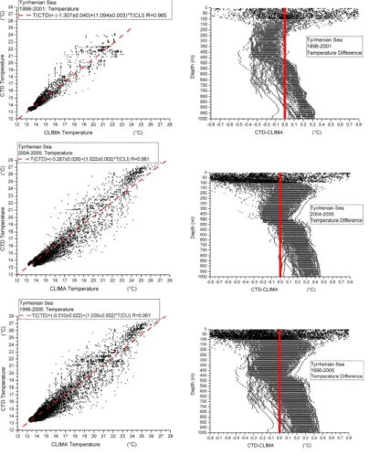
measurements, and gives a quantitative parameter of the possible evolution of water characteristics. Results concerning dataset 1996–2001 are plotted in Figs. 1a and b, whereas in Figs. 1c and d, and in Figs. 1e and f dataset 2004–2005 and dataset 1996– 2005, respectively, are shown. The fits of T measurements have the same relatively good quality, but the slope of 2004–2005 dataset indicates a deviation from

clima-10

tological values smaller than in the 1996–2001 one. In fact, when the temperature differences are analysed, the discrepancy between earlier and new measurements is evident. In 1996–2001 dataset, only cooler waters are present at depth ranging be-tween 200 and 500 m, whereas waters at deeper depth are warmer, up to +0.3◦C. In recent dataset, both warmer and cooler waters occur in the previous range of depth,

15

and a significant bump is evident below 500 m depth, with temperature differences within the range 0.1–0.4◦C.

As a further parameter to check the concordance between climatology and recent measurements, the correspondent σ values are analysed. In Fig. 2, the agreement between climatological and measured σ values, at depths ranging from 5 m down to

20

2350 m, is specified through the number of values differing less than the uncertainty used in this analysis. If recent values differ less than the allowed variability, such σ values can be thought as constant in time, and the temporal σ stability is verified. Such an assumption is reasonable (at a level of about 80%) down to 100 m depth in both datasets (Fig. 2a and b), mainly thanks to the large admitted variability. At deeper

25

depths, the stability is a robust hypothesis always verified, but the region between 100 and 1000-m depth puts in evidence significant differences, being the agreement at a level of 45% in the whole dataset (Fig. 2e), with a slightly better concordance

(13)

OSD

Full Screen / Esc

of values in more recent dataset. In general, recent measurements show that the water in Tyrrhenian Sea is generally warmer, saltier, and slightly denser than quoted by climatological datasets.

4 Synthetic salinity

The basic assumption of the proposed method is that in each sea region the local θ-S

5

relationship (as deduced from climatological dataset), and the accompanying σ profile evolve at seasonal time scale, but they have not significant variations at inter-annual time scale. This means, for instance, that different profiles as measured in the same day, but in different years, have to be assumed as coincident if their difference at each depth is within the oscillation range (due to instrumental errors and daily variability).

10

Deviations are admitted, and can be recognised and reproduced only when a trend occurs: this requires a transient phenomenon over a significant time interval (at least, more than one year).

The results detailed in Figs. 2a, b, and e indicate that the assumption of σ stability seems to be ruled out mainly at depths ranging from 100 down to 1000 m.

15

4.1 Proposed technique

Climatological T and S values, as deduced from monthly datasets, represent an aver-age based on a set of data and cannot describe a specific measurement. Therefore, a significant discrepancy between climatological values and real data can occur and, consequently, assimilation of salinity in models can show relevant disagreement and

20

uncertainty. In order to reduce such a discrepancy, modified salinity profiles (S_CLI∗ ) have been computed starting from climatological SCLIprofiles.

It has been supposed that a synthetic salinity profile (S_CLI∗ ) in a specific area can be computed starting from the correspondent climatological profile by introducing a cor-rection factor (CF) deduced from latest measurements in that region, and describing

(14)

OSD

Full Screen / Esc

EGU the difference averaged over time and space. The correction factor is a function fS

depending on measured temperature TX(h), climatological temperature TCLI(h), and

difference ∆T (h)=TX(h)−TCLI(h) between climatology and measurements. In short,

S_SYN∗ _(h)=S_CLI(h)·fS(h, TCLI(h), ∆T (h)), where the function fS will be shortly called CF

in the paper. The function calculates the ratio between all measured and

clima-5

tological values of salinity at each selected depth, climatological temperature, and temperature difference with respect to the climatology. The used range of variability is 12.0◦C≤T_CLI≤27.6◦C (step 0.2◦C) for temperature, and −4.0◦C≤∆T ≤+4.0◦C (step 0.1◦C, a value as great as the nominal sensitivity of XBT probes) for temperature dif-ference.

10

More in detail, each synthetic salinity profile is computed as follows:

1. σ profile is calculated from climatological T and S dataset and from the recent datasets, and its inversion are removed, if necessary;

2. Minimum (and maximum) of salinity and σ diminished (increased) by 0.01 units at each depth within a selected temperature interval is calculated from datasets of

15

recent measurements;

3. The maximum S and σ difference between the values measured at two consec-utive depths within the same temperature interval is calculated from recent mea-surements and increased by 0.01 units.

4. The basis of isothermal waters in upper region (usually in late summer, autumn

20

and winter) is determined by software, then the points 2 and 3 are repeated for this part of the profile.

5. SCLIprofile is multiplied by CF, and two conditions are imposed:

– the difference between the S values at two consecutive depths has to be not

greater than the maximum measured at a fixed depth and temperature;

(15)

OSD

Full Screen / Esc

– the S value at each depth has to be not greater (lower) than the maximum

(minimum) measured at a fixed depth and temperature;

6. A σ profile is computed by using such a modified S profile, and the same condi-tions as at point 5, but for potential density, are applied, also taking into account the occurrence of isothermal profiles. In such a case, σ inversions are eliminated,

5

and the profile is monotonically ordered. This is the “synthetic potential density profiles σ_SYN∗ (h)”.

7. From σ_SYN∗ (h), the salinity profile is computed, and conditions detailed at point 5 are newly applied. This is the “synthetic salinity profile S_SYN∗ (h)”.

4.2 Method validation

10

In order to check the validity of the proposed technique, the available time ordered dataset of profiles from Tyrrhenian Sea has been divided in sub-samples, and the cor-rection factor has been computed for each subset. Then, synthetic profiles have been obtained by using either the specific CF correspondent to the selected sub-sample or CF deduced from the remaining sub-sample. The comparison has been based on

15

the analysis of the correlation when synthetic values are plotted vs. climatology and measured values, and on the values of averaged differences.

An important step of the proposed method is the capability of reproduction of mea-sured values when CF is not deduced from the analysed dataset. Two are the selected computational ways to verify such a hypothesis, implying the use of CF deduced from

20

a dataset different in time, or from contemporaneous, but independent measurements. For the former, two interpretations are possible, depending on the capability the CF has to allow a right reproduction of measured values. An uncorrected description can be due either to the incapability of the method, or to a peculiar time evolution of physical parameters. In any case, the robustness of the dataset originating CF in order to have

25

(16)

OSD

Full Screen / Esc

EGU has been analysed in the same way as the Tyrrhenian one. Results of comparison with

such datasets are shortly detailed. 4.2.1 Tyrrhenian Sea

The proposed technique has been checked on time-ordered Tyrrhenian Sea 1996– 2005 dataset, and its sub-samples 1996–2001, 2004–2005, and 2004–2005 ODD and

5

2004–2005 EVEN. The latest datasets were created by extracting from 2004–2005 dataset profiles in position odd or even, respectively.

The analysis of sub-samples 1996–2001 and 2004–2005 highlights some details of the evolution of Tyrrhenian Sea water characteristics. The former confirms the differ-ences with respect to climatological values as evidenced by T profiles (Fig. 1b). Clearly,

10

Tyrrhenian waters are saltier at about 150 m depth (Fig. 3c) and below about 400 m depth (Fig. 3e), and σ values slightly increased (Figs. 3d and f). In this case, synthetic values give a better reproduction of measurements, but the agreement is poor for both

S and σ in the region between 100 and 400 m depth. Consequently, only 67% of σ_SYN∗ values in the region 100–1000 m agree with measurements. This could be due to the

15

rough and poor temporal and spatial coverage of the data and makes the CF values at those depths unstable and not sufficiently robust.

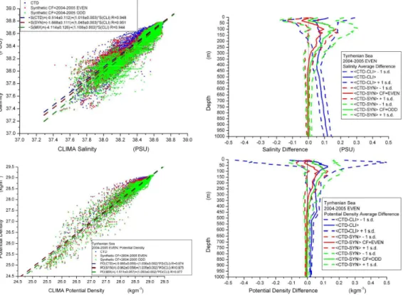
The analyses on 2004–2005 dataset reveal a different behaviour. The differences in temperature are lower (Fig. 1c), but a significant bump occurs below about 500 m depth (Fig. 1d), and salinity difference confirms such a variation (Fig. 4e). The capability of

20

synthetic values in reproducing real measurements is evident for both S and σ. The profile of salinity average difference (Figs. 4c and e) underlines a reduced discrepancy in the region between 100 and 300 m depth, mainly due to the influence of 2004 mea-surements. Similar conclusions are valid for potential density difference (Figs. 4d and f), where the agreement of fit coefficients is very good.

25

The results of the use in calculation of CFs extracted from a different dataset are explained in Figs. 2a and b, and Figs. 3 and 4 (green lines). The values of fit coefficients are acceptable for both the physical parameters, and improve the results based on

(17)

OSD

Full Screen / Esc

climatology. The correlation values indicate a sometimes-significant dispersion in both cases, 1996–2001 dataset with 2004–2005 CF, and 2004–2005 dataset with 1996– 2001 CF.

If CFs computed by sorting time-ordered and randomly distributed measurements are applied, interesting results occur. Climatological, synthetic and synthetic with

5

mixed CF plots vs. measurements of salinity for 2004–2005 EVEN dataset are shown in Figs. 5a and b, and in Figs. 6a and b for 2004–2005 ODD dataset. The values of the fit coefficients are in substantial agreement when synthetic salinity mixed results are compared, and well improve the climatology, but the correlation indicates a dispersion of synthetic values bigger than the occurrence when the proper CF is used. The σ

10

values computed with synthetic mixed CF are worse than the ones computed with their specific CF, but much better than the ones deduced from climatology (see Figs. 2c and d, and Figs. 5c and 6c).

The 1996–2005 dataset shows significant discrepancies from climatology in T , salin-ity and potential denssalin-ity values with interesting depth dependent differences. The fit

15

coefficients and correlation values of Fig. 7a indicate that Tyrrhenian waters are dif-ferent from climatological waters, with some evident changes in the region between 100 and 1000 m depth (Fig. 2e). In addition, the profile of salinity average difference displays an evident increased salinity value below about 400 m depth with respect to the climatology (Figs. 7c and e); σ values are also greater (Figs. 7d and f). When

20

S_SYN∗ and σ_SYN∗ values are considered, the difference with respect to measured val-ues is strongly reduced, and the strength and the depth dependence of the average difference (Figs. 7c and e for salinity, and Figs. 7d and f for potential density).

The analysis on Tyrrhenian datasets indicate that the proposed technique (comput-ing synthetic values for both S and σ start(comput-ing from T profiles, monthly climatological

25

datasets, and correction factor deduced from recent measurements), greatly improves the climatology, and has usually a good agreement with real data. As a marginal re-sult, in order to obtain a robust CF it is fundamental to have a dataset homogeneous in space and time or, at least, with a good seasonal sampling.

(18)

OSD

Full Screen / Esc

EGU 4.2.2 Ligurian Sea

The strong discrepancy between climatology and measurements in Ligurian Sea datasets is evident in plots concerning 1996–2005 dataset (see Fig. 8a for temper-ature, c for salinity, and e for potential density), as well as the bad quality of the related fits. Recent measurements and climatology disagree, both for S (Figs. 8c and d), and

5

σ_{(Figs. 8e and f). Bad values of fit coefficients for both S and σ and of the correlation}

clearly confirm the visual results (Figs. 8c and e).

In addition, 2004–2005 measurements indicate discrepancies of different kind with respect to the previous ones, and significantly saltier and denser waters appear in region down to 300 m depth (see Fig. 9a for temperature, c and d for salinity, and e

10

and f for potential density). The values of fit coefficients and of the agreement between measurements and σ_CLI values (Figs. 9c and e) indicate the occurrence of relevant physical phenomena in such a region.

5 Comparison with XCTD measurements

Synthetic values of salinity (and potential density) have been compared with profiles

15

obtained in Tyrrhenian Sea by using 21 Sippican XCTD-1 Digital probes (manufac-tured by TSK, Yokohama – Japan) dropped in May, September and October 2004. Such expandable instruments have improved uncertainty in temperature values when compared to XBT probes (δT ∼0.01◦C instead of δT ∼0.10◦C), whereas the uncertainty on S is about 0.03 PSU. Climatological and measured values are compared with

syn-20

thetic values as computed by using Tyrrhenian 2004–2005 dataset and the related CF, and the results are shown in Fig. 10. Despite the small available sample, T values are in general greater than climatology states (Fig. 10b), even if the fit does not display strong disagreement (Fig. 10a). Similar behaviour occurs when salinity is analysed: the fit coefficients show that saltier values occur mainly below 200 m depth, but the

25

(19)

repro-OSD

Full Screen / Esc

duce measured values better than climatology, but a disagreement remains (Fig. 10d). Synthetic values overestimate real measurements, even if the disagreement is more or less constant below 200 m depth, at a level of about 0.05 PSU. The results of analy-ses on potential density are similar (Fig. 10e), even if σ_SYN∗ well fits the measurements (Fig. 10f): in fact, σ_SYN∗ values overestimate measurements, but the difference is

prac-5

tically constant below 200 m depth, at a level of about 0.03 kgm−3.

6 Application to XBT profiles

The proposed technique has been applied to T profiles obtained from XBT probes dropped along the transect Genova-Palermo, from May 2004 to December 2005, dur-ing 15 monthly cruises, with the exception of June, July and August 2004, and of July

10

and August 2005. The sample consists of 414 profiles from Tyrrhenian Sea and of 119 profiles from Ligurian Sea, the maximum depth being 890 m and 770 m, respectively. The advantage in having such repeated measurements done by VOS activity is just the possibility to study the time evolution of water characteristics, but only T values are recorded by XBT probes, a similar monitoring activity being much more expensive

15

when XCTD probes are dropped.

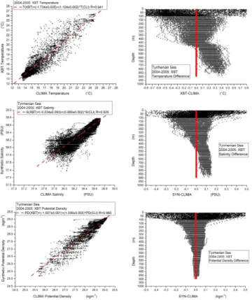
The measured T values have a not negligible difference with respect to the climato-logical values (Fig. 11a), and all the measurements at depth deeper than 500 m indi-cate values warmer than before, within the range of 0.1–0.4◦C (Fig. 11b). The corre-sponding CTD sample has a lower difference, but the sampled area is slightly different.

20

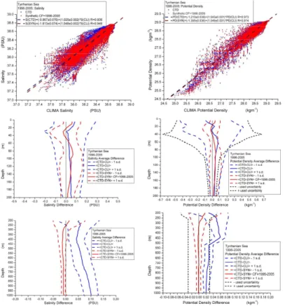
When S_SYN∗ and σ_SYN∗ are compared with results obtained by using Tyrrhenian 2004– 2005 dataset, a general concordance appears. More in detail, salinity shows larger discrepancy (Fig. 11c and d vs. Figs. 4c and d) than potential density has (Figs. 11e and f vs. Figs. 4e and f), both in fit coefficients and average differences. This could be partially attributed to the characteristics of available sample of CTD casts, which is

25

highly inhomogeneous in time and in space, with respect to the XBT dataset, which includes T profiles monthly recorded on the same transect.

(20)

OSD

Full Screen / Esc

EGU The comparison of XBT profiles in Ligurian Sea with climatological T profiles shows

a not negligible difference (Fig. 12a), even if the quality of the fit is good. Unfortunately, few profiles have depth deeper than 550 m (Fig. 12b), but the available data put in evidence a clear seawater warming process, less evident in near surface layers. When

S_SYN∗ _{profiles are analysed, a significant difference appears in the fit, which has a rough}

5

quality (Fig. 12c), but results shown in Fig. 9c are confirmed. The difference profiles (Fig. 12d) also confirms the previous results on Ligurian Sea (Fig. 9d). Analyses on

σ_SYN∗ profiles indicate that the fit seems to be acceptable, but not excellent (Fig. 12e). More in detail, slightly lower σ values occur in the region between about 200 and 400 m depth, whereas there is a small increment at deeper depth (Fig. 12f).

10

7 Discussion and conclusion

Very recently, the need of contemporaneous and co-located T and S profiles has in-creased significantly in ocean forecasting, due to the multivariate data assimilation schemes, which are still in progress. In general, models assimilate satellite data (sea surface temperature and height), and T profiles (e.g. Pinardi et al., 2002), whereas

15

S values are measured only by Argo, GLIDER and CTD (or XCTD). Because of the large difference between the cost of T and S profiles, T measurements are much more than S profiles. In addition, the confidence in salinity climatological dataset is lower than in the temperature dataset. In any case, S profiles are usually “extracted” from climatological datasets, even if the applied technique is quite different (i.e. De Mey and

20

Benkiran, 2002; Fox et al., 2002; Thacker, 2006).

MEDATLAS/MED6 climatological monthly dataset is a reference dataset for Mediter-ranean Sea, but it does not reproduce local and peculiar situations, and the derived σ profiles (even if an oscillation band, due to the addition of daily variation and instrumen-tal uncertainty, is added), indicate a significant difference from recent measurements.

25

When a day-by-day linear evolution during a month is applied to the seawater σ values, the improvements are negligible.

(21)

OSD

Full Screen / Esc

In general, synthetic values computed by applying the technique proposed in this pa-per have a good agreement with measured S and σ values: the fit coefficients and the correlation confirm it. The proposed correction factor seems to be able to describe the main part of the difference that recent measurements in Tyrrhenian and Ligurian Seas show with respect to the climatological values. The addition of other recent T and S

5

profiles, assuring a more homogeneous temporal and geographic coverage, improves the stability and the robustness of the correction factor. In this case, σ_SYN∗ and S_SYN∗ profiles should have a further reduced discrepancy with respect to the experimental data. Analyses on Tyrrhenian and Ligurian Seas seem to indicate that measurements seasonally repeated can check the variability of water characteristics, and allow the

10

computation of a sufficiently robust correction factor.

A significant check of the validity and robustness of S values obtained by apply-ing this method could be done by comparapply-ing dynamical height values with sea level anomalies and heights as deduced from satellite measurements. In this case, the tran-sect Genova-Palermo is nearly coincident with the pass number 44 of the JASON-1

15

satellite. Aiming to this further but significant control, all the cruises along that transect were made within 24 h from the passage of satellite, in order to minimize the possible difference of sea conditions.

The major problem discussed in this paper is the implementation of a methodology capable to estimate S from climatological data. The proposed method is based on the

20

θ-S relationship and the stability of water properties: it allows the estimate of S and

σfrom T profiles with the addition of few phenomenological constraints. The obtained results are in general good agreement with measurements.

The most significant deviations can occur in regions of particular vertical movements: in such cases, the θ-S characteristics do not respect the basic hypothesis of relatively

25

small mixing. It must be underlined that even other methods based on EOF tech-nique require a basic long-term stability, but the reconstruction of salinity remains a not completely solved problem, that must be addressed to provide “good” data for multi-parametric data assimilation.

(22)

OSD

Full Screen / Esc

EGU It has to be pointed out that one of the properties of this technique is the rapidity in

calculation. If datasets for climatology and for the computation of the correction factor are available, some minutes are required to calculate S_SYN∗ and σ_SYN∗ profiles from a set of XBT profiles. Therefore, in this case it should be possible to release at the same time quality checked XBT T profiles with estimated S and σ associated profiles.

5

Acknowledgements. The author acknowledges the contribution of scientists and technicians

participating to MFS-PP and MFS-TEP projects, and of M. Astraldi (CNR-ISMAR, Lerici-Italia), who made available CTD data collected in Tyrrhenian and Ligurian Seas. Many thanks to G. Manzella (ENEA, Lerici-Italia) for suggestions and criticisms during the preparation of this paper. This work is supported by the European Commission (MAST contract

MAS3-CT98-10

0171), and Italian Ministry of Research (contract “Ambiente Mediterraneo”).

References

Bleck, R.: An oceanic general circulation model framed in hybrid isopycnic-Cartesian coordi-nates, Ocean Modelling, 37, 55–88, 2002.

Brankart, J. M. and Pinardi, N.: Abrupt cooling of the Mediterranean Levantine Intermediate

15

Water at the beginning of the 1980s: observational evidence and model simulation, J. Phys. Oceanogr., 31, 2307–2320, 2001.

Brasseur, P., Beckers, J. M., Brankart, J. M., and Schoenauen, R.: Seasonal Temperature and Salinity fields in the Mediterranean Sea: Climatological analyses of an historical data set, Deep-Sea Res., 43(2), 159–192, 1996.

20

Carnes, M. R., Teague, W. J., and Mitchell, J. L.: Interference of subsurface structure from field measurable by satellite, J. Atmos. Oceanic Technol., 11, 551–566, 1994.

De Mey, P. and Benkiran, M.: A multivariate reduced-order optimal interpolation method and its application to the Mediterranean basin-scale circulation, in: Ocean Forecasting, edited by: Pinardi, N. and Woods, J., Springer Verlag, 281–306, 2002.

25

Demirov, E., Pinardi, N., De Mey, P., Tonani, M., and Fratianni, C.: Assimilation scheme of the Mediterranean Forecasting System: Operational implementation, Ann. Geophys., 21, 189–203, 2003,http://www.ann-geophys.net/21/189/2003/.

(23)

OSD

Full Screen / Esc

Donguy, J. R.: Surface and subsurface Salinity in the tropical Pacific Ocean. Relations with climate, Progress in Oceanography, 34, 45–78, 1994.

Donguy, J. R., Eldin, G., and Wyrtki, K.: Sealevel and dynamic topography in the western Pacific during 1982-1983 El Nino, Tropical Ocean-Atmospheric Newsletters, 36, 1–3, 1986. Emery, W. J.: Dynamic height from Temperature profiles, J. Phys. Oceanogr., 5, 369–375,

5

1975.

Emery, W. J. and Dewar, J. S.: Mean salinity, salinity-depth and Temperature-depth curves in the North Atlantic and North Pacific, Progress in Oceanography, 11, 219– 305, 1982.

Emery, W. J. and O’Brien, A.: Inferring Salinity from Temperature or depth for dynamic height

10

calculations in the North Pacific, Atmosphere-Ocean, 16, 348–366, 1978.

Emery, W. J. and Wert, R. T.: Temperature-Salinity curves in the Pacific and their application to dynamic height computation, Journal of Physical Oceanography, 6, 613–617, 1976.

Fox, D. N., Teague, W. J., Barron, C. N., Carnes, M. R., and Lee, C. M.: The modular ocean data assimilation system (MODAS), Journal of Atmospheric and Oceanic Technologies, 19,

15

240–252.

Fusco, G., Manzella, G. M. R., Cruzado, A., Gacic, M., Gasparini, G. P., Kovacevic, V., Millot, C., Tziavos, C., Velasquez, Z. R., Walne, A., Zervakis, V., and Zodiatis, G.: Variability of mesoscale features in the Mediterranean Sea from XBT data analysis, Ann. Geophys., 21, 1–12, 2003,http://www.ann-geophys.net/21/1/2003/.

20

Haines, K., Blower, J., Drecourt, J., Liu, C., Vidard, A., Astin, I., and Zhou, X.: Salinity assim-ilation using S(T) relationship: Covariance Relationships, Monthly Weather Review, 134(3), 759–771, 2006.

Halliwell Jr., G. R.: Evaluation of vertical coordinate and vertical mixing algorithms in the hybrid-coordinate ocean model HYCOM, Ocean Modelling, 7, 285–322, 2005.

25

Hansen, D. V. and Thacker, W. C.: Estimation of Salinity profiles in the upper ocean, J. Geophys. Res., 104(4), 7921–7933, 1999.

K ¨ase, R. H., Hinrichsen, H. H., and Sanford, T. B.: Inferring density from temperature via density-ratio relation, J. Atmos. Oceanic Technol., 13, 1202–1208, 1996.

Kessler, W. S. and Taft, B. A.: Dynamics heights and zonal geostrophic transports in the central

30

tropical Pacific during 1979–1984, J. Phys. Oceanogr., 17, 97–122, 1987.

Lagerloef, G. S. E.: An alternate method for estimating dynamic height from XBT profiles using empirical vertical modes, J. Phys. Oceanogr., 24, 205–213, 1994.

(24)

OSD

Full Screen / Esc

EGU

Maes, C.: A note on the vertical scales of Temperature and Salinity and their signature in dynamic height in the western Pacific Ocean, J. Geophys. Res., 104(5), 11 037–11 048, 1999.

Maes, C. and Behringer, D. W.: Using satellite-derived sea level and Temperature profiles for determining the Salinity variability: a new approach, J. Geophys. Res., 105(4), 8537–8547,

5

2000.

Maes, C., Behringer, D. W., and Reynolds, R. W.: Retrospective analysis of the Salinity vari-ability in the western tropical Pacific Ocean using an indirect minimization approach, Journal of Atmospheric and Oceanic Technology, 17, 512–524, 2000.

Maillard, C. and Fichant, M.: MEDAR-MEDATLAS Protocol. Part I. Exchange format and quality

10

checks for observed profiles, Rap. Int. TMSI/IDM/SISMER/SIS00-084, 2001.

Manzella, G. M. R., Cardin, V., Cruzado, A., Fusco, G., Gacic, M., Galli, C., Gasparini, G. P., Gervais, T., Kovacevic, V., Millot, C., Petit de la Villeon, L., Spaggiari, G., Tonani, M., Tziavos, C., Velasquez, Z., Walne, A., Zervakis, V., and Zodiatis, G.: EU-sponsored effort improves monitoring of circulation variability in the Mediterranean, Transactions, American

15

Geophysical Union, 82(43), 497–504, 2001.

Manzella, G. M. R. (MFS-VOS Group): A Marine Information System for Ocean Predictions, in: Ocean Forecasting: Conceptual Basis and Applications, edited by: Pinardi, N. and Woods, J. D., Springer-Verlag, Heidelberg, 37–53, 2002.

Manzella, G. M. R., Scoccimarro, E., Pinardi, N., and Tonani, M.: Improved near real time

20

data management procedures for the Mediterranean ocean Forecasting System – Voluntary Observing Ship Program, Ann. Geophys., 21, 49–62, 2003,

http://www.ann-geophys.net/21/49/2003/.

Medar Group: MEDAR/MEDATLAS Protocol (Version 3): Part I: Exchange Format and Quality Checks for Observed Profiles, Rap. Int. IFREMER/TMSI/IDM/SIS002-006, 2001.

25

Medatlas Group: Specifications for Mediterranean data banking and regional quality controls, IFREMER, Direction Scientifique, Sismer-Brest, SISMER/IS/94-014, 1994.

Pinardi, N., Allen, I., Demirov, E., De Mey, P., Korres, G., Lascaratos, A., Le Traon, P. Y., Maillard, C., Manzella, G. M. R., and Tziavos, C.: The Mediterranean Ocean forecasting system: first phase of implementation (1998–2001), Ann. Geophys., 21, 3–20, 2003,

30

Pinardi, N., Auclair, F., Cesarini, C., Demirov, E., Fonda Umani, S., Giani, M., Montanari, G., Oddo, P., Tonani, M., and Zavatarelli, M.: Toward marine environmental prediction in the

(25)

OSD

Full Screen / Esc

Mediterranean Sea coastal areas: a monitoring approach, in: Ocean Forecasting: Con-ceptual Basis and Applications, edited by: Pinardi, N. and Woods, J. D., Springer-Verlag, Heidelberg, 339–376, 2002.

Schmitt, R. W.: Form of the Temperature-Salinity relationship in the Central Water: evidence for double-diffusive mixing, J. Phys. Oceanogr., 11, 1015–1026, 1981.

5

Siedler, G. and Stramma, L.: The applicability of the T/S method to geopotential anomaly computations in the North Atlantic, Oceanologica Acta, 6(2), 167–172, 1982.

Sparnocchia, S., Pinardi, N., and Demirov, E.: Multivariate empirical orthogonal function anal-ysis of the upper thermocline structure of the Mediterranean Sea from observations and model simulations, Ann. Geophys., 21, 167–187, 2003,

10

Stommel, H. S.: Note on the use of the T-S correlation for dynamic height anomaly calculations, J. Mar. Res., 2, 85–92, 1947.

Sverdrup, H. V., Johnson, M. W., and Fleming, R. H.: The Ocean: Their Physics, Chemistry and general Biology, Prentice Hall, 1087, 1942.

15

Thacker, W. C. and Esenkov, O. E.: Assimilating XBT data into HYCOM, J. Atmos. Oceanic Technol., 19, 709–724, 2002.

Thacker, W. C.: Estimating salinity to complement observed temperature: 1 – Gulf of Mexico, J. Mar. Syst., in press, 2006.

Thacker, W. C. and Sindlinger, L.: Estimating salinity to complement observed temperature:

2-20

Northwest Atlantic, Journal of Marine System, in press, 2006.

Troccoli, A. and Haines, K.: Use of temperature-salinity relation in a data assimilation context, Journal of Atmospheric and Oceanic Technology, 16, 2011–2025, 1999.

Vignudelli, S., Cipollini, P., Reseghetti, F., Fusco, G., Gasperini, G. P., and Manzella, G. M. R.: Comparison between XBT data and TOPEX/Poseidon

satel-25

lite altimetry in the Ligurian-Tyrrhenian area, Ann. Geophys., 21, 123–135, 2003, http://www.ann-geophys.net/21/123/2003/.

Vossepoel, F. C., Reynolds, R. W., and Miller, L.: Use of sea level observations to estimate Salinity variability in the tropical Pacific, J. Atmos. Oceanic Technol., 16, 1401–1415, 1999. Woodgate, R. A.: Can we assimilate temperature data alone into a full equation of state model?,

30

Ocean Modelling, 114, 4–5, 1997.

W ¨ust, G.: On the vertical circulation of the Mediterranean Sea, J. Geophys. Res., 66(10), 3261–3271, 1961.

(26)

OSD

Full Screen / Esc

EGU Table 1. Temporal distribution of profiles from Tyrrhenian Sea.

Year Jan Feb March April May June July Aug Sep Oct Nov Dec Total

1996 – – – 4 4 24 – – 17 – – – 49 1997 16 – – – – – – – – 19 5 – 40 1998 – – – – 15 – – – – – – – 15 1999 – – – – – – – – – – – 8 8 2001 2 – – – – – – – – 5 – – 7 2004 24 – – – 34 – – 90 14 16 12 7 197 2005 6 3 9 13 45 9 6 8 9 7 5 5 125 Total 48 3 9 17 98 33 6 98 40 47 22 20 441

(27)

OSD

Full Screen / Esc

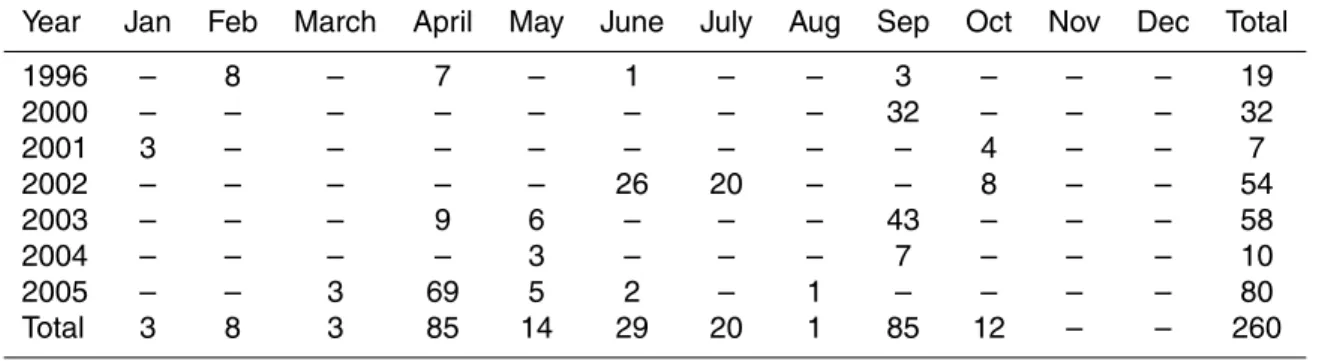
Table 2. Temporal distribution of profiles from Ligurian Sea.

Year Jan Feb March April May June July Aug Sep Oct Nov Dec Total

1996 – 8 – 7 – 1 – – 3 – – – 19 2000 – – – – – – – – 32 – – – 32 2001 3 – – – – – – – – 4 – – 7 2002 – – – – – 26 20 – – 8 – – 54 2003 – – – 9 6 – – – 43 – – – 58 2004 – – – – 3 – – – 7 – – – 10 2005 – – 3 69 5 2 – 1 – – – – 80 Total 3 8 3 85 14 29 20 1 85 12 – – 260

(28)

OSD

Full Screen / Esc

EGU Table 3. Influence of uncertainties of temperature and salinity on potential density (σ) (the

values are in kgm−3).

δT = ±0.01◦

C δT = ±0.10◦

C δS = ±0.01 PSU δS = ±0.01 PSU δS = ±0.01 PSU δT = ±0.01◦C _{δT = ±0.10}◦

C 0–100 m δσ = ±0.0026 δσ = ±0.0265 δσ = ±0.0078 δσ = ±0.0065 δσ = ±0.0337 >100 m δσ = ±0.0021 δσ = ±0.0208 δσ = ±0.0078 δσ = ±0.0065 δσ = ±0.0290

(29)

OSD

Full Screen / Esc

Fig. 1. Climatological vs. measured temperatures from Tyrrhenian Sea for different datasets, on

left column, and the differences of temperature between CTD measurements and climatology, right column. In order to enhance the differences, only values down to 1000 m depth have been

(30)

OSD

Full Screen / Esc

EGU Fig. 2. The robustness of potential density stability hypothesis for the Tyrrhenian Sea, at depths

ranging from 5 m down to 2350 m, is verified through the evaluation of the number of climatolog-ical and synthetic values having a difference, with respect to the measured ones, smaller than the uncertainty used in the analysis. The percent ratio between the number of climatological (or synthetic) values satisfying the request and the measured values is plotted. If such a case occurs, the values are undistinguishable: consequently, the physical properties of water should be not significantly changed (constancy in time). Synthetic Mixed values are computed by us-ing CF from a different dataset. The depth interval has been shared as follows: Top (0–100 m), Intermediate (100–1000 m), and Bottom (1000–2350 m).

(31)

OSD

Full Screen / Esc

Fig. 3. Comparison among climatology, measured and synthetic values of salinity (left column)

and potential density (right column) for Tyrrhenian 1996–2001 dataset. The average differences are also plotted. Synthetic values have been computed both by using the specific CF (red), and from other dataset (green). Synthetic values offer a better description of measurements, mainly at depth deeper than 400 m: fit coefficients give a confirmation of such an improvement. For potential density, the uncertainty values used in calculations are shown.

(32)

OSD

Full Screen / Esc

EGU Fig. 4. The same as in Fig. 3, but for Tyrrhenian 2004–2005 dataset, which will be the basis of

correction factor for the analyses on XBT data. The good agreement between CTD measure-ments and synthetic S and σ values is evident.

(33)

OSD

Full Screen / Esc

Fig. 5. Salinity and potential density results for Tyrrhenian 2004–2005 EVEN dataset. Here and

in Fig. 6, results of analyses with correction factors from independent, but contemporaneous and co-located measurements are detailed. The obtained results well improve the climatolog-ical dataset, even if an unexpected significant difference occurs at depth lower than 300 m for salinity and potential density.

(34)

OSD

Full Screen / Esc

EGU Fig. 6. The same as in Fig. 5, but for Tyrrhenian 2004–2005 ODD dataset. The results are

(35)

OSD

Full Screen / Esc

Fig. 7. The same as in Fig. 3, but for Tyrrhenian 1996–2005 dataset, the full available sample.

Because of a larger (both geographically and temporarily speaking) dataset, the correction factor includes a more complete set of physical states, allowing the synthetic values to give a more precise reproduction of real seawater characteristics.

(36)

OSD

Full Screen / Esc

EGU Fig. 8. The plots describing the main results on Ligurian 1996–2005 dataset are shown. CTD

temperature values have a well identifiable difference from climatological dataset. Both salinity and potential density synthetic values well reproduce CTD measurements, and put in evidence a different behaviour with respect to the climatology.

(37)

OSD

Full Screen / Esc

Fig. 9. The same as in Fig. 8, but for Ligurian 2002–2005 dataset, which will be used in

analyses on XBT from Ligurian Sea. Similar conclusions with respect to the whole 1996–2005 are possible, mainly for the bad quality of the fit of S values.

(38)

OSD

Full Screen / Esc

EGU Fig. 10. Main results of analyses on 2004 XCTD dataset (21 profiles) from Tyrrhenian Sea.

Almost all the probes were dropped in May and September 2004, the used correction factor is from 2004–2005 dataset. This could explain some small differences, mainly in S values, between synthetic and XCTD measurements. The systematic overestimate that S∗

SYNand σ ∗ SYN

(39)

OSD

Full Screen / Esc

Fig. 11. Main results of analyses on Tyrrhenian 2004–2005 XBT dataset. A comparison can be

done with Figs. 1c and d for temperature and Fig. 4 for salinity and potential density plots. The temperature difference has similar behaviour, but the fit puts in evidence a stronger increment in XBT temperature values than in CTD measured, even with different sampling strategy (the same repeated transect for XBT dataset and “random strategy” for CTD dataset). Salinity values indicate a complicate variability down to about 400 m depth, and a well evident increment at deeper depth is strongly confirmed. On the other hand, σ values show a better global

(40)

OSD

Full Screen / Esc

EGU Fig. 12. The same as in Fig. 11, but for Ligurian 2004–2005 XBT dataset. In this case, results

have to be compared with Fig. 9. It has to be remarked the difference in available depth between the dataset and the different sampling strategy (the same repeated transect for XBT dataset and “random strategy” for CTD dataset). A substantial agreement in temperature fit appears, whereas S values show a different behaviour both in the fit and in the difference plot down to 350 m depth. On the other hand, σ values have a smaller discrepancy.