HAL Id: hal-00296440
https://hal.archives-ouvertes.fr/hal-00296440
Submitted on 12 Feb 2008
HAL is a multi-disciplinary open access
archive for the deposit and dissemination of
sci-entific research documents, whether they are
pub-lished or not. The documents may come from
teaching and research institutions in France or
abroad, or from public or private research centers.
L’archive ouverte pluridisciplinaire HAL, est
destinée au dépôt et à la diffusion de documents
scientifiques de niveau recherche, publiés ou non,
émanant des établissements d’enseignement et de
recherche français ou étrangers, des laboratoires
publics ou privés.
MIPAS SF6 measurements
G. P. Stiller, T. von Clarmann, M. Höpfner, N. Glatthor, U. Grabowski, S.
Kellmann, A. Kleinert, A. Linden, M. Milz, T. Reddmann, et al.
To cite this version:
G. P. Stiller, T. von Clarmann, M. Höpfner, N. Glatthor, U. Grabowski, et al.. Global distribution of
mean age of stratospheric air from MIPAS SF6 measurements. Atmospheric Chemistry and Physics,
European Geosciences Union, 2008, 8 (3), pp.677-695. �hal-00296440�
www.atmos-chem-phys.net/8/677/2008/
© Author(s) 2008. This work is distributed under the Creative Commons Attribution 3.0 License.
Chemistry
and Physics
Global distribution of mean age of stratospheric air from MIPAS
SF
6
measurements
G. P. Stiller1, T. von Clarmann1, M. H¨opfner1, N. Glatthor1, U. Grabowski1, S. Kellmann1, A. Kleinert1, A. Linden1, M. Milz1,*, T. Reddmann1, T. Steck1, H. Fischer1, B. Funke2, M. L´opez-Puertas2, and A. Engel3
1Forschungszentrum Karlsruhe and University of Karlsruhe, Inst. f¨ur Meteorologie und Klimaforschung, Karlsruhe, Germany 2Instituto de Astrof´ısica de Andaluc´ıa CSIC, Granada, Spain
3Institut f¨ur Atmosph¨are und Umwelt, J.W. Goethe Universit¨at Frankfurt am Main, Frankfurt, Germany *now at: Institutionen f¨or Rymdvetenskap, Lule˚a Tekniska Universitet, Kiruna, Sweden
Received: 27 July 2007 – Published in Atmos. Chem. Phys. Discuss.: 18 September 2007 Revised: 3 January 2008 – Accepted: 8 January 2008 – Published: 12 February 2008
Abstract. Global distributions of profiles of sulphur hexafluoride (SF6) have been retrieved from limb emission
spectra recorded by the Michelson Interferometer for Passive Atmospheric Sounding (MIPAS) on Envisat covering the pe-riod September 2002 to March 2004. Individual SF6
pro-files have a precision of 0.5 pptv below 25 km altitude and a vertical resolution of 4–6 km up to 35 km altitude. These data have been validated versus in situ observations obtained during balloon flights of a cryogenic whole-air sampler. For the tropical troposphere a trend of 0.230±0.008 pptv/yr has been derived from the MIPAS data, which is in excellent agreement with the trend from ground-based flask and in situ measurements from the National Oceanic and Atmospheric Administration Earth System Research Laboratory, Global Monitoring Division. For the data set currently available, based on at least three days of data per month, monthly 5◦ latitude mean values have a 1σ standard error of 1%. From the global SF6distributions, global daily and monthly
distri-butions of the apparent mean age of air are inferred by appli-cation of the tropical tropospheric trend derived from MIPAS data. The inferred mean ages are provided for the full globe up to 90◦N/S, and have a 1σ standard error of 0.25 yr. They range between 0 (near the tropical tropopause) and 7 years (except for situations of mesospheric intrusions) and agree well with earlier observations. The seasonal variation of the mean age of stratospheric air indicates episodes of severe in-trusion of mesospheric air during each Northern and South-ern polar winter observed, long-lasting remnants of old, sub-sided polar winter air over the spring and summer poles, and a rather short period of mixing with midlatitude air and/or
Correspondence to: G. P. Stiller ([email protected])
upward transport during fall in October/November (NH) and April/May (SH), respectively, with small latitudinal gradi-ents, immediately before the new polar vortex starts to form. The mean age distributions further confirm that SF6 is
de-stroyed in the mesosphere to a considerable degree. Model calculations with the Karlsruhe simulation model of the mid-dle atmosphere (KASIMA) chemical transport model agree well with observed global distributions of the mean age only if the SF6sink reactions in the mesosphere are included in
the model.
1 Introduction
According to model predictions, climate change is expected to intensify the Brewer-Dobson circulation (e.g. Buchart et al., 2006; Austin and Li, 2006). This would mean that stratospheric air will become younger within a global warm-ing scenario, providwarm-ing feedback to stratospheric chemistry, e.g. the chlorine load (Waugh et al., 2007; Waugh and Hall, 2002). A measure of the transport time of an air parcel trav-elling from the tropopause to a certain location in the strato-sphere is the so-called age of stratospheric air (Kida, 1983; Waugh and Hall, 2002). Due to mixing, an air parcel con-sists of air of different ages, characterized by its age spec-trum (Waugh and Hall, 2002). The average over the age distribution is known as the mean age of stratospheric air, Ŵ. Austin and Li (2006) have demonstrated that the mean age of stratospheric air is a suitable measure for the inten-sity of the Brewer-Dobson circulation or the upwelling flux. The mean age of air is lowest near the tropical tropopause and increases both with latitude and altitude (Waugh and Hall, 2002), reflecting the respective travelling times in the
global circulation. The mean age of stratospheric air can be derived from trace species which are stable within the troposphere and stratosphere and have a considerable trend which is, in the ideal case, linear. One suitable tracer for the measurement of the mean age of stratospheric air is sulphur hexafluoride (SF6). It is produced almost entirely
anthro-pogenically (Ko et al., 1993), has a well documented tropo-spheric increase and is chemically inert in the troposphere and stratosphere. The tropospheric increase has been linear for the last years and was consistent to a quadratic growth rate, with a very small quadratic term, however, before 1996 (Geller et al., 1997). The only sinks to be considered are photolysis and electron capture reactions in the mesosphere (Morris et al., 1995; Ravishankara et al., 1993; Reddmann et al., 2001) leading to atmospheric lifetimes of several hun-dreds to thousands of years (Ravishankara et al., 1993; Mor-ris et al., 1995). The mean age of air derived from SF6 is
generally in good agreement with that inferred from other tracers except in the polar vortices where intrusions of SF6
-depleted mesospheric air may play a role (Waugh and Hall, 2002). The mean age of air derived from SF6 and not
cor-rected for the mesospheric loss is sometimes referred to as the “apparent” mean age; whenever in this paper mean age of air derived from measured SF6is mentioned, the apparent
mean age is meant.
Measurements of SF6 and the mean age, in particular in
the stratosphere, have been rather sparse until now. Long-term surface in situ and flask measurements from numer-ous sites are provided by the National Oceanic and At-mospheric Administration (NOAA) Earth System Research Laboratory (ESRL), Global Monitoring Division (GMD) via ftp://ftp.cmdl.noaa.gov/hats/sf6/. An airborne data set mea-sured during various NASA ER-2 flights during the period 1992–1997 provided the most comprehensive stratospheric data set for Ŵ derived from CO2and SF6observations
cov-ering all latitudes between 85◦N and 60◦S, but only at one altitude (Boering et al., 1996; Elkins et al., 1996). Besides these observations, few vertical profiles from balloon-borne and airborne in situ and cryosampler instruments exist (An-drews et al., 2001; Strunk et al., 2000; Ray et al., 1999, 2002; Volk et al., 1997; Engel et al., 2006a,b). A few spectroscopic measurements of SF6 in the infrared have been performed
from the ground (Zander et al., 1991; Rinsland et al., 2003) and from the space-borne instruments ATMOS on the Space Shuttle (Rinsland et al., 1990; Zander et al., 1992; Rins-land et al., 1993) and ACE-FTS on SCISAT (RinsRins-land et al., 2005).
Recently Burgess et al. (2004, 2006) provided first global datasets of SF6 from Michelson Interferometer for
Pas-sive Atmospheric Sounding/Environmental satellite (MI-PAS/Envisat) spectral observations. They used MIPAS spec-tral data versions 4.53 to 4.59 (so-called “near-real time (NRT)” spectral data) for their analyses. The SF6 global
distributions revealed the main expected features, however, they were biased low by approximately 0.4 pptv compared to
the NOAA/ESRL/GMD surface flask measurements. To our knowledge, no attempt has been made to derive the mean age of stratospheric air from this data set so far.
In this paper, we present an alternative approach to re-trieve SF6from MIPAS/Envisat spectral data. Our data
anal-ysis is based on MIPAS high resolution spectra (ESA data version 4.61/62, so-called “re-processed” spectra) obtained from September 2002 to March 2004. After the descrip-tion of the retrieval approach and the data characterizadescrip-tion in terms of vertical resolution and error budget, global distribu-tions of SF6are presented. We validate individual profiles by
comparison to balloon-borne in situ observations. The trop-ical tropospheric yearly increase is derived and compared to NOAA/ESRL/GMD surface in situ and flask measurements. The trend derived from the MIPAS measurements in combi-nation with the long running NOAA/ESRL/GMD time series has been applied to infer the global distribution of mean age of stratospheric air, Ŵ. These data are compared to earlier observations, and their variation with time, altitude and lat-itude is analysed. Finally we address the importance of the mesospheric sink for age of air assessments from SF6.
2 MIPAS
The Michelson Interferometer for Passive Atmospheric Sounding (MIPAS) is a mid-infrared Fourier transform limb emission spectrometer designed and operated for measure-ment of atmospheric trace species (Fischer et al., 2007). Its spectral resolution in its original measurement mode was 0.035 cm−1, corresponding to an effective spectral
resolu-tion of 0.05 cm−1after numerical apodization with the
Nor-ton Beer “strong” apodization function (NorNor-ton and Beer, 1976). It operated in this mode from March 2002 to March 2004. MIPAS is operated on the Envisat polar orbiting satel-lite and records a rear-viewing limb sequence of 17 spectra each 90 s, corresponding to an along track sampling of ap-proximately 500 km and providing about 1000 vertical pro-files per day along 14 orbits in its original observation mode. The vertical tangent altitude spacing is 3 km between 6 km and 42 km, which is the altitude range relevant to this study. The raw signal is processed by the European Space Agency (ESA) to produce calibrated geolocated limb emission spec-tra, labelled level 1-B data (Nett et al., 1999). After an in-strument failure in March 2004, MIPAS resumed operation in a reduced spectral resolution mode with a variety of scan patterns providing different altitude coverage, horizontal and vertical sampling. For this study, level 1-B version 4.61/62 data (so-called “reprocessed” data) from September 2002 to March 2004 have been used.
3 SF6retrieval
3.1 Retrieval strategy
Retrievals presented here were carried out with the scientific MIPAS level 2 processor developed and operated by the In-stitute of Meteorology and Climate Research (IMK) in Karl-sruhe together with the Instituto de Astrof´ısica de Andaluc´ıa (IAA) in Granada. The general retrieval strategy, which is a constrained multi-parameter non-linear least squares fitting of measured and modelled spectra, is described in detail in von Clarmann et al. (2003a,b). For radiative transfer mod-elling, the Karlsruhe Optimized and Precise Radiative trans-fer Algorithm (KOPRA) (Stiller et al., 2002) has been used. Only aspects of specific interest in the context of the retrieval of SF6are discussed here.
The most suitable SF6signature in the mid infrared
spec-trum is the Q-branch of the ν3band at 947.9 cm−1. The
suit-ability of this band was first demonstrated by Rinsland et al. (1990). Also, all space-borne measurements of SF6that we
are aware of rely on this band (ATMOS, ACE-FTS). In par-ticular, Burgess et al. (2004, 2006) used spectral ranges from 929 to 931 cm−1and 940 to 952 cm−1for their SF6retrievals
from MIPAS/Envisat. The main interfering species are CO2,
H2O, and NH3. The peak of the SF6signature is located at
the near wing of the CO2fundamental band (FB; 00011 →
10001) laser line at 947.74 cm−1and just above the first hot band (FH; 01111 → 11101) laser line at 947.94 cm−1. Spec-troscopic data from the dedicated MIPAS data base (Flaud et al., 2003) which is largely identical to the HITRAN 2004 data base (Rothman et al., 2005) has been used. In particular, temperature- and pressure-dependent SF6 absorption cross
sections for the spectral range 925 to 955 cm−1and covering the atmospheric conditions of 180 to 295 K and 20 to 760 torr as provided by Varanasi et al. (1994) have been applied. It turned out that modelling of the line shapes of the interfering lines is extremely important for correct SF6retrievals. For
this reason, several actions have been taken to improve the modelling of the spectral vicinity of the SF6band and these
will be described in the following paragraphs.
Scattering of tropospheric radiance into the MIPAS line of sight by cloud particles was shown by H¨opfner et al. (2002) to have a considerable effect on the spectral line shapes, par-ticularly in the spectral region relevant to the SF6retrieval.
For this reason, specific care has been taken to exclude all spectra of particle-contaminated scenes from the data analy-sis. Rejection of cloud/aerosol contaminated MIPAS spectra was performed according to the colour ratio method of Spang et al. (2004) who used the ratio of the spectral regions 788.2– 796.25 cm−1and 832.3–834.4 cm−1, the so-called cloud in-dex CI, to detect a cloud/aerosol signal in the spectra. In our study, a very rigorous cloud index of 6, which reliably excludes any spectra contaminated by cloud signal (Glatthor et al., 2006), has been applied (i.e. all spectra having a cloud index of 6 or lower have been excluded from the retrievals).
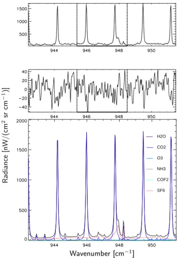
R ad ia n ce [n W /( cm 2 sr cm − 1 )] H2O CO2 O3 NH3 COF2 SF6 Wavenumber[ m 1 ℄
Fig. 1. Typical MIPAS spectrum (measured on 5 November 2003 at 12 km tangent altitude) (top), residual differences between mea-surement and best-fit spectrum (middle), and trace species spectral contributions (bottom). The bold horizontal line together with the vertical lines in the top two panels indicate the spectral range used within the retrievals. Main contributors are SF6(bold dashed red), CO2FB laser band (blue, large spectral lines) and CO2FH laser
band lines (blue, small spectral lines), and water vapour (violet).
Prior to the retrieval of SF6volume mixing ratios (vmrs),
the following quantities were retrieved and the resulting pro-files were used as a priori information in the SF6retrievals:
residual spectral shift, instrument line shape correction, tem-perature and line of sight (von Clarmann et al., 2003b), and ozone. NH3and COF2emissions were also considered in the
radiative transfer modelling, using climatological profiles for these trace species (Kiefer et al., 2002). The spectral range used for SF6 retrieval was 945.4 cm−1 to 948.5 cm−1 (see
Fig. 1). Simultaneously with SF6, CO2and H2O vmrs were
retrieved in a multi-parameter retrieval approach. Beyond this, the background continuum emission and zero radiance calibration correction were retrieved jointly. The rationale of this approach is discussed in detail in von Clarmann et al. (2003b).
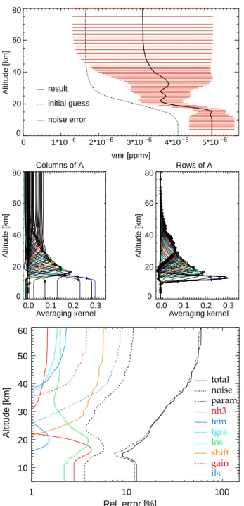
0 1*10−6 2*10−6 3*10−6 4*10−6 5*10−6 vmr [ppmv] 0 20 40 60 80 Altitude [km] result initial guess noise error Columns of A 0.0 0.1 0.2 0.3 Averaging kernel 0 20 40 60 80 Altitude [km] Rows of A 0.0 0.1 0.2 0.3 Averaging kernel 0 20 40 60 80 Altitude [km] 1 10 100 Rel. error [%] 10 20 30 40 50 60 Altitude [km] total noise param nh3 tem tgra los shift gain ils
Fig. 2. Typical profile (top), columns and rows of the averaging kernel (middle), and relative error budget (in percent) (bottom), for a measurement of 5 November 2003. All spectra below 12.7 km have been excluded from the retrieval because of cloud contam-ination (cloud index less than or equal to 6). Error sources as-sessed are measurement noise (noise),the uncertainties in temper-ature (tem), line-of-sight (los) (from preceding retrievals), NH3
(nh3)(from climatological variability), and horizontal temperature gradients (tgra), residual uncertainties in radiometric (gain) and fre-quency shift calibration (shift), and residual uncertainties in the in-strumental line shape (ils). The quadratic sum of all errors except measurement noise is given by the black dashed line (param), while the quadratic sum over all error sources is given by the black solid line (total).
In the vicinity of the SF6signatures non-local
thermody-namic equilibrium (non-LTE) effects are an important issue for the CO2lines (L´opez-Puertas and Taylor, 2001). To
cor-rect for these non-LTE emissions, but to keep the computa-tional effort reasonably low, the CO2lines of the FB and the
FH laser band, respectively, have been modelled in a first-order approach by retrieving a CO2 pseudo-vmr, i.e. a
vol-ume mixing ratio which, under LTE assumption, causes the same emission as the true CO2 vmr under non-LTE. Since
the two relevant bands are differently affected by non-LTE effects, the lines of the two bands were handled formally as if they belonged to different trace species. In order to con-strain the CO2line of the FH laser band just below the SF6
signature, further lines of the same band near 945.4 cm−1, 946.7 cm−1, and 947.1 cm−1were also fitted. An example of measured and best-fit spectra, together with the assignment of the trace species spectral signatures is shown in Fig. 1. Due to non-linearity effects in radiative transfer, adjusting the vmrs to fit a spectral line instead of adjusting the non-LTE vibrational populations of the molecular states is only an approximation. The systematic errors introduced by this approach are discussed in Sect. 3.2.
The retrieval is performed on an altitude grid of 1 km step widths up to 44 km and 2–20 km steps above, and is regular-ized by a Tikhonov-type constraint which adds to the objec-tive function of the least squares fit a penalty which keeps the differences of mixing ratios at adjacent altitudes reason-ably small (Tikhonov, 1963; Steck and von Clarmann, 2001; Steck, 2002). This is achieved by using a smoothness con-straint matrix of the type γ LT1L1where γ is a scaling factor and L1 is a first order finite differences operator. The use of the latter does not constrain the column information but only how this information is distributed over altitude and, thus, provides a bias-free retrieval. A typical profile is pre-sented in Fig. 2, upper panel, together with its uncertainties due to measurement noise. The regularization strength has been adjusted such that about 4 degrees of freedom are ob-tained within the altitude range 8–35 km, resulting in a ver-tical resolution of 4 km near the tropopause and 8 km above 35 km (see Fig. 2, middle panel). In order not to introduce any artifacts in the profile structure, an all-zero flat a priori profile has been used, which acts, along with the first order differences regularization operator, only as a smoothing con-straint. Initial guess profiles in our retrievals are distinct from the a priori profiles and stem from a climatology (Kiefer et al., 2002). Since we iterate until convergence is achieved, the initial guess profiles have no influence on the results.
Error estimation is based on linear theory as suggested by Rodgers (2000). The error budget of the profile in Fig. 2 is provided in the third panel. The error budget includes the mapping of the measurement noise on the retrieved vol-ume mixing ratios as well as the propagation of uncertainties of model parameters onto the result. Up to approximately 25 km, the total uncertainty in the SF6 vmr profiles is 0.4
dominating error source.
Additional contributions to model parameter errors were found to be uncertainties in temperature (tem), line-of-sight (los) (from preceding retrievals), NH3 (nh3) (from
climato-logical variability), horizontal temperature gradients (tgra), residual uncertainties in radiance (gain) and frequency shift calibration (shift), and residual uncertainties in the instru-mental line shape (ils). The main model parameter error con-tributions, however also of random nature, are the uncertain-ties due to the interference of NH3 lines for which the
at-mospheric volume mixing ratio is unknown, and the residual line-of-sight uncertainty. The only non-negligible systematic error source besides the spectroscopic uncertainty (reported to be a few percent (Nemtchinov and Varanasi, 2003)), is the residual instrumental line shape uncertainty which con-tributes with approximately 5% (0.2 to 0.3 pptv) to the over-all error budget above 30 km. Typicover-ally, we use data sets from at least three observational days representing one month of measurements to construct zonal mean distributions which provide, for 5◦ latitude bins, roughly 100 observations per bin, reducing the SF6standard error of the mean to 1%.
The error estimation does not include the smoothing error, nor the mapping of the smoothing error of joint fit parameters onto the SF6 profile, since both of these errors
require robust knowledge of the true covariance matrices of these species (Rodgers, 2000), which is, to our judgment, not available.
3.2 Consideration of non-LTE emissions for interfering CO2lines
As described above, the handling of differing non-LTE ef-fects for CO2 lines from different spectroscopic bands has
been treated by a simplified approach. In order to assess the systematic error potentially introduced by this approach, a limited data set (covering two days in November 2003 and January 2004) was treated with a non-LTE approach for the CO2FB and FH laser band lines using pre-calculated
popu-lations of the respective CO2 molecular states. These have
been derived within the preceding retrieval of CO for the re-spective days, since the CO retrieval requires full CO2
non-LTE modelling (Funke et al., 2007), using the GRANADA non-LTE model (Funke et al., 2001).
The non-LTE emissions of the CO2lines then were
mod-elled by making use of the non-LTE functionality of the ra-diative transfer model KOPRA (Stiller et al., 2002) imple-mented in the scientific IMK/IAA MIPAS data processor.
The simplified approach and the full non-LTE treatment (see Fig. 3) of the CO2 lines, respectively, led to different
simulations of the CO2 emission signatures in the spectral
fits, and, in turn, to systematic SF6differences. Comparison
of both approaches revealed, for both example days, a high bias in SF6 vmr for the simplified approach (0 to 0.1 pptv
or 0 to +2%) between 10 and 20 km (tropics) and 15 and
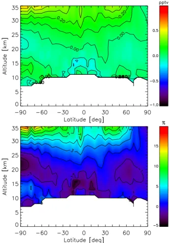
Fig. 3. Mean differences of SF6vmr profiles (top: absolute in pptv,
bottom: relative in percent) between the retrieval which fully con-siders CO2non-LTE emissions and the standard retrieval (non-LTE
– standard) for 1 January 2004. Percentage differences are given relative to the retrieval which fully considers CO2non-LTE
emis-sions, i.e. (non-LTE – standard)/non-LTE is shown. The 5◦ latitu-dinal mean differences for a full day of observations (1000 scans in total distributed within 35 latitude bands) are provided. White areas are missing data due to clouds.
25 km (high latitudes) and a low bias (0 to −0.2 pptv or 0 to −4%) at 25 to 35 km altitude. The SF6low bias is most
pro-nounced, with values of 0.5 pptv or higher, above 35 km over the summer pole due to the prevailing illumination, keeping in mind that the CO2non-LTE effects are mainly due to solar
excitation.
This means that inferred mean age of air (on the basis of a trend of 0.22 pptv yr−1) is expected to be 0 to 0.5 years
too low in the lower stratosphere and 0 to 1 year too high above 25 km; a maximum bias of up to 2 years is reached at the summer pole above 35 km only, an altitude range which is not used in this study, and not recommended to be used in other studies, for the assessment of the mean age of air. Since this effect, although of systematic nature, has no sim-ple altitude and latitude relationship, we have not corrected
the data set and use original uncorrected data for our study. Re-processing of the complete data set in order to eliminate the bias was not possible at this time due to missing CO2
vibrational temperatures (provided from CO retrievals) for most of the days included in this analysis.
3.3 Effects and handling of imperfect gain calibration
Peculiar high day-to-day variability in global SF6
distribu-tions provided another hint towards a systematic error in the data. It turned out that the SF6retrievals were extremely
sen-sitive to very small systematic oscillations in the radiance baseline, affecting the shape of the SF6signature itself and
that of interfering lines. These baseline oscillations are well below the NESR (Noise Equivalent Spectral Radiance) spec-ification of MIPAS and become visible only after averaging a huge number of spectra. Nevertheless, the SF6 retrievals,
at least above 20 to 25 km, are systematically affected by these oscillations, which occur in the version 4.61 spectra only. These radiance baseline oscillations are of different na-ture than the gain error listed in the error budget (see Fig. 2). The latter is the uncertainty of the scaling of the spectrum. A method to quantify the systematic contribution to the SF6
retrievals and to correct the SF6distributions for this
contri-bution has been developed and applied to the data set pre-sented in this study. Technical details about the correction method are given in the Appendix. For further use, daily and monthly zonally averaged SF6data have been corrected for
the systematic contributions from the radiance baseline oscil-lations according to the method described in the Appendix. All daily and monthly averages of SF6vmrs and age of air
data presented in the following sections are corrected for the bias caused by the radiance baseline oscillations (called gain-bias in the following).
4 Comparison to balloon-borne cryo-sampler data
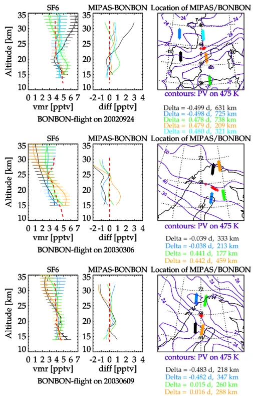
During the first observation phase of MIPAS from July 2002 to March 2004 several field campaigns took place, some of them intended for validation of Envisat instruments. The balloon-borne cryogenic whole-air sampler BONBON (En-gel et al., 2006b) which provides highly accurate data, mea-sured during three balloon flights, one on 24 September 2002 in Southern France, the other two on 6 March 2003 and 9 June 2003 near Kiruna, Sweden. Figure 4 presents the com-parison of co-incident MIPAS profiles with the in situ data, together with a map showing the locations, the temporal and spatial mis-matches and the potential vorticity (PV) fields. For close co-incidences, the MIPAS profiles agree with the BONBON data to within 0.5 pptv below 25 km which is fully consistent with the estimated error budget. For 24 Septem-ber 2002, the gain-bias corrected profiles are also shown; the gain-bias for this day is one of the smaller ones, but not neg-ligible.
5 Global SF6distributions
Global SF6distributions using gain-bias corrected data have
been derived for the period September 2002 to March 2004 for at least 3 days per month. Figure 5 shows the 5◦zonally
averaged global distribution for March 2003. For each 5◦
latitude bin, approximately 140 individual profiles have been averaged, leading to a mean value standard error in the or-der of 0.05 pptv or 1%. The zonal mean distribution reveals all features expected from earlier observations: Tropospheric SF6is homogeneously distributed with values between 5.0
and 5.5 pptv, but slightly higher in the Northern Hemisphere due to industrial sources. The SF6vmr decreases both with
altitude and latitude, reflecting the time needed to trans-port air parcels from the tropical tropopause to higher al-titudes and laal-titudes. The stratospheric SF6 vmr over the
spring pole is lowest since the aged polar vortex is filled with old air which might also have experienced SF6depletion in
the mesosphere. The seasonal and latitudinal variation of SF6within the observational data set is shown in the
elec-tronic supplement (http://www.atmos-chem-phys.net/8/677/ 2008/acp-8-677-2008-supplement.pdf) as monthly zonal mean profiles (averaged for 5◦ latitude bins) for various months and latitudes.
6 Tropical tropospheric SF6increase
The temporal tropical tropospheric increase of MIPAS SF6
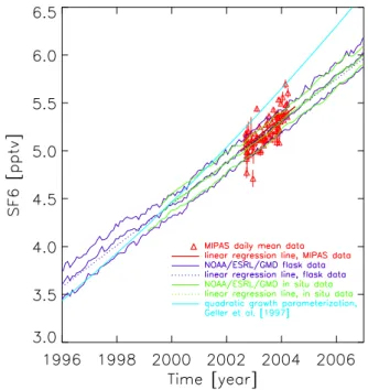
observations was derived from daily mean values averaged over 17.5◦S to 17.5◦N and 9 to 15 km (Fig. 6). The lin-ear regression provides an increase of 0.230±0.008 pptv/ylin-ear with an extrapolated value of 4.89 pptv on 1 January 2002. This is in excellent agreement with globally averaged ground-based flask and in situ observations as provided by the NOAA/ESRL/GMD (data from ftp://ftp.cmdl.noaa.gov/ hats/sf6/insituGCs/CATS/global/insitu global SF6 and ftp:// ftp.cmdl.noaa.gov/hats/sf6/flasks/SF6global 2007.txt): The trend reported for NOAA/ESRL/GMD in situ global data is 0.224±0.002 pptv/year, and for flask data it is 0.217±0.003 pptv/year; both data sets provide a global mean of 4.88±0.03 pptv for January 2002 (B. Hall, personal com-munication, 2007).
Although the NOAA/ESRL/GMD flask and in-situ data are ground-based measurements, while the MIPAS data rep-resent the tropical middle to upper troposphere, we believe that such a comparison is well justified since we expect ho-mogeneous mixing in the troposphere for a tracer like SF6
which has no tropospheric sinks. This assumption is con-firmed by findings of Gloor et al. (2007). These authors present vertical profiles of tropospheric SF6vmrs measured
in-situ at various sites and seasons (see their Fig. 7). In gen-eral, their profiles agree very well with the assumption of constant values in the planetary boundary layer (PBL) and the free troposphere. The only site where SF6vmrs in the
SF6
0 1 2 3 4 5 6 7
vmr [pptv]
10
15
20
25
30
35
Altitude [km]
BONBON-flight on 20020924 MIPAS-BONBON-2 -1 0 1 2 3 4
diff [pptv]
10
15
20
25
30
35
Location of MIPAS/BONBON -10 0 10 36 40 44 48 16 16 20 24 24 24 24 24 contours: PV on 475 K Delta = -0.499 d, 631 km SF60 1 2 3 4 5 6 7
vmr [pptv]
10
15
20
25
30
35
Altitude [km]
BONBON-flight on 20020924 MIPAS-BONBON-2 -1 0 1 2 3 4
diff [pptv]
10
15
20
25
30
35
Location of MIPAS/BONBON -10 0 10 36 40 44 48 16 16 20 24 24 24 24 24 contours: PV on 475 K Delta = -0.498 d, 725 km SF60 1 2 3 4 5 6 7
vmr [pptv]
10
15
20
25
30
35
Altitude [km]
BONBON-flight on 20020924 MIPAS-BONBON-2 -1 0 1 2 3 4
diff [pptv]
10
15
20
25
30
35
Location of MIPAS/BONBON -10 0 10 36 40 44 48 16 16 20 24 24 24 24 24 contours: PV on 475 K Delta = 0.478 d, 738 km SF60 1 2 3 4 5 6 7
vmr [pptv]
10
15
20
25
30
35
Altitude [km]
BONBON-flight on 20020924 MIPAS-BONBON-2 -1 0 1 2 3 4
diff [pptv]
10
15
20
25
30
35
Location of MIPAS/BONBON -10 0 10 36 40 44 48 16 16 20 24 24 24 24 24 contours: PV on 475 K Delta = 0.479 d, 209 km SF60 1 2 3 4 5 6 7
vmr [pptv]
10
15
20
25
30
35
Altitude [km]
BONBON-flight on 20020924 MIPAS-BONBON-2 -1 0 1 2 3 4
diff [pptv]
10
15
20
25
30
35
Location of MIPAS/BONBON -10 0 10 36 40 44 48 16 16 20 24 24 24 24 24 contours: PV on 475 K Delta = 0.480 d, 321 km SF60 1 2 3 4 5 6 7
vmr [pptv]
10
15
20
25
30
35
Altitude [km]
BONBON-flight on 20030306 MIPAS-BONBON-2 -1 0 1 2 3 4
diff [pptv]
10
15
20
25
30
35
Location of MIPAS/BONBON 64 68 72 30 40 50 contours: PV on 475 K Delta = -0.039 d, 333 km SF60 1 2 3 4 5 6 7
vmr [pptv]
10
15
20
25
30
35
Altitude [km]
BONBON-flight on 20030306 MIPAS-BONBON-2 -1 0 1 2 3 4
diff [pptv]
10
15
20
25
30
35
Location of MIPAS/BONBON 64 68 72 30 40 50 contours: PV on 475 K Delta = -0.038 d, 213 km SF60 1 2 3 4 5 6 7
vmr [pptv]
10
15
20
25
30
35
Altitude [km]
BONBON-flight on 20030306 MIPAS-BONBON-2 -1 0 1 2 3 4
diff [pptv]
10
15
20
25
30
35
Location of MIPAS/BONBON 64 68 72 30 40 50 contours: PV on 475 K Delta = 0.441 d, 177 km SF60 1 2 3 4 5 6 7
vmr [pptv]
10
15
20
25
30
35
Altitude [km]
BONBON-flight on 20030306 MIPAS-BONBON-2 -1 0 1 2 3 4
diff [pptv]
10
15
20
25
30
35
Location of MIPAS/BONBON 64 68 72 30 40 50 contours: PV on 475 K Delta = 0.442 d, 459 km SF60 1 2 3 4 5 6 7
vmr [pptv]
10
15
20
25
30
35
Altitude [km]
BONBON-flight on 20030609 MIPAS-BONBON-2 -1 0 1 2 3 4
diff [pptv]
10
15
20
25
30
35
Location of MIPAS/BONBON 64 68 72 22 22 22 24 24 24 26 contours: PV on 475 K Delta = -0.483 d, 218 km SF60 1 2 3 4 5 6 7
vmr [pptv]
10
15
20
25
30
35
Altitude [km]
BONBON-flight on 20030609 MIPAS-BONBON-2 -1 0 1 2 3 4
diff [pptv]
10
15
20
25
30
35
Location of MIPAS/BONBON 64 68 72 22 22 22 24 24 24 26 contours: PV on 475 K Delta = -0.482 d, 347 km SF60 1 2 3 4 5 6 7
vmr [pptv]
10
15
20
25
30
35
Altitude [km]
BONBON-flight on 20030609 MIPAS-BONBON-2 -1 0 1 2 3 4
diff [pptv]
10
15
20
25
30
35
Location of MIPAS/BONBON 64 68 72 22 22 22 24 24 24 26 contours: PV on 475 K Delta = 0.015 d, 260 km SF60 1 2 3 4 5 6 7
vmr [pptv]
10
15
20
25
30
35
Altitude [km]
BONBON-flight on 20030609 MIPAS-BONBON-2 -1 0 1 2 3 4
diff [pptv]
10
15
20
25
30
35
Location of MIPAS/BONBON 64 68 72 22 22 22 24 24 24 26 contours: PV on 475 K Delta = 0.016 d, 288 km ✁ ✁Fig. 4. Comparison of individual SF6profiles with co-located in situ observations obtained during balloon flights of a cryogenic whole-air sampler (BONBON) (Engel et al., 2006b), for (top) 24 September 2002 over Southern France, and (middle) 6 March 2003 and (bottom) 9 June 2003 over Northern Scandinavia. The left panels show the profiles measured by MIPAS (colours except red) and BONBON (red) for the best co-incidences. The middle panels provide the difference profiles between MIPAS and BONBON. In the right panels the location of the observations are shown together with the PV contours on 475 K (violet contour lines, PV units: K m2kg−1s−1) and the temporal and spatial distances. For the September 2002 flight, in addition the gain-bias corrected MIPAS observations are given (dashed coloured lines except red in the left panel).
Fig. 5. Global mean distribution of SF6(gain-bias corrected) for
March 2003 (geographical latitude versus altitude, 5◦latitude bins; approximately 140 profiles per latitude bin). White areas are miss-ing data due to clouds.
PBL were significantly higher than in the free troposphere was Harvard, Forest, Massachusetts (called HFM) which “is located near a strong emission region” (Gloor et al., 2007). In their Table 4, they present PBL – free troposphere dif-ferences in the order of −0.03 to +0.05 pptv, (with one ex-ception, again belonging to HFM where the difference is +0.22 pptv). Differences in the order of 0.025 pptv (about 0.5% of the actual SF6vmr) are below the standard error of
the MIPAS daily tropical tropospheric mean values and just in the range of the standard error of the GMD ground-based in-situ data and would, thus, not be detectable in the com-parison to GMD values. We conclude from the Gloor et al. (2007) paper that the bias between the PBL and the free tro-posphere is so small that it is not relevant within the MIPAS – NOAA/ESRL/GMD comparison.
The MIPAS-derived linear increase has been used to con-vert SF6global distributions into mean age of stratospheric
air by assigning the SF6vmr difference observed in the
tropo-sphere and at some location in the stratotropo-sphere, respectively, to the time lag since the troposphere had shown the mixing ratio measured in the stratosphere, according to the following linear relationship:
age = t − t0−
SF6−a
b (1)
with t =time of the observation (in years), t0=2002.0 (i.e. 1
January 2002), a=4.89 pptv (the tropical tropospheric vmr on 1 January 2002 as derived from Fig. 6), b=0.230 pptv/yr (the yearly tropical tropospheric increase as derived from Fig. 6). By doing this we implicitly assume that the yearly increase of the tropical tropospheric SF6 vmr as derived from
MI-PAS has remained linear and constant within the relevant pe-riod given by the actual ages observed in the atmosphere, i.e. for about 10 to 15 years. For about 8 years, this as-sumption is confirmed by the time series of ground-based
Fig. 6. Tropical tropospheric SF6increase derived from the daily gain-bias corrected zonal mean distributions of SF6within 17.5◦N
and 17.5◦S and 9 to 15 km altitude (red symbols and red solid line; error bars are the 1σ standard errors of the daily means). Time series of NOAA/ESRL/GMD flask measurements (violet) and in situ measurements (green) for the Northern Hemisphere (highest lines), global mean (middle lines), and Southern Hemisphere (low-est lines) are also shown, together with their regression lines for the global mean data (dotted green and violet lines). The light blue line extrapolates the growth parameterization derived by Geller et al. (1997) for the years 1987–1996 to the period 1996–2006. The trend derived from MIPAS measurements is 0.230±0.008 pptv yr−1.
NOAA/ESRL/GMD measurements covering the years 1996 to 2006, since the time series of the globally averaged SF6
vmr is well consistent with a linear increase (see Fig. 6, dot-ted lines). For the period 1987–1996, Geller et al. (1997) found that the surface SF6 increase was consistent with an
overall quadratic growth rate, where the quadratic term, how-ever, was rather small compared to the linear term (the coeffi-cients are 0.0049 pptv/yr2(quadratic term) vs. 0.2376 pptv/yr (linear term)), while Maiss and Levin (1994) found South-ern hemispheric SF6observations between 1970 and 1991 to
be consistent with a purely quadratic increase described by 0.004763×(t −1968.82)2. The extrapolation of the Geller et al. (1997) parameterization to the 1996–2006 period is shown for comparison in Fig. 6 as light-blue line. It is ob-vious that the actual yearly increase in the 1996–2006 period is smaller and more linear than the 2nd order extrapolation from the previous 10 years. For the period 1987–1996, how-ever, the extrapolation of the linear trends from MIPAS and NOAA/ESRL/GMD will overestimate the steepness of the SF6increase, introducing a systematic error into the
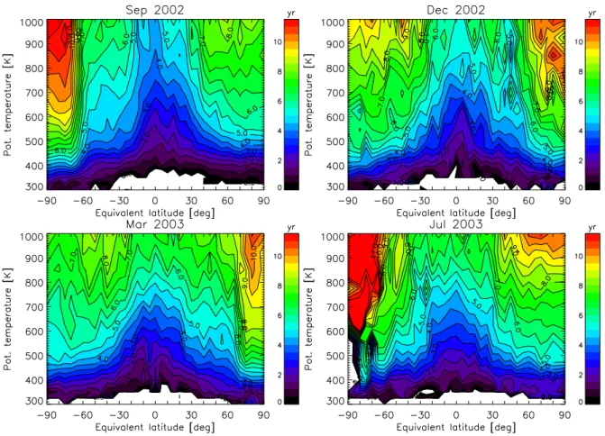
Fig. 7. Global distributions of mean age of stratospheric air (potential temperature versus equivalent latitudes) for the months September 2002 (top left), December 2002 (top right), March 2003 (bottom left), and July 2003 (bottom right).
If we assume that the SF6increase is described well by
the quadratic parameterization derived by Geller et al. (1997) for the period 1987–1996 and by the MIPAS-derived linear increase since 1996, and we use the MIPAS-derived linear increase for age-of-air assessment for ages between 6 and 15 years, we underestimate the inferred ages by at most 1.2 years, i.e. for 15 year old air the MIPAS linear increase would provide an age of 13.8 years. If we additionally cor-rect the Geller et al. growth parameterization by an addi-tive term of +0.14 pptv in order to better match the most re-cent NOAA/ESRL/GMD global mean flask data of 1 January 1996 (3.58 pptv, from the regression line), we estimate that the MIPAS linear trend will underestimate the inferred ages even by up to 1.7 years for 15 years of “real” age. However, one should keep in mind that SF6-derived ages higher than
6 to 8 years have been observed within polar vortices only; the respective low SF6 vmrs are due to intrusions of
meso-spheric air which had undergone mesomeso-spheric SF6loss
pro-cesses (see Sect. 7.3); the assessment of real age of air from these SF6observations suffers from further uncertainties like
the details of mesospheric loss modelling in chemistry trans-port models.
We used the MIPAS-derived increase instead the NOAA/ESRL/GMD trend in order to account for the small additive bias between MIPAS and the ground-based mea-surements which is apparent by the vertical shift of the MI-PAS regression line (red solid line in Fig. 6) versus the NOAA/ESRL/GMD global mean time series (middle green and violet solid lines and dotted regression lines in Fig. 6).
7 Mean age of stratospheric air
7.1 Global distributions
The global distribution of the mean age of stratospheric air derived from MIPAS SF6monthly zonal means (provided for
potential temperature versus equivalent latitudes) is shown in Fig. 7 for the months September 2002, December 2002, March 2003, and July 2003. While ascent of young air is most pronounced over the tropics during the Northern Hemi-spheric fall and winter months (Fig. 7, top row), very old air is found for both polar winter vortices (top and bottom right panels). During fall (top and bottom left panels) in the respective hemisphere, the horizontal age gradients in the
Fig. 8. Mean age of air at (top) 16 km, (middle) 20 km, and (bot-tom) 25 km altitude from MIPAS/Envisat SF6 distributions;
pre-sented are the monthly zonal means for 5◦ latitude bins for all months between September 2002 and March 2004. The error bars represent the 1σ standard errors of the mean.
middle stratosphere are lowest, providing ages typical for mid-latitudes also in the polar regions. During spring (top and bottom left panels) the surf zone in mid-latitudes is most pronounced revealing latitudinally nearly constant mean age
of air in the lower to middle stratosphere, which is produced by isentropic mixing due to planetary waves.
The surf zone is separated from the tropics, and even more sharply separated from the polar vortex, by a barrier reveal-ing very high horizontal age gradients. Also remarkable is the remnant of old air in the middle stratospheric summer above 850 K during December 2002 (NH) and July (SH) (Fig. 7, top and bottom right panels).
A compilation of monthly zonally averaged age of air dis-tributions at three different altitudes is shown in Fig. 8. In the tropics and mid-latitudes, the seasonal variation over the 19 months covered by our data is rather low. Similar fig-ures are available from, e.g. NASA ER-2 observations of the mean age of air (see, for example, Waugh and Hall (2002), their Fig. 6); the MIPAS results can be compared directly with those and provide, additionally, data for the Southern Hemisphere polar region. For 20 km altitude, the tropical mean age of air from MIPAS is between 0.5 and 2.5 years while the ER-2 observations yield an age around 1 year. The mean age increases with latitude for both hemispheres, with a significant seasonal variation in the polar regions. During polar winter on the Northern Hemisphere, the highest MI-PAS values are around 6 years, while near the South pole, the spread is considerably larger with SF6-derived apparent
ages of up to 9.5 years in winter and spring. From the ER-2 data set, Northern Hemispheric ages of up to 6 years, and 60◦S ages up to 5.5 years were derived, which are consistent with our data set. Inter-annual differences are also notice-able (compare, for instance, September 2002 to September 2003). During September 2002 an unprecedented Southern hemispheric major warming took place, with very high plan-etary wave activity (Manney et al., 2005b) which might be reflected in the slightly unusual age of air distribution. For 16 km altitude (first panel of Fig. 8), i.e. just at the altitude of the tropical tropopause layer, the age of air in the tropics is between 0 and 1.5 years, as expected. For polar regions, ages between 2 and 5 years in the North and 3 to 7 years in the South are observed. For higher altitudes (e.g. 25 km, third panel of Fig. 8) the tropical mean age of air is around 3 to 3.5 years, while the seasonal variation and inter-annual differences at the poles become even more pronounced; this suggests stronger impact of mesospheric intrusions at this al-titude than lower down in the stratosphere (see below). The systematic bias in the present MIPAS age data set due to the CO2non-LTE treatment (see Sect.3.2 and Fig. 3) should be
kept in mind for these comparisons. A complete correction of this bias is not possible at the current state since its seasonal variation is not yet known. For Northern winter conditions (see Fig. 3), correction of the bias would increase the age of air at 16 km by about 0.5 years in the tropics and 0 to 0.5 years at other latitudes; it would not change the latitudinal distribution at 20 km; and it would decrease the age of air by about 0.5 years for all latitudes at 25 km.
Zonally averaged monthly mean profiles of mean age of air for several latitudes and months, similar to Waugh
and Hall (2002), their Fig. 6, are provided in the elec-tronic supplement (http://www.atmos-chem-phys.net/8/677/ 2008/acp-8-677-2008-supplement.pdf).
7.2 Temporal variation
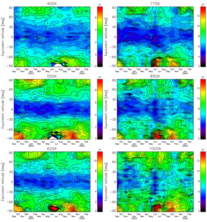
The seasonal variation and inter-annual differences are most clearly displayed by time series of equivalent-latitude distri-butions at certain potential temperature levels (see Fig. 9) and those of vertical profiles (in terms of potential temperature as vertical coordinate) for certain equivalent-latitude bands (see Fig. 10). During Austral winter, extremely high appar-ent ages of 12 years or more, in fact unrealistically high, were observed at the 625 K surface and above (see Fig. 9 and Fig. 10, bottom panel) during two episodes (June to July 2003; September to November 2003), separated by an episode of younger air (August 2003). The first episode of high mean age started rather abruptly in June 2003; in July the polar vortex was filled with air older than 8 years, south of 70◦S equivalent latitude for altitudes above the 675 K po-tential temperature level. After the break in August 2003, the latitude- and altitude regime filled up with old air even increased; this situation lasted until end of November. The Antarctic winter 2003 has been characterized from observa-tions of CO (Funke et al., 2005) and NOx(Funke et al., 2005;
Randall et al., 2007) by a very strong vortex with long-lasting and strong transport of mesospheric air into the stratospheric vortex. Hence, the very high apparent age of air observed is most probably due to SF6-depleted mesospheric air masses
filling the stratospheric vortex. In contrast to the very long-lasting area of old air masses in 2003, the very old air disap-peared earlier in 2002, probably due to the weak vortex being perturbed frequently by planetary wave activity which finally led to the first observed Southern Hemispheric major warm-ing (Manney et al., 2005b). Although very high ages were no longer observed during Southern summer, the mean age of air remained rather high even then, with values around 6 to 8 years. Only immediately before the formation of the next polar vortex, in April/May, ages closer to those typical for mid-latitudes were observed at high Southern latitudes, indi-cating that polar summer air was mixed with lower-latitude air.
The observed northern hemispheric winters 2002/2003 and 2003/2004 are rather different than the Southern hemi-spheric ones (2002 and 2003) since obvious subsidence episodes are shorter, and the high ages of the Southern hemi-spheric winters have not been observed (Fig. 9 and Fig. 10, top panel). At 625 K, the highest age of air observed in the Northern winters during the measurement time of MI-PAS is 8 to 9 years, in March 2003 and 2004; ages of 10 or more years are observed at 1000 K in December 2002, March 2003, January and March 2004, and, surprisingly, in July 2003. Intrusions of mesospheric air into the polar vortex during the Northern winter 2002/2003 are described in vari-ous papers (Konopka et al., 2007; Engel et al., 2006b). This
seems to be confirmed by MIPAS age of air observations. However, although the 8-year isoline came down to about 550 K in December 2002, the mesospheric intrusion did ob-viously not last long enough to fill up the vortex with aged mesospheric air. Another extreme winter was the late winter 2004 (Manney et al., 2005a; Randall et al., 2006). During January to March 2004, strong subsidence of upper atmo-spheric NOx into the polar stratosphere has been observed
by various instruments (Randall et al., 2006; Sepp¨al¨a et al., 2007; Hauchecorne et al., 2007; Funke et al., 20081). This again is confirmed by the observed age of air, since ages of 8 years and more have been observed above 625 K. However, despite severe subsidence events, similar high ages of air as for the Southern hemispheric winter 2003 have not been ob-served during the two Northern hemispheric winters covered by MIPAS (see Fig. 9). Considerable inter-hemispheric dif-ferences are also observed at high latitudes at the 400 K level (see Fig. 9, top left panel), with air again being much older in the Southern Hemisphere.
The age of air in the tropics at 400 K is rather constant over the seasons, except that a slight seasonal oscillation with lat-itudes can be observed. At 850 and 1000 K, however, the tropical air is youngest in Northern winter 2002/2003, but even Northern winter 2003/2004 (December 2003 to Febru-ary 2004) has younger air than the summer and fall months before, except June 2003. Observation of younger air at tropical high altitudes during northern winter months is con-sistent to the fact that the strongest ascent by the Brewer-Dobson circulation occurs during this time of the year. In June 2003, very young air (i.e. strong upwelling) is found in the tropics which might be related to the very old air at the South pole (strong subsidence), indicating a short episode of intensified circulation.
7.3 Comparison to model calculations
Observations of apparent age of air derived from SF6vmrs
of more than 6 to 8 years were also reported previously (En-gel et al., 2006b; Hall and Waugh, 1998; Waugh and Hall, 2002). However, other age of air tracers like CO2do not
con-firm these high ages; the mesospheric loss of SF6 is
gener-ally considered to explain this discrepancy (Hall and Waugh, 1998; Reddmann et al., 2001). In order to confirm that the high mean age values derived from MIPAS observations dur-ing polar winters can be explained by the mesospheric sink of SF6, we performed model simulations with the Karlsruhe
Simulation model of the Middle Atmosphere (KASIMA), a 3D-chemistry transport model which includes a module for SF6chemistry in the mesosphere (Reddmann et al., 2001).
SF6is mainly destroyed via electron attachment and
subse-quent transformation to HF.
1Funke, B., L´opez-Puertas, M., Stiller, G., von Clarmann, T.,
Grabowski, U., and Linden, A.: Upper atmospheric NOxintrusions
into the Arctic stratosphere during January to April 2004, to be sub-mitted, Atmos. Chem. Phys. Discuss., 2008.
Fig. 9. Global time series of zonal distributions of the mean age of stratospheric air (versus equivalent latitude) at 400 K (left column, top), 550 K (left column, middle), 625 K (left column, bottom), 775 K (right column, top), 850 K (right column, middle), and 1000 K (right column, bottom), constructed from monthly means. Note the different colour scales in the panels. The white areas in the 400 K and 550 K panels are due to missing data due to clouds (PSCs).
For the present studies, the model version as described in Reddmann et al. (2001) is applied, but using ERA-40 analy-ses up to 18 km, a relaxation term up to 1 hPa and the prog-nostic part of the model above. From the lower pressure height boundary at 7 km up to 22 km, the vertical resolution
is 750 m. From 22 km up to the upper boundary at 120 km, the vertical spacing between the levels gradually increases to 3.8 km. The triangular truncation, T21, used corresponds to a horizontal resolution of about 5.7◦×5.7◦. A numerical time step of 12 min was used in the experiments.
Fig. 10. Time series of mean age of stratospheric air vertical pro-files (constructed from monthly zonal means) (potential tempera-ture as vertical coordinates) for the equivalent latitude bands 60◦N– 90◦N (top), 20◦S–20◦N (middle), and 90◦S–60◦S (bottom).
As described in Reddmann et al. (2001) assumptions on the free thermal electron density and the reaction constants used influence the results. Here we use a ionisation model and include all back reactions, corresponding to an atmo-spheric lifetime of about 4500 years.
Fig. 11. Zonal mean distribution of mean age of stratospheric air for October 2003 from MIPAS (top), and KASIMA with (middle) and without (bottom) consideration of the SF6loss reaction in the
mesosphere, giving the apparent and the true mean age, respec-tively.
Figure 11 compares the monthly global mean distribu-tion of MIPAS age of air for October 2003 (top panel) with KASIMA calculations including (middle panel) or
disregard-ing (bottom panel) the mesospheric sink reaction. For the simulation with mesospheric loss, the apparent ages pro-duced over the South pole are much closer to the MIPAS ob-servations. In fact, the age of air calculated from this model run is 12 years or more, in very good agreement with the MIPAS observations. In contrast, treating SF6as a fully
sta-ble tracer produces ages around 6 to 8 years over the South pole which has to be considered as the real transport time. This comparison confirms the assumption that high apparent ages as derived from SF6are due to transport of SF6-depleted
mesospheric air into the stratosphere.
The MIPAS time series show that such mesospheric intru-sions are quite a frequent phenomenon. Further, the com-parison roughly confirms the atmospheric lifetime of SF6
as-sessed by this study to be about 4500 years. Finally, the im-portance of the mesospheric SF6 sink is emphasized when
comparing chemistry-transport models with age of air data derived from SF6. A more detailed analysis of the MIPAS
data set together with model simulations of the global mean age of air distribution is planned for the near future.
8 Conclusions
We have derived mean age of air global distributions for the altitude range 6 to 35 km and the period September 2002 to March 2004 from MIPAS/Envisat SF6 observations with a
precision (in terms of the standard error of monthly 5◦zonal means based on approximately 100 single observations each) of 0.25 yr. The systematic error of the mean age of air data set is ruled by the uncertainty in spectroscopic data and a simplified non-LTE treatment in the SF6retrieval approach
which both might explain a potential bias of up to 1 year for altitudes below 35 km (up to 2 years above 35 km), at certain latitudes and seasons. Comparison to previous observations reveals that the SF6and mean age of air distributions from
MIPAS are in very good agreement with those which indi-cates that the actual systematic error is considerably lower than its estimate. The available age of air data set gives the unprecedented opportunity to validate the transport schemes in chemistry-transport and chemistry-climate models.
The global data set from MIPAS for the period September 2002 to March 2004 reveals high seasonal variations and pro-nounced inter-hemispheric and inter-annual differences. In particular, in both polar vortices, frequent and, for the South-ern Hemisphere, long-lasting intrusions of mesospheric air into the stratospheric vortex are observed, identified by very high apparent mean ages of 8 to 12 years and higher. The fre-quent mesospheric intrusions seen in MIPAS data may have been underestimated in the past and their role on chemistry-climate coupling needs further assessment. The mesospheric depletion of SF6has been confirmed as source of the
overes-timation of the mean age of air by comparison of the obser-vations with model calculations including and disregarding, respectively, the mesospheric chemical sink reactions of SF6.
Since MIPAS data contain independent information to quan-tify subsidence of mesospheric air (via CO or CH4, cf. Funke
et al., 2005), the mesospheric sink strength, which is coupled to the mesospheric electron density, can be unambiguously quantified. This will help to improve the age of air assess-ment from SF6and to make it more consistent with age of air
estimates based on other tracers.
SF6 distributions discussed in this paper were retrieved
from MIPAS high resolution spectra recorded in the origi-nal measurement mode between September 2002 and March 2004 before an instrument failure forced spectral degrada-tion. The high seasonal variation and inter-annual differ-ences observed are an obstacle to the unambiguous detection of a change in middle atmospheric global circulation from the currently available data set. However, 5 years of MIPAS level 1-B data are now available, and an extension of the mis-sion for another 3 to 7 years is planned. This will provide a tremendous amount of information, assuming an equally ac-curate SF6retrieval will be possible from the reduced
spec-tral resolution data, which still has to be proven.
Appendix A
Correction of SF6 vmr biases caused by inadequate gain calibration
The original MIPAS time series of SF6is characterized by
occasional unphysical values, which form secondary modes in the histogram of SF6 daily mean values. In order to
re-ject or correct unrealistic values from the assessment of the age of the air without running risk of rejecting/correcting any true but unexpected data caused by unknown chemistry or physics, a search was made for an external data filter which is independent of the SF6values themselves. Since
discon-tinuities in SF6mixing ratios were found to coincide exactly
with the changes of the MIPAS gain calibration function, it was necessary to further assess the MIPAS calibration char-acteristics in the SF6 microwindow. MIPAS radiance
cali-bration is done by application of one gain calicali-bration func-tion over a period of typically several days. For all limb se-quences within such a gain calibration period, the spectra of the uppermost tangent altitude (approximately 68 km) were averaged over time. This was done separately for spectra recorded during forward and backward movement of the in-terferometer mirrors, because calibration is done separately for forward and backward measurements.
Since, except for the two CO2FB laser band lines, all other
atmospheric signals (e.g. CO2laser hot band lines, CO2
iso-tope transitions, H2O, SF6) are too weak to be noticeable,
zero signal is expected in the gaps between the two promi-nent CO2lines in the averaged spectra. Instead, for several
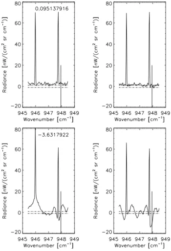
gain calibration periods, systematic deviations from the zero radiance level were observed in version 4.61 spectral data (see Fig. 12). The amplitude of this error in the calibrated
Fig. 12. Averaged radiance spectra of the highest tangent altitudes (i.e. approximately 68 km) in the region of the SF6signature for an
example of close-to-perfect (top) and heavily distorted radiance cal-ibration (bottom), respectively. The spectra were averaged over the period when one specific gain calibration function was applied; this is 8 to 9 December 2002 for the top panel and 28 to 30 April 2003 for the bottom panel. Averaging was done for forward (left) and backward (right) sweeps separately. The horizontal dashed lines in-dicate the expected NESR for the averaged spectra. The vertical solid line gives the position of the SF6peak. The number provides
the value of the gain index derived (for further details see text).
spectra is below the NESR of a single spectrum, and within the MIPAS radiance calibration specifications, but clearly visible in the averaged spectra.
Since the gain calibration functions are applied multiplica-tively, it is not quite obvious how zero radiances can be af-fected and one might tend to attribute this artifact to the (ad-ditive) offset calibration function. The latter, however, is updated several times per orbit and does not coincide with the changes of the observed artifact. Thus, the nature of the detected artifact is still unexplained; since the details of the implementation of the calibration algorithm are beyond our direct control, we restrict ourselves to correcting the affected SF6vmr data.
Fig. 13. Correlation between orbit-averaged SF6vmrs and
orbit-related gain indices for the altitude level 25 km. The vertical lines are the standard errors of the orbit means. The text provides the abscissa [pptv], slope, correlation coefficient, and altitude [km].
In a transparent atmosphere where radiative transfer is linear, and when measurement noise is equally distributed within the spectral gridpoints under consideration, the map-ping of a systematic measurement error on the retrieved tar-get mixing ratio is proportional to the product of the row vector containing the typical target spectral signal and the column vector containing the spectral error. Thus we esti-mate the retrieval error due to baseline oscillations caused by inadequate radiance calibration, in arbitrary units, as
1SF6=c × N X n=1 ySF6;n× (A1) (yart.,fw;n+yart.,bw;n− PN n=1yart.,fw;n N − PN n=1yart.,bw;n N )
where n runs over all N spectral gridpoints of the SF6
mi-crowindow except those where the prominent CO2laser band
lines are situated. c is a constant of the dimension [pptv (W/(cm−2sr cm−1))−2]; ySF6;n is the spectral signal of the
SF6band, and yart.,fw;nand yart.,bw;nare the systematic
radi-ance errors at spectral gridpoint n in the forward and back-ward spectra, respectively. The subtraction of the average background signal accounts for the average offset correction in our retrieval (von Clarmann et al., 2003b). This 1SF6
value, further referred to as gain index, was used as measure of the impact of erroneous gain calibration in further correc-tion steps. In total, 87 gain calibracorrec-tion periods were analyzed by means of the spectral analysis described above, all of them applied within the period September 2002 to end of March 2004, and 87 gain indices were derived.
For correction of the SF6vmrs derived from v4.61
spec-tral data and distorted by imperfect radiance calibration, SF6
global means (90◦S–90◦N) per orbit for all altitude levels for two height grids, from 44 km to 7 km and 1500 K to
Fig. 14. Time series of SF6 zonal mean distributions at 25 km
altitude before (top) and after (bottom) correction for the bias due to inadequate radiance calibration. Remnants of the gain-calibration caused artifacts remained for some days and regions, particularly for high Southern latitudes on 29 April 2003, 7 May 2003, and 27 July 2003, and for high Northern latitudes for some days during November 2003. White areas indicate SF6values below 2.5 pptv or
missing data due to clouds (PSCs).
350 K, were calculated. These orbit mean values for each altitude were correlated with the gain indices derived for the respective orbits. A linear relationship between orbit-mean SF6 vmrs and gain indices was established for all altitudes
and potential temperature levels (see Fig. 13). From the lin-ear regression of this correlation an additive correction term for each altitude or potential temperature level was derived. For all daily and monthly mean distributions, each SF6value
derived from v4.61 spectral data has been corrected by the following expression
SF6korr(z, orbit) = SF6original(z, orbit)− (A2)
a(z) × gain index(orbit)
with a(z) being the altitude dependent slope of the lin-ear regression (SF6 vs. gain index) (see Fig. 13) and
gain index(orbit) the orbit-dependent gain index character-izing the error due to inadequate gain calibration. a(z) is of
the order of 1.0 for 44 km altitude and decreases smoothly to values around 0.06 for 10 km, while the gain index varies between −4.0 and +2.5 for the gain calibration periods under investigation. For SF6means built from more than one gain
calibration periods, the weighted mean of the gain indices was applied.
It should be noted that the method described above could lead to an unwanted artificial component in the temporal vari-ation of SF6 in terms of seasonal variation or trend, if the
gain index varied systematically with time as well. The lat-ter, however, has been falsified, i.e. it was found that the gain index varied randomly with time rather than systematically.
Within this work, scientific analysis of SF6distributions,
and, in particular, the derivation of the tropospheric trend and mean age of stratospheric air, is based on the corrected SF6
data derived from v4.61 spectral data; the SF6vmr derived
from v4.62 spectral data are used without correction. Fig-ure 14 presents the time series of global SF6at 25 km altitude
before and after correction. In summary, while the correction is substantial, the expected SF6vmr values or any expected
structures are never used in the correction scheme. Instead, the correction relies fully and solely on the detected gain cal-ibration peculiarities.
Acknowledgements. Re-processed MIPAS level 1-B data were
provided by ESA for scientific analysis. The research work of the IMK MIPAS/Envisat group has been funded by EC via the Integrated Project SCOUT-O3 (contract No. 505390-GOCE-CT-2004), BMBF via project No. 50EE0512, and the German Research Foundation (DFG) within the Program of Emphasis CAWSES via project STI 210/4-1. We gratefully acknowledge the provision of SF6 surface flask and in situ measurements by the National
Oceanic and Atmospheric Administration Earth System Research Laboratory, Global Monitoring Division, and helpful comments on the manuscript by B. Hall.
Edited by: M. Dameris
References
Andrews, A. E., Boering, K. A., Daube, B. C., Wofsy, S. C., Loewenstein, M., Jost, H., Podolske, J. R., Webster, C. R., Her-man, R. L., Scott, D. C., Flesch, G. J., Moyer, E. J., Elkins, J. W., Dutton, G. S., Hurst, D. F., Moore, F. L., Ray, E. A., Romashkin, P. A., and Strahan, S. E.: Mean ages of stratospheric air derived from in situ observations of CO2, CH4, and N2O, J. Geophys. Res., 106, 32 295–32 314, doi:10.1029/2001JD000465, 2001. Austin, J. and Li, F.: On the relationship between the strength of
the Brewer-Dobson circulation and the age of stratospheric air, Geophys. Res. Lett., 33, L17807, doi:10.1029/2006GL026867, 2006.
Boering, K. A., Wofsy, S. C., Daube, B. C., Schneider, H. R., Loewenstein, M., Podolske, J. R., and Conway, T. J.: Strato-spheric Mean Ages and Transport Rates from Observations of Carbon Dioxide and Nitrous Oxide, Science, 274, 1340–1343, doi:10.1126/science.274.5291.1340, 1996.