Simultaneous beat and downbeat-tracking using a probabilistic framework : theory and large-scale evaluation

HAL Id: hal-00655779

https://hal.archives-ouvertes.fr/hal-00655779v2

Submitted on 22 Mar 2016

HAL is a multi-disciplinary open access

archive for the deposit and dissemination of

sci-entific research documents, whether they are

pub-lished or not. The documents may come from

teaching and research institutions in France or

abroad, or from public or private research centers.

L’archive ouverte pluridisciplinaire HAL, est

destinée au dépôt et à la diffusion de documents

scientifiques de niveau recherche, publiés ou non,

émanant des établissements d’enseignement et de

recherche français ou étrangers, des laboratoires

publics ou privés.

probabilistic framework : theory and large-scale

evaluation

Geoffroy Peeters, H Papadopoulos

To cite this version:

Geoffroy Peeters, H Papadopoulos. Simultaneous beat and downbeat-tracking using a

probabilis-tic framework : theory and large-scale evaluation. IEEE Transactions on Audio, Speech and

Lan-guage Processing, Institute of Electrical and Electronics Engineers, 2011, 19 (6), pp.1754-1769.

�10.1109/TASL.2010.2098869�. �hal-00655779v2�

Simultaneous beat and downbeat-tracking using a

probabilistic framework: theory and large-scale

evaluation

Geoffroy Peeters and Helene Papadopoulos

Abstract—This paper deals with the simultaneous estimation of beat and downbeat location in an audio-file. We propose a probabilistic framework in which the time of the beats and their associated beat-positions-inside-a-measure role, hence the downbeats, are considered as hidden states and are estimated simultaneously using signal observations. For this, we propose a “reverse” Viterbi algorithm which decodes hidden states over beat-numbers. A beat-template is used to derive the beat observation probabilities. For this task, we propose the use of a machine-learning method, the Linear Discriminant Analysis, to estimate the most discriminative beat-templates. We propose two observations to derive the beat-position-inside-a-measure observation probability: the variation over time of chroma vectors and the spectral balance. We then perform a large-scale evaluation of beat and downbeat-tracking using six test-sets. In this, we study the influence of the various parameters of our method, compare this method to our previous beat and downbeat-tracking algorithms, and compare our results to state-of-the-art results on two test-sets for which results have been published. We finally discuss the results obtained by our system in the MIREX-09 contest for which our system ranked first for the “McKinney Collection” test-set.

Index Terms—Beat-tracking, Downbeat, Beat-templates, Lin-ear Discriminant Analysis, hidden Markov model, reverse Viterbi decoding.

I. INTRODUCTION

B

challenging subjects in the music-audio research commu-nity. This is due to their large use in many applications: beat/ downbeat-synchronous analysis (such as for score alignment or for cover- version identification), beat/ downbeat-synchronous processing (time- stretching, beat- shuffling, beat- slicing), music analysis (beat taken as a prior for pitch estimation, for onset detection or chord estimation) or visualization (time-grid in audio sequencers). This is also due to the complexity of the task. While tempo estimation is mainly a problem of peri-odicity detection (with the inherent octave ambiguities), beat-tracking is both a problem of periodicity detection and a prob-lem of location of the beginning of the periods inside the signal (with the inherent ambiguities of the rhythm itself). Downbeat location is mainly a perceptual notion arising from the music construction process. Considering that the best results obtained in the last Audio Beat Tracking contest (MIREX-09) are far from being perfect, this problem is far from being solved. If most beat-tracking algorithms achieve good results for most

G. Peeters and H. Papadopoulos are with the Sound Analysis/Synthesis Team of Ircam - CNRS STMS, 1 pl. Igor Stravinsky 75004 Paris, France (see http://www.ircam.fr).

rock, pop or dance music tracks (except for highly compressed tracks), this is not the case when considering classical, jazz, world music or recent Western mainstream music styles such as Drum’n’Bass or R’n’B (which use complex rhythms).

In the following, we review related works in beat and downbeat-tracking, we review our previous beat and downbeat-tracking algorithms, we then present our new al-gorithm and compare it to existing works, we details each part of our new algorithm and finally perform a large-scale evaluation.

A. Related works

Related works in beat-tracking: This paper deals with beat-tracking from audio signal. We consider tempo period and meter has input parameters of our system and deal with audio data. Numerous good overviews exist in the field of tempo estimation or beat-tracking from symbolic data (see for example [1] [2]). We mainly reviews here existing approaches related to beat-tracking from audio signal.

Methods can be roughly classified according to the

frontend of the model. Two types of frontfrontends can be used: -discrete onset representation extracted from the audio signal (Goto [3] [4], Dixon [5]), or - continuous-valued onset func-tion (Scheirer [6], Klapuri [7], Davies [8]).

They can also be classified according to the model used

for the tracking. Goto [9] and Dixon [5] use a multi-agents model. Each agent propagates an assumption of beat-period and beat-phase, a “manager” then decides about the best agents. Scheirer [6] and Jehan [10] use resonating comb-filers which states provides the phase hence the beat information. Klapuri [7] extends this method by using the states as input to a hidden Markov model tracking phase evaluation. Probabilistic formulations of the beat-tracking problem are also proposed. For example Cemgil [11] proposes a Bayesian framework for symbolic data, it is adapted and extended to the audio case by Hainsworth [12]. Laroche [13] proposes the use of dynamic programming to estimate simultaneously period and beat-phase. Dynamic programming is also used by Ellis [14] to estimate beat-phase given tempo as input. Mixed approaches are also proposed. For example Davies [8] mixes a comb-filterbank approach with a multi-agent approach (he uses two agents representing a General State and Context-Dependent State). Most algorithms relying on histogram methods for beat-period estimation use a different algorithm for beat-phase estimation (Seppanen [15], Gouyon [16]). This is because his-togram does not provides phase information. However, recent

approaches succeed to use directly the phase information to derive beat-phase (Autocorrelation Phase Matrix of Eck [17], mid-level representation of Grosche [18]).

Finally, we can classify them according to the method

used to associate a beat likelihood to a time. Existing algorithms either use directly the values of the discrete onsets (or of the continuous onset function) at the specific time, or compute a cross-correlation between the local discrete onset sequence (or local continuous onset function) and a beat-template representing the theoretical pulses corresponding to the local tempo.

For a long time, the performances of the various

ap-proaches have been difficult to compare because authors were using different test-sets and different evaluation rules. Only recently, common test-sets (such as the ones used in [7] and [12]) and evaluation rules (such as the ones collected by [19]) have allowed this comparison. Also, the IMIRSEL team, has provided MIREX evaluation frameworks for audio beat-tracking in 2005 [20], 2006 [21] and 2009 [22] through MIREX contests. Among the top-ranked participants to these contests are (in alphabetical order): Alonso, Davies, Dixon, Ellis, Eck, Gouyon, Klapuri, Uhle.

Related works in downbeat-tracking: Most of the

proposed approaches for downbeat detection rely on prior knowledge (such as tempo, time-signature of the piece or hand-annotated beat positions). The system of Allan [23] relies upon the assumption that a piece of music will contain repeated patterns. It presents a model that uses autocorrelation to determine the downbeats given beat-positions. It has been tested on 42 different pieces of music at various metrical levels, in several genres. It achieves a success rate of 81% for pieces in 4/4 time-signature and needs more testing on 3-based time-signatures. The model of Jehan [24] is tempo independent, does not require beat tracking but requires prior knowledge acquired through listening or learning during a supervised training stage where downbeats are hand-labeled. The model has only been applied to music in 4/4 meter. Goto [25] proposes two approaches to downbeat estimation. For percussive music, the downbeats are estimated using rhythmic pattern information. For non-percussive music, the downbeats are estimated using chord change information. Klapuri [7] proposes a full analysis of musical meter into three different metrical levels: tatum, tactus and measure level. The down-beats are identified by matching rhythmic pattern templates to a mid-level representation. Ellis [26] uses a similar “template-based” approach in a drum-pattern classification task. Davies [27] proposes an approach based on a spectral difference between band-limited beat-synchronous analysis frames. The sequence of beat positions of the input signal is required and the time-signature is to be known a priori. A recent method that segments the audio according to the position of the bar lines has been presented in Gainza [28]. The position of each bar line is predicted by using prior information about the position of previous bar lines as well as the estimated bar length. The model does not depend on the presence of percussive instruments and allows moderate tempo deviations.

B. Presentation of our previous system

1) Tempo/ meter estimation system: This paper concerns the beat and downbeat-tracking problem. For this, we con-sider as input parameters an onset-energy-function f(t), time-variable tempo bpm(t) = 60/Tb(t) and meter (2/4, 3/4 or 6/8). The onset-energy-function has a sampling rate of 172Hz (step of 5.8ms). It is computed using a reassigned-spectral-energy-flux function (RSEF). The system used for the estimation of these input parameters is the one described in [29]. This system has been positively estimated in [29] and in

the MIREX-05 contest [20] for tempo estimation1_.

2) Previous tracking algorithm: Our previous beat-tracking algorithm was inspired from a P-sola analysis method for locating the Glottal Closure Instants (GCIs) [30]. This method proceeds in two separated stages. The first stage locates a set of local maxima of f(t) with an inter-distance close to the local estimated tempo period Tb(t). The second stage performs a least-square optimization in order to satisfy simultaneously two constraints: c-a) “markers close to the local maxima”, c-b) “inter-distance between markers close to Tb(t)”. We refer the reader to [31] for more details about this method, which we call P-sola in the following.

3) Previous downbeat-tracking algorithm: Our previous downbeat-tracking algorithm was based on a chord-detection algorithm [32]. This algorithm takes as input the location of the beat-markers, and computes for each beat, a chroma vector using Constant-Q transform. The chord succession is then obtained using an hidden Markov model given the observed chroma, chord emission and chord transition probabilities. The downbeats are estimated using the assumption that chords are more likely to change on the downbeat positions.

C. Paper contribution and organisation

In this paper, we present a probabilistic framework for the simultaneous estimation of beat and downbeat location given estimated tempo and meter as input.

In part II, we propose a probabilistic framework for this using a hidden Markov model formulation in which beat-times and their associated beat-position-in-measure (bpim) are the hidden states. We give the big picture in II-A, present the HMM formulation in part II-B and the specific reverse Viterbi decoding algorithm in part II-C.

We then details the various part of the model: initial probability (part III), emission probabilities (par IV), transition probabilities (part V). The emission probabilities are estimated using a beat observation probability and bpim observation probabilities. In part IV-A, we propose, for the beat obser-vation probability, the use of a machine learning approach to estimate the best beat-templates. In part IV-B, we propose, for the bpim observation probability, the use of two observations: based on the analysis of chroma vectors variation over time (part IV-B1) based on the analysis of spectral balance (part IV-B2). In part V, we present the transition probabilities which take into account the fact that hidden states represent beats in specific beat-position-in-measure.

1_{In MIREX-05, our tempo evaluation system ranked first with 95.71% in}

Finally in part VI, we propose a large-scale evaluation of beat and downbeat tracking using six different test-sets. We compare our results to state-of-the-art results and discuss the results obtained by our algorithm during the MIREX-09 contests.

Comparison to related works: Our algorithm works with a continuous onset-function rather than a series of discrete onsets. The method used to associate a beat likelihood to a time is a beat-template method. We propose a method to train the most discriminative beat-templates by using Linear Dis-criminant Analysis (LDA). This is an important contribution of this paper. As we will see, the LDA-trained beat-templates allows improving estimation results over the results obtained with more simple beat-templates representing the theoretical pulses corresponding to the local tempo [33].

The simultaneous estimation of beat and downbeat is then formulated as a hidden Markov model in which hidden states are the beat-times and their associated beat-position-in-measure. The concept of beat-position-in-measure and the use of it to derive the downbeat is inspired by the authors previous works [32], [34]. The use of a probabilistic formulation has some links with the Bayesian framework of Cemgil [11] and Hainsworth [12] but the formulation is here very different and used to perform simultaneous beat and downbeat-tracking. The formulation of hidden-states as beat-times can be linked with Laroche [33] and Ellis [14] dynamic programming approaches, especially concerning the decoding algorithm. However, in the present work, we provide a probabilistic formulation using a hidden Markov model which allows the extension of the hidden states to the down-beat estimation problem. It should be noted that our use of hidden Markov model is not related to the way Klapuri [7] uses it. In [7], two independent hidden Markov models, which hidden states represent phase evaluation, are used to track separately beat and downbeat phase.

In our system two observation probabilities are used to compute the beat-position-in-measure. They are coming from the analysis of chroma vectors variation over time and spec-tral balance (representing typical pop/ rock rhythm patterns through the time evolution of the spectral distribution). These can be linked to the works of Goto [3], [4] or Klapuri [7]. However, in our case we do not explicitly estimate chords or kick/ snare events. We only model the consequences on the signal of their presence (chroma variation and spectral distribution). Also we do not create a downbeat observation model but a beat-position-in-measure model. Also this model is based on past and future signal observations of the local measure the beat is located in. This provides us with an inherent local normalization of the probabilities, or in other words to a local adaptation of the sensitivity.

II. PROBABILISTIC FRAMEWORK

A. Introduction

We define the “beat position inside a measure” (bpim) [32] as the position of a beat relative to the downbeat position of

the measure it is located in ( j with j 2 [1, B] where B is the

number of beats in a measure: 1denotes the downbeat, 2the

second beat of the measure . . . ). We will use the estimation of

the j associated to each beat to derive the downbeats ( 1).

We define { } as the set of times being a beat position. We

define { j} as the set of times being in a j, with j 2 [1, B].

B can have a fixed value in case of constant meter, or takes

the maximum number of allowed beats in a measure in case

of variable meters. Of course { j} is a sub-set of { } since

the bpim are by definition beats. Beat-tracking is the problem of finding the t 2 { }, downbeat-tracking is the problem of

finding the t 2 { 1}. In this work, we solve the problem of

finding the t 2 { j}8j.

Without any prior assumption, any time t of a music track

can be considered as a t 2 { j}. We therefore defines a set

of hidden states corresponding to each time t of a music track

in each possible j. For a given track, the number of hidden

states is fixed and depends on the track length (through the

quantization of the times axis) and B. We note ti the values

of the discretization of the time-axis of a music track: ti =

iQ i _{2 N}S[0,bT

Qc] where Q is the discretization step (we

use here Q = 0.05ms) and T is the total length of the music track.

We note si the hidden states defined by ti 2 { } and si,j

the ones defined by ti2 { j}. Our goal is to decode the path

through the si,j that best explains our signal observation o(t).

For this we consider the observation probabilities:

pobs(ti2 { j}|o(t)) = pobs(ti2 { }|o(t)) · pobs(ti2 { j}|o(t))

pobs(si,j|o(t)) = pobs(si|o(t)) · pobs(si,j|o(t))

(1)

Typically, the goal of pobs(ti 2 { }|o(t)) is to estimate

precisely the position of the beat. In the opposite, pobs(ti 2

{ j}|o(t)) uses information surrounding ti to analyze its local

musical context and estimate its bpim role. Because of the use of surrounding information, it’s temporal accuracy is lower

than the one of pobs(ti 2 { }|o(t)). We therefore require

pobs(ti 2 { }|o(t)) to be highly discriminative in terms of

beat and non-beat information. We also consider the transition probabilities

ptrans(ti0 2 { j0}|ti2 { j}) = ptrans(ti0 2 { }|ti2 { })· ptrans(ti0 2 { j0}|ti2 { j}) ptrans(si0,j0|si,j) = ptrans(si0|si) · ptrans(sj0|sj)

(2)

In the transition probabilities, we will use the fact that if ti 2

{ } than the next ti0 2 { } must be separated by a local

tempo period. We will also use the fact that if ti2 { j} than

the next ti0 2 { } must be in j+1modB (i.e. following the

succession of bpim implied by the local musical meter). B. Hidden Markov model

We consider the usual hidden Markov model formulation [35], which models the probability to observe the hidden states

sgiven the observation o(t) over time t. This model is defined

by - the definition of the hidden states s, - the initial probability

pinit(s), - the emission probability pobs(o|s), - the transition

probability ptrans(s0|s). The best path through the hidden

states s given the observations o(t) over time is found using the Viterbi decoding algorithm.

In our formulation, the hidden states si,j are defined as

ti 2 j, i.e. “time ti is a beat and is in a specific j”. It

should be noted that the time is therefore part of the hidden state definition. This is done in order to be able to apply

the periodicity constraint2 _{in the transition probabilities. The}

probabilities are defined as follows:

• the initial probability pinit(si,j) = pinit(ti 2 { j})

represents the initial probability to be in hidden state

[time ti is a beat and is in a specific bpim j]. While

in usual Viterbi decoding, “initial” refers to the time t0

(since the usual decoding operates over time); in our case “initial” refers only to the beginning of the decoding without explicit reference to a time.

• the emission probability pobs(o(t)|si,j) = pobs(o(t)|ti 2

{ j}) represents the probability to observe o(t) given that

[time ti is a beat and is in a specific bpim j]. Note that

in this formulation the hidden states si,j have a non-null

emission probability only when t = ti in o(t) (this is

because we cannot emit o(t) when ti6= t).

• the transition probability ptrans(si0,j0|si,j) =

ptrans(ti0 2 { j0}|ti 2 { j}) represents the probability

to transit from [time ti is a beat and is in a specific j]

to [time ti0 is a beat and is in a specific j0]. Because

we only allow transitions to increasing times ti, our

model is a Left-Right hidden Markov model. C. Decoding: “reverse” Viterbi algorithm

Because of the introduction of the times ti in the hidden

state definition, the Viterbi decoding is performed over a variable named “beat-numbers” (instead of over time) and

noted bnk 2 N. Therefore, we somehow reverse the axis of

the Viterbi algorithm since we decode times (the hidden states

si,j = ti 2 { }) over the “beat-numbers” bnk. We compare

the usual Viterbi formulation to the reverse Viterbi formulation in Figure 1 in which we ommit the j index for clarity.

time t _k-1 t _k t _k+1 s i s _i' s _i'' state p _obs ( o (t _k ) | s _i' ) p _{t rans} (s _i' | s _i ) beat num. s _i =t _i in B state/ time bn _k-1 bn k bn _k+1 s i' =t i' in B p _obs ( o (bn _k ) | s _i' =t _i' in B) p _trans (s _i' =t _i' in B | s _i =t _i in B )

Fig. 1. [Left:] Usual Viterbi decoding: gramwe decode the state si over

time tk given a) the probability to observe o(t) at time tk given a state

si0: pobs(o(tk)|si0), b) the probability to transit from state si to state si0:

ptrans(si0|si). [Right:] Reverse Viterbi decoding: we decode the states si

(or ti2 { }) over beat-number bnkgiven a) the probability to observe o(t)

at beat number bnkgiven a state si0 (or ti0 2 { }): pobs(o(t)|si0= ti0 2

{ }), b) the probability to transit from state si(or time ti2 { }) to state

si0 (or time ti0 2 { }) : ptrans(si0 = ti02 { }|si= ti2 { }).

In the following, we explain the Forward and specific Backward algorithm we use.

2_{The periodicity constraint represents the fact that the times t}

iassociated

to two successive beats must be separated by a local tempo period Tb.

1) Forward: We first remark that the emission probability

pobs(o(t)|si,j) does not vary over the decoding axis. This is

because the decoding operates over the succession of beat

number bnk (and not over the time) over which pobs(o(t)|si,j)

remains constant. Because of that, the same pobs(o(t)|si,j)

is used over the whole decoding (initialization and forward). The Forward algorithm is actually mainly governed by the transition probabilities.

• Initialization: We initialize the decoding using

0(si,j) = pinit(si,j) · pobs(o(t)|si,j), i.e. estimating

the most-likely si,j (ti 2 { j}) at beat number

bn0 (beginning of the track) given their observation

probabilities.

• Forward: We go on by computing k(si0,j0) =

pobs(o(t)|si0,j0) maxi,j[ptrans(si0,j0|si,j) · k 1(si,j)].

• Ending: We note ⌧kthe value of the time tiassociated to

the most-likely ending state si,j for a forward path going

until step bnk. We stop the forward algorithm when ⌧k

reaches the end of the music track.

2) Backward: In the usual Viterbi algorithm, the final path is found by using the backward algorithm starting from the most-likely ending state. However, in our reverse Viterbi decoding formulation, the last decoded hidden states (which

correspond to the last bnk which is chosen such as with ⌧k

close to the end of the music track) can correspond to a time

⌧k in a silent part (the end of the files can be a silence period)

which is not a beat. In other words, we do not know which the

best ending state is since we do not know which the last bnk

is. We therefore modified the backward algorithm as follows3_.

Modified backward algorithm: Instead of computing a single backward path, we compute all the backward paths

for all the bnk with ⌧k close to the end of the track. Since

these various paths can have different (but close) lengths, we normalize the log-likelihood of each path by its length before comparing them. We finally choose the path which has the highest normalized log-likelihood.

3) Result: The decoding attributes to each beat number bnk

the best hidden state si,j considering the observation o(t).

It therefore provides us simultaneously the best times ti for

the beat locations and their associated j, among which 1

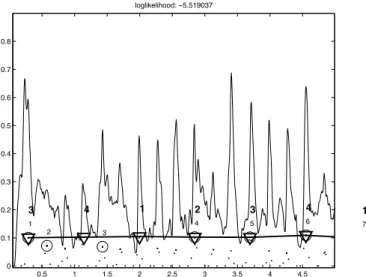
represent the downbeat locations. In Figure 2, we illustrate the results of this decoding algorithm on a real signal.

III. INITIAL PROBABILITY

The initial probability pinit(si,j) = pinit(ti 2 { j})

represent the probability to be in hidden state [time ti is a

beat and is in a specific j] at the beginning of the decoding.

We do not favor any j in particular, but we favor ti to be a

time close to the beginning of the track. pinit(si,j) is modeled

as a Gaussian function with µ = 0, = 0.5 evaluated on the

ti of all the states.

IV. EMISSION PROBABILITIES

The emission probability pobs(o(t)|si,j) = pobs(o(t)|ti 2

{ j}) represents the probability to observe o(t) given [time

3_{It should be noted that in [14], Ellis also faced this problem in its Dynamic}

0.5 1 1.5 2 2.5 3 3.5 4 4.5 0 0.1 0.2 0.3 0.4 0.5 0.6 0.7 0.8 3 4 1 2 3 4 ₁ 1 2 3 4 5 6 ₇ loglikelihood: −5.519037

Fig. 2. Viterbi decoding and backtracking: onset-energy-function (continuous thin line), states si,jand associated observation probability (dots), maximum

observation probability of each bnk(O sign), best path (continuous thick line

and 4 sign), bnk(normal number), (bold number). Signal=”Aerosmith

-Cryin”.

ti is a beat and is in a specific j]. As explained above, this

probability has a non-null emission probability only when t =

ti. This probability is computed using4:

pobs(ti2 { j}|o(t)) = pobs(t = ti) · pobs(ti2 { }|o1(t))

· pobs(ti2 { j}|o2(t), o3(t))

(3) In this, we have subdivided o(t)) as three observation

vectors o1(t)), o2(t) and o3(t). We now explain the two terms

in parts IV-A and IV-B.

A. Beat observation probabilities pobs(ti 2 { }|o1(t))

pobs(ti 2 { }|o1(t)) represents the probability to observe

[time ti is a beat] given the observation o1 at time t. As

explained above, t must be equal to ti. We therefore use the ti

notation in the following. As in many works, this probability is estimated by computing the correlation between - a

beat-template g(t) chosen to correspond to the local tempo Tb(ti)

and - the local onset-energy function starting at time ti. The

beat-template g(t) can be a simple function with values of 1 at the expected beat-position and 0 otherwise (as used in [33]). In [31], we have proposed the use of machine learning to find the beat-template that maximizes the discrimination

between the correlation values obtained when ti 2 { } and

when ti 2 { }. We summarize it here using our framework/

notations and refer the reader to [31] for details and evaluation of it.

1) Learning the best beat-template by Linear Discriminant

Analysis: We note fi(t) = f(t, t 2 [ti, ti+ 4Tb]) the values

of the local onset-energy function starting at time ti. The

beat-template g(t) must be chosen such as (a) to have the

4_{In order to split p}

obs(ti2 { j}|o(t)) in two terms we use the assumption

that o1 and o2, o3 are independent, and that o1 and o2, o3are independent

conditionally to ti 2 { j}, i.e. knowing ti2 { j}, the knowledge of o1

does not bring information on o2, o3.

1 1.5 2 2.5 3 3.5 4 4.5 5 −0.2 −0.1 0 0.1 0.2 0.3 0.4 0.5 0.6 Normalized Time

Fig. 3. Average value F (n) for the RWC-Popular-Music test-set (thick line), LDA-trained beat-template g(n) (thick line)

maximum correlation with fi(t) when ti2 { }, (b) to provide

the largest discrimination between the correlation values when

ti 2 { } and when ti 2 { }. The condition (b) is needed/

in our case since the values of correlation will be used as observation probabilities in our framework. In the following, we only discuss the case of a “binary subdivision of the beat” and “binary grouping of the beat into bar”. Extension to other meters is straightforward.

We note g(1) . . . g(N) the discrete sequence of values of the beat-template g(t) representing a one-bar duration. Considering a 4/4 meter, g(1) represents the value of at the

downbeat position, g(1 +kN

4 ) with k 2 [0, 1, 2, 3] the values

at the beat positions. In the same way, we define Fi(n) as

the function obtained by sampling the local values of fi(t) by

N value: Fi(1) = fi(ti) . . . Fi(N) = fi(ti+ 4Tb). If ti is a

beat-position, Fi(1 + kN₄ ) with k 2 [0, 1, 2, 3] represent the

values at the beat positions.

The correlation between g(n) and Fi(n) can be written as

(neglecting the normalization terms): ci(j) = PN_n=1Fi(n +

j)g(n)

If we choose ti as a beat-position, we therefore look for the

beat-template (the values of g(n), n 2 [1, N]) for which

• (a) ci(j) is maximum at j 2 [0,N₄,2N₄ ,3N₄ ]

• (b) ci(j) is minimum for all the other values of j

The problem of finding the best values of g(n) is close to the problem of finding the best weights to apply to the dimensions of multi-dimensional observations in order to maximize class separation. This problem can be solved using Linear Discrimi-nant Analysis (LDA) [36]. In our case the weights are the g(n), the dimensions of the observations are the successive values

of Fi(n)5 and the two classes are “beat” and “non-beat”. We

therefore apply a two-class Linear Discriminant Analysis to our problem.

Creating observations for the two-class LDA problem: In order to apply the Linear Discriminant Analysis, we create observations for the two classes “beat” and “non-beat”. These observations are coming from a test-set annotated into beat and downbeat positions. We create for each track l of the test-set and for each annotated bar m of a track, the corresponding

Fi,l,m(n). We then compute the vector Fi,l(n) by averaging

the values of Fi,l,m(n) over all bars of a track. By shifting

(circular permutation is assumed in the following) Fi,l(n),

5_{It should be noted that considering the values of F}

i(n)as points in a

multi-dimensional features space has been also used in [37] in the framework of rhythm classification.

we create two sets of observations corresponding to the two classes “beat” and “non-beat”: - “beat” class: the four patterns

Fb

l(n) = Fi,l(n + j) with j 2 [0,N₄,2N₄ ,3N₄ ], -

“non-beat” class: all the remaining patterns Fnb

l (n) = Fi,l(n + j) with j 2 [1, N] j /2 [0,N 4, 2N 4 , 3N

4 ]. We then apply Linear

Discriminant Analysis considering the two set of observations

Flb(n) and Flnb(n) and their associated classes “beat” and

“non-beat”.

Linear Discriminant Analysis: We compute the matrix

U such that after transformation of the multi-dimensional

observation by this matrix, the ratio of the Between-Class-Inertia and the Total-Between-Class-Inertia is maximized. If we note u the column vectors of U, this maximization leads to the condition

T 1Bu = u, where T is the Total-Inertia matrix and B

the Between-Class-Inertia matrix. The column vectors of U

are then given by the eigen vectors of the matrix T 1_B

associated to the eigen values . Since our problem is a two-classes problem, only one column remains in U. This column gives us the weights to apply to F (n) in order to obtain the best separation between the classes “beat” and “non-beat”. It therefore defines the best beat-template g(n).

Result: In Figure 3, we illustrate this for the RWC-Popular-Music test-set [38]. The thin line represents the aver-age (over the 100 tracks) vector F (n), the thick line represents the values of g(n) obtained by Linear Discriminant Analysis. As one can see, the LDA-trained beat-template assigns - large positive weights at the beat-positions (1, 2, 3, 4) and - negative weights at the counter-beat positions (1.5, 2.5, . . . ) and at the just-before/ just-after beat positions. The use of negative weights is a major difference with the weights used in usual beat-templates (as in [33]) which only use positive or zero weights. The specific locations of the negative weights allow reducing the common counter-beat detection errors (negative weights at the counter-beat positions) and the precision of the beat location (negative weights at the just-before/ just-after beat positions). This wouldn’t be achieved by using a model where all the positions outside the main beats are set to a constant negative number.

Use of the LDA-trained templates: In the beat-tracking process, the LDA-trained beat-templates g(n) are used to create the beat-templates corresponding to the local

tempo Tb(ti). For this, g(n) is considered as representing the

interval [0, 4Tb(ti)] and is interpolated to provide the values

corresponding to the sampling rate of f(t): 172 Hz. In order to save computation time, the values of gTb(t) for all possible tempo Tb can be stored in a table.

For the evaluation of beat and downbeat-tracking algorithms of part VI-C, we will use a beat-template derived from an LDA-training on the “PopRock extract” test-set. It has then been manually modified to keep only the salient points. It is represented on the right part of Figure 4 in comparison with the “simple” (as used in [33]) beat-template in the left part.

2) Optimization considerations: As mentioned above, the hidden states are defined as t 2 { }. For this, the time axis

of a music track is discretized into ti = iQ i 2 [0,T_Q] with

Q = 0.05ms. Large values of Q allows decreasing the number of hidden states but however decrease the temporal-precision of the beat-tracking. Because of that, we reassign the time

0 0.2 0.4 0.6 0.8 1 1.2 1.4 1.6 1.8 2 0 0.5 1 1.5 2 2.5 0 0.2 0.4 0.6 0.8 1 1.2 1.4 1.6 1.8 2 −0.2 −0.1 0 0.1 0.2 0.3 0.4 0.5

Fig. 4. Beat-templates used for the computation of the observation probability for a tempo of 120bpm (beat period of 0.5s) and a binary subdivision and grouping of the beat [LEFT]: Simple beat template (as used in [33]) [RIGHT]: LDA trained beat-template.

ti of the state si,j to the position around ti which leads to

the maximum correlation between the local signal f(t, t 2

[ti, ti+ 4Tb]) and the beat-template g(t). The horizon over

which the maximum correlation is searched for is proportional

to the local tempo Tb(ti) and defined by L = Tb(ti)/32.

B. BPIM observation probabilities pobs(ti2 { j}|o2, o3(t))

pobs(ti 2 { j}|o2(t), o3(t)) represents the probability to

observe [time ti is a j] given the observation o2, o3 at time

t. Any probability derived from signal observations (such as based on harmonic, spectral or loudness/ silence variation) that

allows distinguishing between the various jcan be used for it.

We use here two assumptions to derive the “bpim probability”. Each assumption is coupled with a characteristic which is coupled with a signal observation. The first one is based on the chord-change / harmonic-variation / chroma-vector-variation triplet. The second one is based on the rhythm-pattern / low-high-frequency alternance / spectral-distribution triplet. This

probability is computed using6_:

pobs(ti 2 { j}|o2(ti), o3(ti)) = pobs(ti2 { j}|o2(ti))

· pobs(ti2 { j}|o3(ti)) (4)

In this,

• pobs(ti2 { j}|o2(ti)) is the probability to observe [time

ti is a j] given the observation of chroma vectors

variation.

• pobs(ti2 { j}|o3(ti)) is the probability to observe [time

ti is a j] given the observation of spectral distribution.

1) BPIM probability based on chroma variation: The as-sumption we use is that chords are more likely to change

between 4 and 1 for a 4/4 meter. [4] or [32] also used this

assumption for downbeat estimation. We use it here to derive

the probability of all j at all times ti. The characteristics

implied by this assumption is that, if ti is a 1, the harmonic

content on its left and on its right should be different. The observation we use to highlight this, is the variation of chroma vectors over time. A large variation indicates a potential

change in harmony at time ti hence a higher probability to

6_{In order to split p}

obs(ti 2 { j}|o2o3) in two terms we use the

assumption that o2and o3are independent, and that o2and o3are independent

conditionally to ti 2 { j}, i.e. knowing ti 2 { j}, the knowledge of o3

observe a downbeat at tihence a 1. The probabilities for the

other j=2,3,4 are derived in the same way.

Chroma vector computation: The chroma vectors (or Pitch-Class-Profile vectors) [39] are computed as in [40], i.e. the Short Time Fourier Transform is first computed with a Blackman analysis window of length 0.1856ms and a hop size of 0.0309ms. Each bin is then converted to a note-scale. Median-filtering is applied to each note-band in order to reduce transients and noise. Note-bands are then grouped into 12-dimensions vectors. We note C(l, t) the values of the

l2 [1, 12] dimension of the chroma vector at time t.

Chroma vector variation: We compare the values taken

by C(l, t) on the left of tiand on its right using two temporal

window of duration ↵. We note Li,1 = [ti ↵Tb, ti] the

left window and Ri,1 = [ti, ti+ ↵Tb] the right window. ↵

is expressed as a multiple of the local beat duration. In the experiment of part VI, we will compare the results obtained with ↵ = 2 (assumption that chords change twice per measure) and ↵ = 4 (once per measure).

Sliding-window method: In the same way, we compute

pobs(ti2 { j}|o2(ti)) (the probability that tiis the jth bpim),

using the assumption that the harmonic content should be

different on the left of ti (j 1)Tb and on its right. This is

illustrated in the left part of Figure 5 for the case of a 4/4 meter

(j = 1, 2, 3, 4). The computation of pobs(ti 2 { j}|o2(ti)) is

therefore obtained by comparing C(l, t) on the intervals Li,j

and Ri,j defined by

• Li,j= [ti (↵ + (j 1))Tb, ti (j 1)Tb],

• Ri,j= [ti (j 1)Tb, ti+ (↵ (j 1))Tb].

We name this method “sliding-window method” since we slide

the analyzed signal according to our j assumption.

Distance measures: We study two measures for the

computation of the chroma vectors variation. The first measure

is the symmetrized Mahalanobis distance: d(Li,j, Ri,j) =

1

2((µ2 µ1)

T_⌃ 1

1 (µ2 µ1) + (µ1 µ2)T⌃21(µ1 µ2))

where µ1 and µ2 (⌃1 and ⌃2) are the 12-dim mean vectors

(12x12dim diagonal covariance matrixes) of the values of

C(l, t 2 Li,j) and C(l, t 2 Ri,j) respectively. The second

measure is a simple “1-cosine” distance using the vectors µ₁

and µ₂ (it has value of 1 when µ₁ and µ₂ are in orthogonal

directions): d(Li,j, Ri,j) = 1

µ₁·µ₂

||µ₁||||µ₂||. In the experiment of part VI, we will compare both distances.

BPIM probabilities: Both distances have large values

when Li,j and Ri,j have different harmonic content which

indicates a potential downbeat. We therefore use the distances

d(Li,j, Ri,j) has probabilities. For this the probabilities are

normalized: pobs(ti2 { j}|o2(ti)) = 1 P jd(Li,j, Ri,j) d(Li,j, Ri,j) (5)

In Figure 6, we illustrate the computation of pobs(ti 2

{ j}|o2(ti)) on a real signal using ↵ = 2 and a “1-cosine”

distance.

2) BPIM probability based on spectral distribution: The assumption we use is that many music tracks in popular music (pop, rock, electro) use rhythm patterns alternating

the presence of kick on 1,3 and snare on 2,4. [3] or [7]

t i -aL aL -(a+1)L (a-1)L -(a+2)L (a-2)L -(a+3)L (a-3)L p obs (t in B j | o 2 (t)) p obs (t in B 1 | o 2 (t)) p obs (t in B 2 | o 2 (t)) p obs (t in B 3 | o 2 (t)) p obs (t in B 4 | o 2 (t)) bn k-1 bn k B 1 B 2 B 3 B 4 B 1 B 2 B 3 B 4 p trans (B j' | B j )

Fig. 5. [LEFT] Computation of observation probabilities for the bpim from chromagram observation. [RIGHT] Transition probabilities between bpim.

Time [sec] Chroma dim 2 4 6 8 10 12 14 16 18 0 5 10 15 20 25 30 35 0.2 0.4 0.6 0.8 1 Time [sec]

Observation prob of bpim

2 4 6 8 10 12 14 16 18 0.5 1 1.5 2 2.5 3 3.5 4 4.5 0.1 0.2 0.3 0.4 0.5

Fig. 6. [TOP] 12-dim chromagram over time, [BOTTOM] pobs(ti 2

{ j}|o2(ti))for j = 1, 2, 3, 4 , on signal= “All Saints - Pure Shores”

from test-set “PopRock extract”.

also used this assumption. The characteristics implied by this assumption is that the spectral energy distribution will

concentrate on lower frequencies for 1,3 than for 2,4. The

observation we use to highlight this, is the relative spectral balance between high and low energy content.

Spectral balance computation: At each time ti, we

compute the ratio of the high frequency to the low frequency

energy content. For this we use a window centered on ti of

length L and a cutting frequency kmax:

r(ti) = Pti+L/2 t=ti L/2 PN/2 k=kmax|S(!k, t)|2 Pti+L/2 t=ti L/2 Pkmax k=1 P k|S(!k, t)|2 (6) where N is the number of bins of the Short Time Fourier Transform. L was chosen experimentally to Tb/2 and kmax to correspond to 150Hz.

Example: Using the “PopRock extract” test-set annotated

into beat and downbeat, we have measured the values of r(ti)

for ti2 { j=1,2,3,4}. For 135 over the 156 titles of this test-set,

r(ti) is larger for the 2/ 4 than for the 1/ 3. We therefore

use it to create a probability to observe = 1, 3 or = 2, 4.

BPIM probability: As for the chroma-variation-measure,

we use a sliding-window method to derive r(ti) for all j. At

each time ti, we compute the four values:

rj is then normalized over the j to sum unit. If ti 2 1, the

following sequence of rj will be observed [r1=low, r2=high,

r3=low, r4=high]. Since we would like the probability to have

high values for 1, low values for 2, . . . we take the negative

of rj(ti) as probability:

pobs(ti2 { j}|o3(ti)) = 1 rj(ti) (8)

In Figure 7, we illustrate the computation of pobs(ti 2

{ j}|o3(ti)) on a real signal. The left parts of each figure

represent the spectrogram of the signal and super-imposed to

it the four regions used for the computation: ti+ [ L₂,L₂],

ti Tb+[ L₂,L₂], ti 2Tb+[ L₂,L₂] and ti 3Tb+[ L₂,L₂].

We also indicate the cutting frequency of 150Hz. The right

part of each figure indicates the four values of pobs(ti 2

{ j}|o3(ti)) at the given position. The upper figure represents

the values obtained when ti is a 1, the lower one a 2.

Time [sec] Frequency [Hz] 0.5 1 1.5 2 2.5 3 0 100 200 300 400 500 600 700 800 900 1000 1 2 3 4 0 0.1 0.2 0.3 0.4 0.5 0.6 0.7 0.8 0.9 1 bpim p(bpim|o(t)) Time [sec] Frequency [Hz] 1 1.5 2 2.5 3 3.5 0 100 200 300 400 500 600 700 800 900 1000 1 2 3 4 0 0.1 0.2 0.3 0.4 0.5 0.6 0.7 0.8 0.9 1 bpim p(bpim|o(t))

Fig. 7. [TOP] Spectrogram and pobs(ti2 { j}|o3(ti))for j = 1, 2, 3, 4

for ti on a 1, [BOTTOM] Spectrogram and pobs(ti 2 { j}|o3(ti))for

j = 1, 2, 3, 4for tion a 2 on signal= “Aerosmith - Walk This Way” from

test-set “PopRock extract”.

V. TRANSITION PROBABILITIES

The transition probability ptrans(ti0 2 { j0}|ti 2 { j})

represents the probability to transit from [time ti is a beat and

is in a specific j] to [time ti0 is a beat and is in a specific

j0]. We compute it using:

ptrans(ti0 2 { j0}|ti 2 { j}) = ptrans(ti0 2 { }|ti2 { })· ptrans(ti0 2 { j0}|ti2 { j})

(9) We also add the condition that only transition to increasing

times ti (increasing states si,j) are allowed. This makes our

model a Left-Right HMM. A. Beat transition probabilities

ptrans(ti0 2 { }|ti 2 { }) represents the fact that the

successive times ti associated to the beats must have an

inter-distance close to the local tempo period Tb(ti). The transition

probability models the tolerated departure from this period.

We have used a Gaussian function with µ = Tb(ti), = 0.05s

evaluated at = ti0 ti.

B. BPIM transition probabilities

ptrans(ti0 2 { j0}|ti 2 { j}) represents the probability

to transit from a beat in j to a beat in j0. This transition

probability constrains the j to follow the circular permutation

specific to the considered musical meter: 1 ! 2 ! 3 ! 4 ! 1 ! . . . for a 4/4 meter; 1 ! 2 ! 3 ! 1 . . . for a 3/4 meter. As proposed in [34], a generic formulation of the transition matrix allowing potential meter changes between 4/4 and 3/4 meters over time can be written as

Mtrans(bnk 1, bnk) = 0 B B @ 0 1 0 0 0 0 1 0 ↵ 0 0 1 1 ↵ 0 0 0 1 C C A (10)

where bnk is the beat-number used for the decoding axis and

↵_{2 [0, 1] is a coefficient favoring meter changes (↵ > 0) or}

constant-4/4-meter-over-time (↵ = 0). In the experiments done so far, we have obtained better results using ↵ = 0 (constant-4/4-meter-over-time). In the experiment of part VI, we will therefore only consider the case ↵ = 0 (constant-4/4-meter-over-time). The corresponding matrix is illustrated in the right part of Figure 5.

VI. EVALUATION

In this part, we evaluate the performance of the proposed algorithm for beat and downbeat-tracking using various con-figurations. We compare them to the results obtained with our previous systems and to the results obtained to state-of-the-art results. It should be noted that the evaluation performed here only concerns the quality of beat and downbeat-tracking algorithms. However, because the input of our system are the time-variable tempo and meter estimations coming from the algorithm of [29], the results obtained also depend on the quality of the estimation of those.

A. Evaluation rules

Over the years, a large number of measures have been proposed to estimate the performances of beat-tracking algo-rithms: F-measure of Dixon [5], Gaussian error function of Cemgil [41], set of boolean decisions of Goto [42], perceptual P-score of McKinney [43], continuity based measures CMLc, CMLt, AMLc, AMLt of Goto [42], Hainsworth [44] and Klapuri [7], information based criteria based of Davies [19]. We refer the reader to [19] or to the set of rules used for the MIREX-09 “Audio Beat Tracking” contest [22] for a good and detailed overview of those.

In this evaluation, we indicate the results using two

cri-teria7_{. The first is the F-measure for a relative-tempo-length}

Precision Window of 0.1. We use it for beat and downbeat evaluation when comparing the performances of the various configurations of our system. The second is the set of CMLc, CMLt, AMLc and AMLt criteria. We use them in order to be

7_{The results of the experiments using the other criteria (using}

Dixon, Cemgil, Goto, McKinney . . . criteria) can be found at the

following URL http:// recherche.ircam.fr/ equipes/

able to compare our results to the ones published in previous works on the same test-sets.

F-measure at a relative-tempo-length Precision Window of 0.1: Considering a given beat/ downbeat marker annotation and a given track, we note - A: the number of annotated beats (downbeats), - D: the number of detected ones and - CD(PW): the number of correctly detected ones within a given Precision Window (PW). From this we derive the following measures:

• Recall(P W ) = CD(P W )_A ,

• P recision(P W ) = CD(P W )_D ,

• F M easure(P W ) = 2R(P W )_{R(P W )+P (P W )}·P (P W ).

Note that the Precision Window is centered on the annotated beat (downbeats) for the Recall and on the estimated beat for the Precision.

Octave errors: Using this measure, we do not consider

octave errors as correct8_{. For a correct beat marking but at}

twice (three time) the tempo, the Recall will be 1 but the Precision 0.5 (0.33). for a correct beat marking at half (one third of) the tempo, the Precision will be 1 but the Recall 0.5 (0.33).

Adaptive Precision Window: In our evaluation the Precision Window is defined as a percentage of the local annotated beat length Tb. This is done in order to avoid drawing misleading

conclusions from the results9_{. PW=↵ means that the estimated}

beat should be at a maximum distance of ±↵Tb the annotated beat. For a given track, we consider the minimum value of

Tb(ti) over time (the fastest annotated tempo). The values

given in the following correspond to the average (over all tracks of a test-set) of the F-measure(PW=0.1).

Statistical hypothesis tests: Considering that the values given in the evaluation are only estimates of the average F-measure, we also perform statistical tests (pair wise Student T-tests) in order to infer the statistical significances of the

difference of values. We use a 10% significance level10_.

CMLc, CMLt, AMLc and AMLt: When comparing our results to previously published results we will use the follow-ing measures: - CMLc (Correct Metrical Level with continuity required), - CMLt (same but no continuity required), - AMLc (All Metrical Level with continuity required) and - AMLt (same but no continuity required). We refer the reader to [42] [44] and [7] for more details. For the implementation of CMLc, CMLt, AMLc and AMLt we have used the

imple-mentation kindly provided by M. Davies11_{. These measures}

correspond to the “Correct” and “Accept d/h” criteria and the “Continuity required” and “Individual estimate” categories

8_{This is because the usual halving or doubling of the tempo is actually}

only correct for a binary simple meter. For most test-sets we do not have information about the grouping/subdivision of the beats/ tactus (by two or three). Moreover, in the case of beat-tracking, - doubling the tempo will require to check that the detected markers correspond to all the tatum (and not only the counter-beat ones), - halving the tempo will require to check that the detected markers corresponds to the dominant beats (downbeats) in the measure.

9_{Indeed a fixed PW of 0.166s would be restrictive for slow tempi (half-beat}

duration of 0.5 at 60bpm) but will mean accepting counter-beat as correct for fast tempi (half-beat duration of 0.166s at 180bpm).

10_{The choice of 10%, instead of the usual 5%, has been made to better}

emphasizes the differences between algorithms.

11_{The evalbeat toolbox is accessible at http:// www.elec.qmul.ac.uk/}

digi-talmusic/ downloads/ beateval/ beateval.zip

used in [7]. A precision window of 17.5% as in [7] is used for both estimated marker position and estimated tempo. B. Test-sets

For the evaluation, we have used six test-sets.

T-PR: The “PopRock extract” is a collection of 155 major top-ten hits of the past decades. Only 20s extract of the tracks are considered. The annotations into beat and downbeat have been made by one of the authors.

T-RWC-P: The “RWC Popular Music” [45] is a collection of 100 tracks in full-duration of Pop-rock-ballad-heavy-metal popular music.

T-RWC-J: The “RWC Jazz Music” [45] is a collection of 50 tracks in full-duration of Jazz-music with solo piano, guitar, small ensemble or modern-jazz orchestra. The difficulty of this test-set comes from the complexity of the rhythms used in Jazz-music.

T-RWC-C: The “RWC Classical Music” [45] is a collection of 59 tracks in full-duration of Classical-music. The difficulty of this test-set comes from the tempo variations used in Classical-music. The annotations of the three RWC test-sets are provided by the AIST [46].

T-KLA: “Klapuri” test-set is the one used in [7]. It contains 505 tracks of a wide range of music genre (pop, metal, electro, classical). 474 of them are annotated in beat positions for an excerpt in the middle of the track. Because only beat-phase annotations are provided we do not evaluate downbeat-tracking here.

T-HAI: “Hainsworth” test-set is the one used in [12], [8] and [47]. It contains 222 tracks, each around 60s length from a large variety of music genres and with time-variable tempo. Because only beat-phase annotations are provided we do not evaluate downbeat-tracking here. It should be noted that only the values of Davies “Detection Function” DF are provided (not the audio signal). The DF function has a sampling rate of 86.2Hz (step of 11.6ms). Therefore we have modified our system in order to use the DF function instead of our reassigned-spectral-energy-flux (RSEF) function. This concerns both our tempo/ meter estimation and beat-tracking algorithms. We therefore test the generalization of the LDA-trained beat-templates when applied to other functions than the one (the RSEF function) used for training.

The T-PR, and the RWC test-sets have been used since they are annotated in beat and downbeat positions. The three RWC test-sets are also available to the research community for

comparison. The T-KLA and T-HAI12_{have been used in order}

to provide a comparison with state-of-the-art published results. We also present the results obtained during the MIREX-09 evaluation which use other test-sets.

C. Beat and Downbeat-tracking results and discussion In this part, we evaluate the performances of various config-urations of our beat and downbeat-tracking algorithm. Table I indicates the results in terms of F-measure with a Precision

12_{We are grateful to A. Klapuri, St. Hainsworth and M. Davies to have let}

Window of 0.1 for T-PR, T-RWC-P, T-RWC-J and T-RWC-C using the following configurations:

• “P-sola” are the results obtained with the P-sola

beat-tracking algorithm [31] (no downbeat estimation is avail-able for this algorithm).

• “Viterbi” refers to the model proposed in this paper.

• “Viterbi no-DB” refer to the reduced model without

estimating the downbeat and j (we only use pobs(ti 2

{ }|o1))

• “Viterbi DB” refer to the full model including downbeat

estimation (we use pobs(ti2 { j}|o1, o2, o3))

• “Simple/ LDA” refers to the use of the corresponding

beat-template in the computation of pobs(ti2 { }|o1).

• “↵ = 4 / ↵ = 2” refers to the duration of the window

used for the computation of pobs(ti2 { j}|o2(t)).

• “COS/ MAH” refers to the use of the “1-cosine” or

“Mahalanobis” distance for the computation of pobs(ti2

{ j}|o2(t)).

• “CHRO” refers to the use of observation probability

based on chroma variation (pobs(ti2 { j}|o2))

• “SPEC” refers to the use of observation probability based

on spectral distribution (pobs(ti 2 { j}|o3)). Note that

we do not provide the results using “SPEC” alone since

the use of pobs(ti2 { j}|o3) alone did not lead to good

results.

• “Chord Detection” refers to the results obtained using the

downbeat estimation obtained using the chord estimation algorithm of [32]. In this case, the input of the system is the best beat estimation (“Viterbi no-DB LDA”). As mentioned in part IV-A1 the LDA-trained beat-template used in all the experiments here is a beat-template manually derived from an LDA-training on T-PR (see Figure 4). It should be noted also that when using the Viterbi algorithm, both beat and downbeat estimation are obtained at the same time.

TABLE I

Beat and Downbeat estimation results for T-PR, T-RWC-P, T-RWC-J and T-RWC-C.

P-sola against Viterbi: We first compare the P-sola to the Viterbi beat-tracking algorithm. For this we use the base-line Viterbi algorithm, i.e. using the “Simple” beat-template.

Results shows a large improvement of the F-measure(PW=0.1) for all test-sets except for T-RWC-C. This difference is statis-tically significant for T-PR, T-RWC-P and T-RWC-J.

Choice of the beat-template (LDA or Simple): We then compare the use of a “Simple” (as used in [33]) to the LDA-trained template. The use of the LDA-trained beat-template leads to a small improvement of beat-tracking results for 2 over 4 test-sets: from FMeas=0.91 to 0.93 for T-PR, 0.4 to 0.42 for T-RWC-C. Remark that the largest improvement is obtained on T-PR which is the test-set used to train the LDA-trained beat template. There is however no statistical significance for these 2 test-sets. We will show in the following that for T-KLA and T-HAI (which are larger test-sets), there is a statistically significant difference between the “Simple” and LDA-trained beat-templates.

We now evaluate the results of downbeat-tracking.

Best parameters for BPIM probability based on chroma variation: For 3 over 4 test-sets, the use of a window duration of ↵ = 2 (making the assumption that chords change twice per measure) leads to better results than ↵ = 4 (chords change once per measure): FMeas=0.68 and 0.53 for T-PR, 0.76 and 0.78 for T-RWC-P, 0.46 and 0.40 for T-RWC-J, 0.35 and 0.23 for T-RWC-C. This difference is statistically significant for T-PR and T-RWC-C.

For all test-sets, the use of the “1-cosine” distance leads to better results than the use of the symmetrized Mahalanobis distance: FMeas=0.68 and 0.44 for T-PR, 0.76 and 0.49 for RWC-P, 0.46 and 0.31 for RWC-J, 0.35 and 0.23 for T-RWC-C. This difference is statistically significant for the four test-sets. This result is surprising since the “1-cosine” distance does not take into account the inherent chroma variation inside

Li,j and Ri,j. The bad results obtained with the Mahalanobis

distance may be explained by the fact that Li,j and Ri,j are

too short to reliably estimate the covariance matrices. Using simultaneously BPIM probability based on chroma variation and spectral balance: For 3 over 4 test-sets, the inclusion of the BPIM probability based on “spectral balance” allows to further increase the results: from FMeas=0.68 to 0.74 for T-PR, 0.76 to 0.8 for T-RWC-P, 0.46 to 0.47 for T-RWC-J, 0.35 to 0.34 for T-RWC-C. The increase is larger when the file duration is short (T-PR). This can be explained by the fact that BPIM probability based on chroma variation necessitates long duration observation which is not the case of BPIM probability based on spectral balance. Hence a large increase for short duration files. The increase also mainly occurs for files belonging to the Pop and Rock music genre. This can be explained by the fact that BPIM probability based on “spectral balance” makes the underlying assumption of a “kick/ snare/ kick/ snare” rhythm pattern, which does not exist in Jazz and Classical music. However there is no statistical significance for none of the test-set.

Downbeat estimation (Viterbi against Chord detection): We finally compare the results obtained with our complete system (Viterbi DB LDA a=2 COS CHRO/SPEC) to the results obtained using the “Chord detection” algorithm of [32]. For 3 over 4 test-sets, the proposed algorithm allows to improve the downbeat-tracking results: FMeas=0.74 and 0.64 for T-PR, 0.8 and 0.81 for T-RWC-P, 0.47 and 0.44 for T-RWC-J,

0.34 and 0.32 for T-RWC-C. Only for T-PR, this difference is statistically significant.

Variations among test-set: As one can observe, the perfor-mances of beat-marking are best for the T-PR (FMeas=0.93) and T-RWC-P (0.84) than for the more complex Jazz rhythm of T-RWC-J (0.57) or the time-variable tempo of Classical music of T-RWC-C (0.42). The same can be observed for the downbeat marking (0.74, 0.8, 0.47, 0.34).

D. Comparison to other works

1) Evaluation using Klapuri [7] test-set: In Table II, we compare the results of our Viterbi algorithm using “simple” or “LDA-trained” beat-templates to the results published in [7] using the test-set used in [7]. The LDA-trained templates achieved higher results than the “simple” beat-template: FMeas=0.64 and 0.67. This difference is statistically significant. For the criteria for which temporal continuity is not required (CMLt and AMLt), the performances of our Viterbi-LDA algorithm are higher than that of [7]: from CMLt= 64 to 65, from AMLt= 80 to 83. This improvement is however small. For the criteria for which temporal continuity is required (CMLc and AMLc), the performances of our algorithm are lower than that of [7].

TABLE II

Beat estimation results for T-KLA [7] and T-HAI [12] test-set.

2) Evaluation using Hainsworth [12] test-set: In Table II, we compare the results of our Viterbi algorithm using “simple” or “LDA-trained” beat-templates to the recent results published in Stark [47] using the test-set used in [12], [8] and [47]. “Klapuri et al. (NC)” refers to the non-causal algorithm of [7], “Davies and Plumbley (NC)” refers to the non-causal algorithm of [8] and “SDP + 1stbeat + Tempo” refers to the results obtained with the Stark et al. algorithm [47] using annotated tempo and annotated first beat-phase. Again, for this test-set, the LDA-trained beat-templates achieved higher results than the “simple” beat-template: FMeas=0.56 and 0.63. This difference is again statistically significant. This is an important results since the input of our system was in this case Davies “Detection Function” DF and not our reassigned-spectral-energy-flux (RSEF) function which was used for the training of the LDA-beat templates. This somehow proofs the generalibity of the proposed LDA-trained beat templates. For the criteria for which octave errors are considered corrects (AMLc and AMLt), the performances of our Viterbi-LDA algorithm are higher than all the other algorithms: AMLc=70.8 and AMLt=81.8. For the criteria for which octave errors are

not considered corrects (CMLc and CMLt), the performances of our algorithm are lower than that of the other algorithms. These results could indicate that our tempo estimation system suffers from many octave errors. However, this results must be taken with care since we did not have access to the audio data but only to the values of the DF function. Because, the

DF function has different properties than our RSEF function,

it may not fit completely the shape of the templates (see [29]) used for our tempo/ meter estimation.

3) MIREX Audio Beat Tracking Contest results: We have submitted our tempo and beat-marking system to the MIREX-09 Audio Tempo Extraction contest [22]. For this evaluation, we tested four configuration of the tempo estimation stage of [29] (variable-over-time or constant-over-time tempo estimation, meter estimated or forced to 4/4) but only one of the beat marking stage (corresponding to Viterbi DB LDA COS CHRO). Two test-sets were used: the “McKinney Collection” and the “Sapp’s Mazurka Collection”. The “McKinney Collection” is a set of 160 musical excerpts; each recording has been annotated by 40 different listeners (39 in a few cases) [48] [49]. The “Sapp’s Mazurka Collection” is a set of 322 files drawn from the Mazurka.org dataset put together by Craig Sapp. He was also responsible for creating the high-quality ground-truth files. The whole set of performance measures, collected by Davies, was used for the evaluation: F-Measure, Cemgil, Goto, P-score, CMLc, CMLt, AMLc, AMLt, . . . . On the “McKinney Collection” test-set, for 8 criteria over 10, our system ranked first, and this whatever configuration of the tempo estimation stage. For the two remaining criteria (AMLc and Davies D criteria), our system ranked second whatever configuration of the tempo estimation part. Since this test-set is the same as the one used in the MIREX-06 “Audio Beat Tracking” task, and since the P-score is available for both MIREX-06 and MIREX-09, we compare the largest P-score obtained in MIREX-06 to the ones we have obtained in 2009. In 2006,

Dixon reaches a P-score0.575. In 2009, our system whatever

configuration of it has a P-score from 0.579 to 0.592. On

the “Sapp’s Mazurka Collection” test-set, the best performing algorithm was the DRP3 from Davies, and this for all criteria. The best performing configuration of our system was with [variable-over-time tempo estimation, meter is estimated] which ranked 2nd for 8 criteria over 10 (except the Goto and Davies D criteria). We refer the reader to http:// www.music-ir.org/ mirex/ 2009/ index.php/

Audio_Beat_Tracking_Resultsfor more details.

VII. CONCLUSION ANDFUTURE WORKS

In this paper we have proposed a probabilistic framework for simultaneous beat and downbeat-tracking from an audio signal given estimated tempo and meter as input.

We have proposed a hidden Markov model formulation in which hidden states are defined as “time t is a beat in a specific beat-position-in-measure”. Since times are part of the hidden states definition, we have proposed a “reverse” Viterbi decoding algorithm which decodes times over beat-numbers. The beat observation probabilities are obtained by

using beat-templates. We have proposed the use of Linear Discriminant Analysis to compute the most discriminant beat-templates. We have shown that the use of this LDA-trained beat-template allows an improvement of beat-tracking results for 4 over the 6 test-sets used in our evaluation. For the “Klapuri” and “Hainsworth” test-sets, this difference is sta-tistically significant. It is important to note that “Klapuri” and “Hainsworth” test-sets are the two largest and were not part of the development of our system.

The beat-position-inside-measure (bpim) allows deriving simultaneously beat and downbeat position. We have proposed two bpim observation probabilities. The first probability is based on analyzing the variation of chroma vector over time. We have studied two window lengths for their computation (corresponding to the assumptions that chord change twice or once per measure) and two distances for their comparison (“1-cosine” and symmetrized Mahalanobis). The best results have been obtained using a window length of two beats and a “1-cosine” distance. The second probability is based on analyzing the temporal pattern of the spectral balance. The inclusion of this second probability allows increasing further the downbeat tracking results.

We have compared the results obtained by our new systems to our previous P-sola beat-tracking algorithm (as used in MIREX-05 contest) [31]. Results show a large improvement of the beat-tracking results which is statistically significant for all test-sets. We have then compared the results obtained by our new system to our previous chord-based downbeat-tracking algorithm [32]. The new algorithm allows increasing the results for 3 over 4 test-sets. For the “PopRock extract” test-set, the difference is statistically significant.

We have compared our results to the one obtained in [7] [12] [8] and [47] using the same test-sets and evaluation measures. For the “Klapuri” test-set, the proposed algorithm allows improving the results for the measures CMLt and AMLt (which do not require temporal contiguity), however this is not the case for the category CMLc and AMLc (which require temporal contiguity). Our algorithm seems therefore to suffer from temporal discontinuity. This may be due to the large

transition probability assigned to ptrans(ti0 2 { }|ti 2 B) in

our experiment. For the “Hainsworth” test-set, the proposed algorithm allows improving the results for the measures AMLc and AMLt (which consider octave errors as correct), however this is not the case for the category CMLc and CMLt (which do not consider octave errors as correct). Our algorithm seems therefore to suffer from octave errors. Finally, we have discussed the results obtained by our algorithm in the last MIREX-09 beat-tracking contest in which our algorithm ranked first for the “McKinney Collection” test-set but only ranked second for the “Mazurka” test-set.

Considering the results obtained and the adaptability to include new observation probabilities, the proposed proba-bilistic formulation is promising. The computation time and memory cost is however higher than other methods. However, the method can be highly optimized when implementing it. The C++ version of this algorithm was for example the fastest algorithm in the MIREX-09 contest. Future works will concentrate on adding new type of observations probabilities

for the bpim probability such as relative silence detection. The LDA-trained beat template used here was the one trained on the PopRock test-set. This PopRock template was applied to Jazz and Classical music. Ideally, one would choose the most appropriate LDA-trained beat-template for the music genre studied. Further work will therefore concentrate on integrating automatic music genre estimation to our system in order to choose the most appropriate beat-template. Finally, our current system is composed of two independent parts: tempo and meter estimation on one side, beat and downbeat estimation on the other side. Both parts use a hidden Markov model formulation, further work will therefore concentrate on estimating them simultaneously in the same framework as did for example Laroche in [33].

VIII. ACKNOWLEDGMENTS

This work was partly supported by “Quaero” Program funded by Oseo French State agency for innovation. Many thanks to Frederic Cornu for careful optimization and debug-ging of code and Christophe Veaux for help on probabili-ties. Many thanks to Anssi Klapuri, Stephen Hainsworth and Matthew Davies for sharing their test-set and the beat-tracking evaluation toolbox.

REFERENCES

[1] F. Gouyon and S. Dixon, “A review of rhythm description systems,” Computer Music Journal, vol. 29, no. 1, pp. 34–54, 2005.

[2] A. Marsden, Journal of New Music Research: Special Issue on Beat and Tempo Extraction, 2007.

[3] M. Goto and Y. Muraoka, “Music understanding at the beat level real-time beat tracking for audio signals,” in Proc. of IJCAI (Int. Joint Conf. on AI) / Workshop on CASA, 1995, pp. 68–75.

[4] ——, “Real-time rhythm tracking for drumless audio signals - chord change detection for musical decisions,” in Proc. of IJCAI (Int. Joint Conf. on AI) / Workshop on CASA, 1997, pp. 135–144.

[5] S. Dixon, “Evaluation of audio beat tracking system beatroot,” Journal of New Music Research, vol. 36, no. 1, pp. 39–51, 2007.

[6] E. Scheirer, “Tempo and beat analysis of acoustic musical signals,” J. Acoust. Soc. Am., vol. 103, no. 1, pp. 588–601, 1998.

[7] A. Klapuri, A. Eronen, and J. Astola, “Analysis of the meter of acoustic musical signals,” IEEE Trans. on Audio, Speech and Language Processing, vol. 14, no. 1, pp. 342–355, 2006.

[8] M. Davies and M. Plumbley, “Context-dependent beat tracking of musical audio,” IEEE Trans on Audio, Speech and Language Processing, vol. 15, no. 3, pp. 1009–1020, 2007.

[9] M. Goto and Y. Muraoka, “Real-time beat tracking for drumless audio signals: Chord change detection for musical decisions,” Speech Commu-nication, vol. 27, pp. 311–335, 1999.

[10] T. Jehan, “Creating music by listening,” PHD Thesis, Massachusetts Institute of Technology., 2005.

[11] A. Cemgil and B. Kapen, “Monte carlo methods for tempo tracking and rhythm quantization,” Journal of Artificial Intelligence Research, vol. 18, pp. 45–81, 2003.

[12] S. Hainsworth and M. Macleod, “Beat tracking with particle filtering algorithms,” in Proc. of IEEE WASPAA, New Paltz, NY, 2003. [13] J. Laroche, “Estimating tempo, swing and beat locations in audio

recordings,” in Proc. of IEEE WASPAA, New Paltz, NY, USA, 2001. [14] D. Ellis, “Beat tracking by dynamic programming,” J. New Music

Research, vol. 6, no. Special Issue on Beat and Tempo Extraction, pp. 51–60, 2007.

[15] J. Seppanen, “Tatum grid analysis of musical signals,” in Proc. of IEEE WASPAA, New Paltz, NY, USA, 2001.

[16] F. Gouyon, “A computational approach to rhythm description,” PHD thesis, Universitat Pompeu Fabra, Barcelona, Spain, 2005.

[17] D. Eck and N. Casagrande, “Finding meter in music using an autocor-relation phase matrix and shannon entropy,” in Proc. of ISMIR, London, UK, 2005.