Pressurized groundwater outflow experiments and numerical modeling for outflow channels on Mars

HAL Id: insu-02276022

https://hal-insu.archives-ouvertes.fr/insu-02276022

Submitted on 5 Mar 2021

HAL is a multi-disciplinary open access

archive for the deposit and dissemination of

sci-entific research documents, whether they are

pub-lished or not. The documents may come from

teaching and research institutions in France or

abroad, or from public or private research centers.

L’archive ouverte pluridisciplinaire HAL, est

destinée au dépôt et à la diffusion de documents

scientifiques de niveau recherche, publiés ou non,

émanant des établissements d’enseignement et de

recherche français ou étrangers, des laboratoires

publics ou privés.

Wouter Marra, Ernst Hauber, Stuart Mclelland, Brendan Murphy, Daniel

Parsons, Susan Conway, Manuel Roda, Rob Govers, Maarten Kleinhans

To cite this version:

Wouter Marra, Ernst Hauber, Stuart Mclelland, Brendan Murphy, Daniel Parsons, et al..

Pres-surized groundwater outflow experiments and numerical modeling for outflow channels on Mars.

Journal of Geophysical Research.

Planets, Wiley-Blackwell, 2014, 119 (12), pp.2668-2693.

RESEARCH ARTICLE

10.1002/2014JE004701

Key Points:

• Different groundwater pressures result in different outflow processes • These range from seepage, fissure

flow to the eruption of subsurface reservoirs

• Such reservoirs created by flexure can explain extreme outflow events on Mars Supporting Information: • Readme • Video S1 • Video S2 • Video S3 Correspondence to: W. A. Marra, w.a.marra@uu.nl Citation:

Marra, W. A., E. Hauber, S. J. McLelland, B. J. Murphy, D. R. Parsons, S. J. Conway, M. Roda, R. Govers, and M. G. Kleinhans (2014), Pressurized groundwater outflow experiments and numerical modeling for outflow channels on Mars,

J. Geophys. Res. Planets, 119, 2668–2693,

doi:10.1002/2014JE004701.

Received 24 JUL 2014 Accepted 21 NOV 2014

Accepted article online 26 NOV 2014 Published online 23 DEC 2014

Pressurized groundwater outflow experiments and numerical

modeling for outflow channels on Mars

Wouter A. Marra1_{, Ernst Hauber}2_{, Stuart J. McLelland}3_{, Brendan J. Murphy}3_{, Daniel R. Parsons}3_,

Susan J. Conway4_{, Manuel Roda}1_{, Rob Govers}1_{, and Maarten G. Kleinhans}1

1_{Faculty of Geosciences, Universiteit Utrecht, Utrecht, Netherlands,}2_{DLR, Deutsches Zentrum für Luft- und Raumfahrt,}

Berlin, Germany,3Department of Geography Environment and Earth Sciences, University of Hull, Hull, UK,4Department of Physical Sciences, Open University, Milton Keynes, UK

Abstract

The landscape of Mars shows incised channels that often appear abruptly in the landscape, suggesting a groundwater source. However, groundwater outflow processes are unable to explain the reconstructed peak discharges of the largest outflow channels based on their morphology. Therefore, there is a disconnect between groundwater outflow processes and the resulting morphology. Using a combined approach with experiments and numerical modeling, we examine outflow processes that result from pressurized groundwater. We use a large sandbox flume, where we apply a range of groundwater pressures at the base of a layer of sediment. Our experiments show that different pressures result in distinct outflow processes and resulting morphologies. Low groundwater pressure results in seepage, forming a shallow surface lake and a channel when the lake overflows. At intermediate groundwater pressures, fissures form and groundwater flows out more rapidly. At even higher pressures, the groundwater initially collects in a subsurface reservoir that grows due to flexural deformation of the surface. When this reservoir collapses, a large volume of water is released to the surface. We numerically model the ability of these processes to produce floods on Mars and compare the results to discharge estimates based on previous morphological studies. We show that groundwater seepage and fissure outflow are insufficient to explain the formation of large outflow channels from a single event. Instead, formation of a flexure-induced subsurface reservoir and subsequent collapse generates large floods that can explain the observed morphologies of the largest outflow channels on Mars and their source areas.

1. Introduction

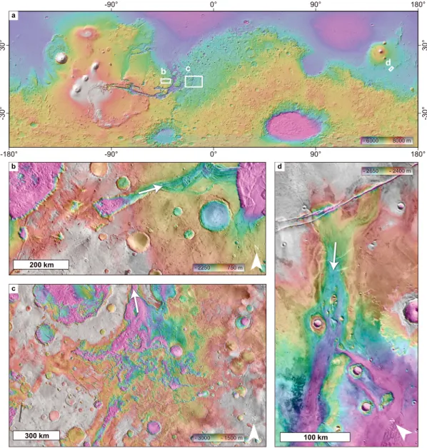
Outflow channels on Mars are among the most remarkable geomorphological features in our solar system (Figure 1). Their morphology indicates that the floods that carved them into the surface of Mars were huge, even when compared to similar reconstructions of large-scale paleofloods on Earth [Baker and Milton, 1974]. Although the fluvial processes responsible for this morphology on Mars are now generally well understood, the origin and necessary climatic conditions associated with the source areas of these channels remain a subject of debate [e.g., Harrison and Grimm, 2009, Wilson et al., 2004a]. The geomorphology, in particular the sharp transition from surrounding terrains to the source areas (Figures 1b and 1d), suggests that these channels were fed by groundwater [Baker and Milton, 1974; Sharp and Malin, 1975; Komar, 1979]. Moreover, the large depressions (Figure 1b) and chaotic terrains (Figure 1c) often found at the source of the outflow channels indicate a rather violent release of groundwater [e.g., Carr, 1979; Rodr´ıguez et al., 2005; Coleman, 2005]. However, the currently assumed groundwater outflow processes, in conjunction with the hydrological properties of the Martian crust, are thought to be unable to supply sufficient water for the largest outflow channels [Harrison and Grimm, 2009].

Catastrophic releases of vast amounts of water occurred on Earth in the past. Often-cited examples as possible analogues for the Martian outflow channels are outbursts from subglacial reservoirs or Jökulhlaups [Björnsson, 2003] and the Channeled Scabland in eastern Washington (USA) which were formed by the release of water from a breached glacial lake [Baker, 2009]. Other extreme fluvial events result from the outburst of water from reservoirs after the sudden collapse of natural or artificial dams [Waythomas et al., 1996; Major et al., 2012]. These terrestrial analogues share many morphological features with outflow channels on Mars, for example, fluvial cataracts, streamlined islands, and erosive ridges [Baker, 2009]. An interesting similarity between these terrestrial catastrophic flooding events is that they are outbursts

Figure 1. (a) Global map of Mars and (b) local maps of Ravi Vallis, (c) Iani Chaos at the source Ares Vallis, and (d)

Athabasca Vallis. Figure 1a is color-coded gridded elevation data from the Mars Orbiter Laser Altimeter (MOLA) [Zuber

et al., 1992], with shaded relief, Figures 1b–1d comprises color-coded MOLA elevation data overlain by Thermal Emission

Imaging System (THEMIS) day-time infrared mosaics [Christensen et al., 2004; Fergason et al., 2013], White arrows point downstream. Minimum and maximum elevation of linear color scale is indicated in each figure.

originating from large water reservoirs. Indeed, in several Martian cases there is also evidence that such reservoirs existed [e.g., Irwin et al., 2002; Coleman et al., 2007a; Harrison and Grimm, 2008]. However, the similarity of the fluvial morphology of these terrestrial analogues and the outflow channels on Mars contrast with the enigmatic source areas for some outflow channels. These areas often consist of chaotic terrains comprised of tilted blocks, fractures, and holes. Several theories exist on the formation of these chaotic terrains: chemical processes [Komatsu et al., 2000; Kargel et al., 2007], melt or sublimation of (subsurface) ice [Roda et al., 2014; Zegers et al., 2010; Pedersen and Head, 2011; Chapman and Tanaka, 2002; Maxwell and

Picard, 1974], and/or the release of pressurized groundwater [Carr, 1979; Rodr´ıguez et al., 2005; Wang et al.,

2005, 2006].

The scenario for pressurized groundwater outflow on Mars is based on the cryosphere model of Clifford [1993] and Clifford and Parker [2001]. In this system, an aquifer is confined underneath a cryosphere. The porous aquifer is probably a megaregolith consisting of fractured impact-ejecta and brecciated rock [Hanna

permit pressures in excess of the hydrostatic groundwater head. In this model of pressurized groundwater development, the proposed cryosphere reached a thickness of several kilometers and could thus sustain high pressures. Pressurized groundwater could have been produced via (1) infiltration from higher areas like Tharsis or the south polar ice cap [Clifford, 1993; Harrison and Grimm, 2004; Andrews-Hanna and Lewis, 2011], (2) tectonic activity or impacts [Hanna and Phillips, 2006; Wang et al., 2005], or (3) rapid freezing of the aquifer [Wang et al., 2006]. Mechanisms for the fracturing of the confining layer of frozen regolith vary from hydrofracturing produced by the groundwater pressure itself [Andrews-Hanna and Phillips, 2007], through intrusive volcanism [Russell and Head, 2003; Head et al., 2003] or preexisting tectonic features such as faults. The aquifer model developed by Hanna and Phillips [2005] provides hydrological properties to quantitatively model floods of groundwater outbursts. Harrison and Grimm [2004] showed that groundwater recharge at the high elevation of the Tharsis rise, aided by radial faults, would have been an effective mechanism to provide groundwater to the circum-Chryse outflow areas. However, an improved version of this model using more realistic permeability variations only shows limited evidence of groundwater reaching the pressures required to form the circum-Chryse outflow channels from a global-scale groundwater system [Harrison and

Grimm, 2009].

Most importantly, the currently proposed groundwater outflow models do not explain the estimated discharge based on remnant fluvial morphology [Wilson et al., 2004b] and thus suggests a poor understanding of these systems [Harrison and Grimm, 2009]. These models of groundwater outflow can only attain discharges that correspond with reconstructed estimates based on the morphology when unrealistically high values for permeability are assumed, suggesting that a more effective outflow mechanism for groundwater outflow is responsible of the formation of these channels [Head et al., 2003]. Evidence for enhanced outflow processes involving flow though fissures can be observed in the Cerberus Fossae, but this still implies very high permeability and repeated activity [Manga, 2004]. Moreover, both

Andrews-Hanna and Phillips [2007] and Harrison and Grimm [2008] show that predicted discharge through

the chaotic terrains yield relatively low discharges compared to the eroded volume, and thus, many outflow events are then required to explain the size of the outflow channels. The estimated number of events range from tens [Andrews-Hanna and Phillips, 2007] to several hundreds or thousands [Harrison and Grimm, 2008]. On the other hand, discharge estimates based on bankfull channel dimensions [e.g., Burr et al., 2002] tend to overestimate discharge required as the process of incision is not taken into account (i.e., incised river valleys are never filled to the brim). Discharge estimates based on the late-stage channels [e.g., Leask et al., 2006] or hydraulic modeling based on the final morphology [e.g., McIntyre et al., 2012] may underestimate an early discharge peak that is responsible for a large part of the incision. For rapid incisive events with an early peak discharge, the final valley width (and not channel) may provide a better estimate of the peak discharge [Marra et al., 2014].

Terraces are an additional source of evidence that can be used to reconstruct the discharge history of outflow channels. However, terrace interpretation needs to be undertaken carefully since one event could produce multiple terraces, while smaller outflow events could produce none, with later erosion having the potential to obliterate earlier terraces. Nevertheless, dated terraces indicate a minimum number of outflow events occurred, for example, in Ares Vallis [Warner et al., 2009] there is evidence for at least a few large events that can account for most of the incision.

There is limited knowledge of the groundwater outflow processes that may have occurred on Mars. Pressurized groundwater systems exist on Earth, but outbursts with the intense force proposed for Martian outflow channels are not known to have occurred naturally on Earth. In the absence of terrestrial analogue systems, we present scaled experiments of landscape evolution produced by pressurized groundwater. We experimented with a range of groundwater pressures, which result in a range of outflow processes and the morphological evolution of disparate landscape features.

The outflow processes in the experiments serve as a guide for possible mechanisms for the formation of Martian outflow channels and smaller geomorphological features. There are differences between our model setup and the Martian systems that motivate these experiments, for example, gravity and the slopes, but most of all the scale, especially for the enormous size of the Martian outflow channels. These differences are by definition very common in such landscape evolution experiments. Nevertheless, such approaches have proven to be a valuable analogue to natural landscapes, if analyzed correctly [Paola et al., 2009; Kleinhans

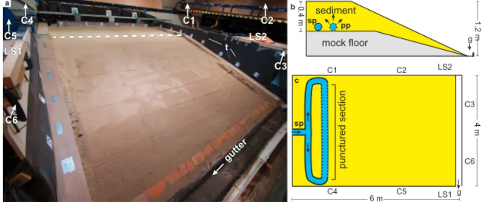
Figure 2. Experimental setup. (a) Oblique photo from downstream end of the flume, showing the initial sediment

surface. Dotted white line indicates the position of the break in slope. Camera locations (C1–C6, above the photographed area) and positions of the laser scanner (LS1, LS2) are indicated. (b) Cross section of the setup, showing the mock floor, subsurface pipe (sp = supply pipe, pp = punctured pipe, and g = gutter). (c) Plan view of the setup, with the same abbreviations as Figures 2a and 2b.

of what to expect in reality. Regardless, these experiments exhibit a range of processes and associated morphologies that could occur in natural landscapes. To bridge the gap between experiment and reality, we analyze the scaling of these processes and evaluate their behavior on natural scales by comparison to a case on Mars.

We modeled the observed processes for a case based on Ravi Vallis (Figure 1b). We chose this outflow channel since its morphology is relatively simple, and the chaotic terrain at the source and the outflow channel suggest it formed in a single event [Leask et al., 2006], in contrast to the more complex collapsed chaotic terrains and multiple incision events observed, for example, at Iani Chaos and Ares Vallis [Warner

et al., 2011, 2009]. We aim to discover processes that result from pressurized groundwater outflow, and

we investigate their capability to generate large floods and assess the associated morphological features. Specifically, we intend to determine what outflow processes are capable of producing the morphologies of the Martian outflow channels, and we are seeking processes that were previously overlooked and thus not present in existing models of Martian paleohydrology. Additionally, our landscape evolution models provide insight into the morphological development of the simulated outflow processes, and these results will therefore be of significant value for interpreting the morphology of the outflow channel source regions.

In a previous set of experiments, Marra et al. [2014] created an overview of landscapes resulting from crater-lake overflow, groundwater sapping, and also pressurized groundwater outbursts. These experiments showed that a complex interaction of processes is responsible for the formation of source areas. However, these experiments were relatively small and did not show morphological details indicative of the individual processes. In this paper, we explore pressurized groundwater in much more detail using a larger-scale experimental setup. Also, in addition to this previous work, we upscale the experimental results to the conditions for Mars using numerical modeling.

2. Experimental Setup

We conducted a series of experiments in the Total Environmental Simulator facility at the University of Hull (details at www.hull.ac.uk/tes) to study the outflow processes and resulting morphology produced by different groundwater pressures applied via different inflow rates at the base of a block of sediment.

All experiments began with the same initial landscape topography constructed from sand overlying a block-work base. We used sand with a median grain size of 0.7 mm, which optimizes permeability for groundwater and transportability by surface runoff [e.g., Marra et al., 2014]. The width of the sediment surface was 4 m with an elevated flat area of 1.7 m which was followed by a 3.5 m long slope with a gradient of 0.22 m/m (Figure 2). The groundwater outflow occurred in the flat area above the slope. The sloping section was designed to ensure the development of surface flows that produced incising channels. The sediment covered a partially sloping impermeable floor to reduce the total amount of sediment required

Table 1. Experiment Runsa

Experiment Duration Q(L/s) V(m3_{) p(kPa) Δp(kPa) TL Interval Video}

1: Low pressure 70 min 0.4 105 4.2 - 30 s Video S1 2: Medium pressure 12 min 0.9 38.4 9.5 3.1 5 s Video S2 3: High pressure 10 min 1.8 46 19.1 11.1 5 s Video S3

a_{Showing duration of the experiments, discharge Q, total volume of waterV, estimated fluid}

pressurep, overpressureΔp, the interval of the time-lapse (TL) images and the corresponding videos in the supporting information.

for model construction. This floor was flat for 2.6 m and the slope was 0.11 m/m for another 2.6 m. An impermeable membrane was used to seal the floor and walls. A rough geotextile fixed to the top of the smooth membrane layer was installed to prevent the possibility of the entire block of sediment from sliding downslope at the contact. The total sediment depth was 0.4 m in the upstream flat section, wedging out toward the downstream end.

We simulated the release of groundwater using a 25 mm diameter pipe, punctured with several hundred 3 mm holes, 0.4 m below the sediment surface (Figures 2b and 2c). The pipe was installed as a ring main with no outflow except through the punctured holes and was fed from the center to ensure an equal pressure distribution. The punctured holes were located in a straight section of the pipe, perpendicular to the surface slope, and this section of pipe was wrapped in a 0.5 mm fabric mesh to prevent clogging by sediment and thus also ensuring uniform groundwater flow from the punctured holes in the flat pipe section.

We performed three experiments using the described setup each with different groundwater inflow rates (Table 1). We estimated the fluid pressure and pressure in excess of the lithostatic pressure (Table 2) at the base of the setup using Darcy’s law (Q = KA dh∕dz), with K = 40 m/d, a depth of 0.4 m and a seepage area of 4 m × 0.2 m = 0.8 m2_{, which is the observed seepage area in the experiments. The pressure is likely to}

have changed during the experiment due to different dynamics of the outflow processes (which also voids the Darcy equation). Nevertheless, these estimates give an idea of the pressure regimes in each of the three experiments with a pressure (1) below, (2) slightly above, and (3) well above the lithostatic pressure (Table 1).

In contrast to the Martian setting, our setup does not feature a capping cryosphere on top of an aquifer, which could cause a buildup of groundwater pressure. Instead, the pressure in the experiments was applied directly from a pump, and we did not study the processes responsible for breaking a confining layer. It was not the purpose of the experiments to study the entire aquifer system since our aim was to study the outflow processes resulting from pressurization and not the processes leading to pressurization. Although the experiments were motivated by the Martian setting, we aimed for generic results that can also be applied to other systems.

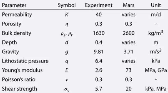
Table 2. Substrate Properties for Experiment and Marsa

Parameter Symbol Experiment Mars Unit Permeability K 40 varies m/d

Porosity 𝜂 0.3 0.3

-Bulk density _𝜌s,_𝜌r 1630 2600 kg/m3

Depth d 0.4 varies m

Gravity g 9.81 3.71 m/s2

Lithostatic pressure q 6.4 varies kPa Young’s modulus E 2.6 73 MPa, GPa Poisson’s ratio _𝜈 0.3 0.3 -Shear strength 𝜎_s 5.7 20 kPa, MPa

a_{Values forE,𝜈, and𝜎}

sare based on Pakpour et al. [2012]

(Experiment) and Schultz [1993] (Mars).

We captured the evolution of the experiments using time-lapse photography from a range of viewing angles. The time-lapse setup consisted of six Canon PowerShot A640 cameras mounted around the experimental setup (see C1–C6 in Figure 2), which were synchronously triggered at set intervals. These intervals differed from 30 s to 5 min, based on the morphodynamic speed of the ongoing experiment (values in Table 1). For detailed morphological analysis and morphometrical analysis, we created digital elevation models of

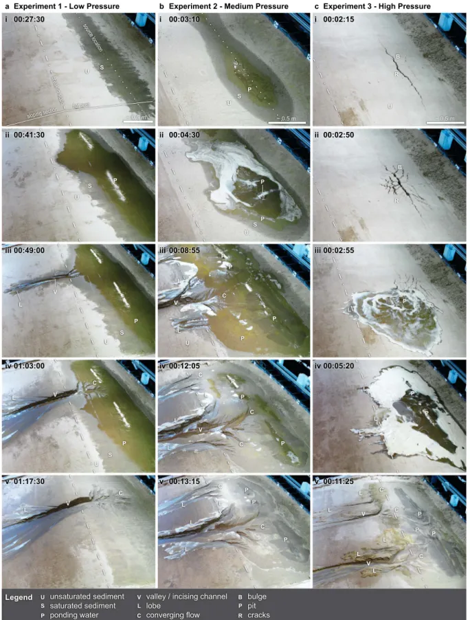
Figure 3. (a–c) Stills from time-lapse video for all three experiments from camera C1 (Figure 2). Dash-dotted line indicates break in slope (see Figure 3a-i), dotted

line shows location of subsurface source (see Figure 3a-i, not repeated in other panels). Light-toned floating material in Figures 3b-ii, Figure 3c-iii, and Figure 3c-iv is foam floating on the water. Approximate scale bars are given in first frames (Figures 3a-i, 3b-i, and 3c-i). Please note perspective distortion and that later images show more of the experiment. For full videos, the reader is directed to the supporting information.

Figure 4. (a–c) Shaded relief with color-coded erosion maps and (e–f ) stitched orthorectified photos of the final

morphology of all three experiments. Figures 4a and 4d are experiment 1, Figures 4b and 4e are experiment 2, and Figures 4c and 4f are experiment 3. The scale shown in Figure 4a and color bar in Figure 4c apply to all panels.

the final surface morphology at the end of each experiment run via point-cloud elevation data obtained using a Leica ScanStation 2 terrestrial laser scanner. Scans were obtained from two opposing directions to eliminate data shadows within the scanned area (see Figure 2). These point-clouds were oriented and placed into the same coordinate system based on fixed targets in the experimental setup using CloudCompare (version 2.4). The combined scans were gridded to 2 mm elevation models using a linear triangulation interpolation algorithm within ArcGIS (version 10.1 SP1).

3. Experimental Results

In this section, we describe the morphological development of the pressurized outflow experiments and link the observed morphology to responsible processes. Please refer to the supporting information for videos of the experiments.

3.1. Experiment 1: Low Pressure

The experiment with the lowest pressure was fed with groundwater for 70 min at a discharge of 0.4 L/s, which corresponds to a pressure well below the lithostatic pressure of the sediment (Table 1). The surface of the sediment remained dry in the first 20 min of the experiment. After 20 min, the surface above the groundwater source became visibly saturated (Figure 3a-i), and the spatial extent of this saturated region

grew radially. From approximately 30 min into the experiment, the seeping groundwater began to pond, forming a radially expanding, shallow lake on the flat part of the initial surface (Figure 3a-ii). After 43 min, this lake reached the top edge of the slope and water started to flow downhill over the sloping surface (Figure 3a-iii).

Seepage continued during the experiment, and the surface reservoir remained present until the water supply ceased at the end of the experiment run. The outflow of groundwater to the surface through artesian seepage in this experiment did not produce visible morphological features on the flat surface although darker, fine sediment was deposited at the outer edges of the surface reservoir.

The overflow from the lake resulted in the formation of a channel (Figure 3a-iv). The channel head consisted of a feather-shaped tributary with multiple radially extending channels due to the convergence of flow from the broad reservoir lake into the relatively narrow channel (Figures 3a-iv/3a-v, 4a, and 4d). Incision of these channels resulted in erosional islands (Figure 5a). The individual channels grew in a headward direction extending further into the reservoir lake. As a result, some of the initial inlet channels were abandoned. Furthermore, remnant grooves at the flanks of the channel show the location of the initial lake outlet (Figure 5a).

As the system evolved, the entire lake drained through a single outlet channel, which was much smaller than the seepage area itself. This is a common occurrence in draining lakes and often generates catastrophic events due to the positive feedback between discharge and erosion [e.g., Cantelli et al., 2004]. The result in this experiment was that this funneling transformed the nonerosive seepage flow into a surface flow with erosive power on the slope. Together with the formation of the channel, sieve lobes developed at the down-stream end of the initial channel (Figures 3a-iii and 3a-iv). These lobes formed in areas where the sediment was still unsaturated, due to infiltration of water from the sediment-rich flow to the unsaturated substrate. As the sediment around the channel became saturated, the deposition of these lobes ceased and the flow incised. As a result, the deposition of these lobes gradually moved downslope. The channel avulsed as lobes grew too large in size.

Incision of the channel resulted in the formation of a valley. Incision began at the overflow location at the break in slope and extended downslope synchronous with lobe formation, resulting in an increased incision rate during the experiment. Incision was strongest in the upstream part of the slope and further downstream the eroded material deposited forming an alluvial fan (Figures 4a and 4d). Due to a

combination of channel incision and lateral erosion, multiple terraces formed, which were narrow but deep upstream and broad but shallow downstream (Figure 4a). The downstream terraces became deeper and narrower as the incision increased in the latter part of the experiment.

Overall, the valley in this experiment formed in one event but the resulting landscape contains a wide range of morphological elements that formed in different stages of the experiment run. The final landscape contains lobate deposits formed in an early stage of the experiment and several abandoned channels and corresponding terraces due to incision of the channel (Figure 5a).

3.2. Experiment 2: Medium Pressure

Experiment 2 had an intermediate pressure just above the lithostatic pressure at a water influx rate of 0.9 L/s for 12 min (Table 1). The first 4 min of experiment 2 developed in a similar sequence to the first 30 min of experiment 1, but at a much faster rate. After 2 min, the area above the inflow pipe became saturated and after 3 min seepage resulted in ponding water at the surface (Figure 3b-i). Beginning at 3.5 min water boils emerged in the source area (Figure 3b-ii). The boils migrated through the source area and persisted until the end of the experiment. We interpret these features as subsurface conduits forced by the excess pressure as the groundwater pressure was higher than the lithostatic pressure. We observed sand exiting the fissures which resulted in a source depression and deposition around these pits (Figures 4b, 4e, and 5b).

Similar to experiment 1, a shallow reservoir lake developed in the source area (Figure 3b-iii). However, due to the erosive nature of the seepage through the conduits, the extent of the reservoir was more clearly delimited in the final morphology than in experiment 1, because there was deposition of sediment from the conduits (Figures 4b and 4e). As overflow from the surface lake drained downslope, sieve lobes similar to those observed in experiment 1 formed due to infiltration of water (Figure 3b-iii). However, in experiment 2 these lobes were deposited closer to the outflow region because the sediment near the outflow zone was still dry when outflow began.

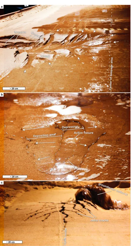
Figure 5. Close-up photo of source areas, photos are taken from close to the sediment surface. (a) Converging flow from

shallow reservoir in experiment 1, arrows indicate flow direction with the arrowheads positioned at developing knick point. (b) Outflow from fissure seepage in experiment 2, showing the outline of an active fissure, depression carved by groundwater outflow, and deposition surrounding this source area, arrows indicate direction of flow. (c) Source area of experiment 3 just after initial outburst showing uplifted deformation with cracks and jet of groundwater emerging from the side of the deformation. This image was taken in between time-lapse frames shown in Figures 3c-ii and 3c-iii.

Subsequent incision progressed in a similar fashion to experiment 1, but due to the heterogeneous and migrating nature of the outflow pattern, the reservoir overflowed at multiple locations resulting in multiple channels of different sizes (Figures 3b-ii, 3b-v, and 4b). Terraces were less clearly visible in this experiment, which was due to the smaller individual channel sizes and shorter duration of this experiment. At the end of the experiment, as the reservoir lake drained, the water level dropped rapidly, so that after sequential abandonment only the largest channels received any flow.

3.3. Experiment 3: High Pressure

The final experiment in the series had a groundwater pressure well above the lithostatic pressure, with a discharge of 1.8 L/s for 10 min (Table 1). At 90 s into the experiment, the sediment surface above the groundwater source pipe began to bulge slightly and cracks formed as a result of the tensional stress related to this bulging (Figure 3c-i). The initial cracks were in the same orientation as the groundwater source pipes and on the top of the bulge. As the bulge grew, the cracks propagated further resulting in a polygonal structure in the bulged area (Figures 3c-ii and 5c). We interpret the bulging of the sediment to result from the formation of a subsurface reservoir, i.e., a lens of water beneath the sediment surface. As the groundwater pressure was far above the lithostatic pressure (Table 1), this excess pressure was able to lift the overlying sediment.

At about 3 min, the subsurface body of water erupted (Figure 3c-iii) and a jet of water about 10 cm in height emerged at the side of the bulged area (Figure 5c). The bulge then subsided within 5 s. At this time, the sediment surface was still dry and unsaturated, so that sieve lobes formed immediately around the source area (Figure 3c-iii). After the initial eruption, outflow continued through small migrating boils of water, similar to those seen in experiment 2 but more erosive (Figure 3c-iv). Pits and surrounding deposits formed at the outflow locations (Figures 3c-v, 4c, and 4f ). During this experiment, foam emerged from the outflow area, which is indicative of a high concentration of fine sediment in the flow, relative to the experiments with lower discharges (Figure 3c-iv).

Overflow from the flat area began after about 5 min. Similar to experiment 2, channels formed at several locations due to the irregular outflow pattern (Figure 4c). Some of the initial channels that overspilled from the flat area at the top of the slope ceased midslope due to infiltration. This effect was more common than in the ther experiments because the lower sediment was not already saturated by the time the overland flow reached it. Up until about 7 min, a few of the channels continued to incise but at a much faster rate than in the previous experiment due to the higher discharges of water. Although the incision rate was fast, the total erosion was less than the other experiments due to the limited duration of this experiment. For the same reason, the formation of terraces was also limited.

4. Scaling of Pressurized Groundwater Outflow Processes

The landscape evolution experiments presented in the previous section show a range of outflow processes which result from different groundwater pressures. In this section, we generalize the experimental results for application to systems at larger scales and in different materials. Based on the processes identified in the experiments, we show the results of a numerical model for a case study at the scale of Ravi Vallis.

A key concept in our analysis is that the landscape in these experiments, although caused by a single driver (applied groundwater pressure), results from multiple but simultaneous active processes that may scale differently from laboratory experiments to natural landscapes. The final landscape consists of several morphological elements resulting from these different processes. Not all processes behave the same across different scales and thus the landscape resulting from real-world systems is likely to be different from a geometrically scaled version of the experiments. To generalize our experimental results, we therefore study the individual processes from the experiment, provide equations for these processes, and evaluate the resulting morphological behavior under different conditions.

We distinguish between the hydrology and hydraulics of outflow and the resulting surface processes. In the experiments, we observed three types of outflow processes (Figure 6): (1) artesian seepage, (2) fissure seepage, and (3) subsurface reservoir eruption. Artesian seepage results from vertical groundwater movement. Fissure seepage occurs when fissures or conduits are formed within the subsurface; these may be physical voids or weaker areas with much higher permeability compared to their surroundings, such that they act as conduits or collapse and become fissures under high pressures. Groundwater eruptions are

Figure 6. Three modes of pressurized outflow of groundwater from a confined aquifer: (a) artesian seepage through

porous media, (b) turbulent flow through fissures, and (c) outflow through fissures after buffering in subsurface reservoir.

the result of surface collapse and expulsion of a subsurface reservoir. In the experiments, the groundwater pressure created the space for such a reservoir, but preexisting voids can be part of this process as well. Within all three experiments, after groundwater outflow had begun, we identified two main processes in the experiment: fluvial incision and the deposition of sedimentary sieve lobes. Below, we will first analyze observations from the experiments regarding the development of a subsurface reservoir as a result of high groundwater pressure. Then, we present a groundwater outflow model and its results based on the observed outflow processes in each of the experiments.

4.1. Subsurface Reservoir Development

In the experiments with the highest groundwater pressure, the surface above the groundwater source bulged and cracked before the groundwater flowed out (Figure 3c-ii), probably due to the expansion of a subsurface body of water as a result of a groundwater pressure that was in excess of the lithostatic pressure. This subsurface reservoir was able to form because the inflow of water at the base of the sediment was higher than the maximum discharge through the sediment and this mechanism is only possible if the pressure from the groundwater is high enough to deform the material above. This process of deformation due to pressure is known as flexure and is similar to laccolith formation in volcanic settings [Turcotte and

Schubert, 2002]. In this section, we discuss the ability of pressurized groundwater to deform the surface and

create space for a subsurface reservoir for both the experiment and in a Martian setting.

4.1.1. Flexure Processes

For a subsurface reservoir to be filled with fluid from deeper sources, fluid pressures in excess of the lithostatic pressure are required. On Mars, the overlying cryosphere would bend as a result of its capacity to support elastic stresses. The sand in our experiments is moist, and capillary forces can also produce macroscopic elastic behavior [Pakpour et al., 2012], resulting in flexural behavior. An approximation of the deformation w as a function of distance from the center of the deformation, x, is (after Turcotte and Schubert [2002], definitions in Figure A1)

w(x) =−Δp

24D (

x2− a2)2 (1)

where Δp is the overpressure at the base of the deformed layer (e.g., sediment layer or cryosphere), a is the radius of the deformation, and D is the flexural rigidity, which is

D≡ ET

3

12(1 −𝜈2₎ (2)

where E is Young’s modulus,𝜈 is Poisson’s ratio (values in Table 2), and T is the thickness of the deformed layer. Flexure is driven by the work of the fluid. The radius a of the uplifted area is given by (see Appendix A4 for derivation)

a≥ 1

2T √

6 ≈ 1.2T (3)

The minimum radius is achieved only when all work by the fluid is converted into elastic strain (flexure). In practical situations a will be larger because part of the work is used to drive permanent deformation of the deformed layer.

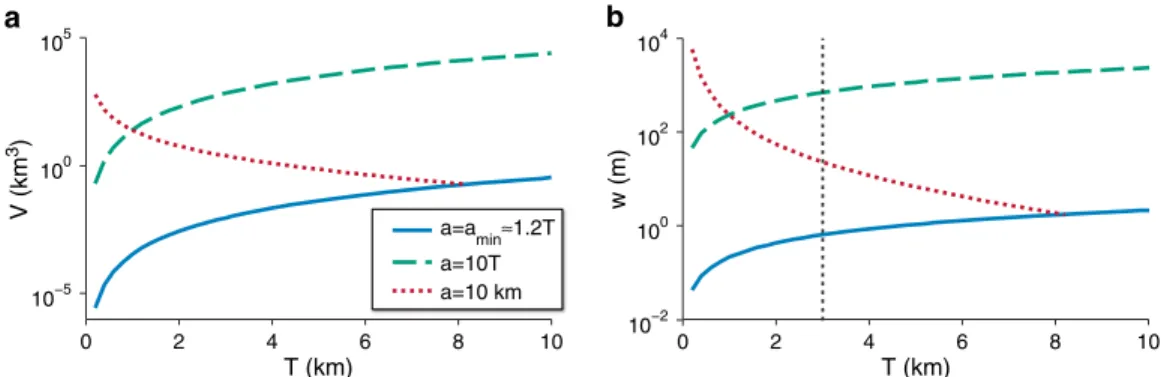
10−5 100 105 104 102 100 10−2 V (km 3) a=a_min≈1.2T a=10T a=10 km 0 w (m) 0 2 4 6 8 10 T (km)

a

b

2 4 6 8 10 T (km)

Figure 7. Flexure deformation and volume. (a) Maximum reservoir volume before collapseVand (b) deformation at the center of the bulgew(0)as a function of cryosphere thicknessTfor the minimum deformation radius required for flexure (a = amin), fora∕T = 10and a constant value ofa = 10km. Vertical dashed lines representT = 3, which is used in

the analysis.

We are interested in the potential volume of a reservoir created by this process. Maximum uplift and reservoir volume are limited by the shear strength𝜎sof the deformed layer. Upon failure of the entire

deformed layer, stored elastic strain energy is dissipated. If we assume that a vertical shear fracture develops, we can calculate the maximum excess pressure by equating the elastic strain energy to the energy due to fault slip (see Appendix A5 for derivation and rationale):

Δp_max=𝜎sa 4 2T4 [ 4 15 (_a T )5 +2 5 (_a T )3]−1 (4)

Therefore, the maximum volume, Vmaxis given by

V_max=𝜋Δp 72Da

6 ₍₅₎

4.1.2. Flexure in Experiments and on Mars

Using the derivation from the previous section, we calculate the flexure for our experimental setting and for Martian cases. For our experimental setting consisting of granular material, the shear strength𝜎sis related

to the normal stress𝜎 following the Mohr-Coulomb criterion:

𝜎s=𝜎 tan(𝜙) + c (6)

For our sediment we assume a value of tan(𝜙) = 0.8 and an added cohesion strength c of 0.6 kPa due to an initial small water content [Mitchell and Soga, 2005; Richefeu et al., 2006]. The initial normal stress is the lithostatic pressure, which was 6.4 kPa at the base of the 0.4 m sediment layer (Table 2), yielding a shear strength of 5.7 kPa. In the experiments we observed a deformed area with a radius of a = 0.7 m (Figure 5c). We assume Young’s Modulus (E) of 2.6 MPa, based on a shear modulus of 1 MPa for similar moist beach sediment [Pakpour et al., 2012]. The deformation w(0) due to flexure by an overpressure of Δp=11.1 kPa (Table 1) is 7.2 mm. In the experiments, we observed a higher deformation of about 3 cm. This difference can be explained by a decrease of the effective thickness of the layer due to the formation of cracks and saturation of the lower part of the sediment. The deformation of 3 cm is achieved with a lower thickness of

T = 0.25 m, with all other parameters being equal.

For the case on Mars, we can estimate the material properties (Table 2), but values for cryosphere thickness and deformation radius are poorly constrained. The minimum radius of the subsurface reservoir required for flexure depends on cryosphere thickness T and for an increasing T and corresponding aminor a higher

ratio of a∕T, the amount of flexure and corresponding reservoir volume increases (Figure 7). For fixed val-ues of a, the deformation and volume decreases with higher valval-ues of T as this provides more resistance to deformation.

As an exemplary case, we take the source area of Ravi Vallis as an example. We consider a cryosphere thick-ness of 3 km and a deformation radius a of 50 km, which is similar in size as the area with fractures just upstream of Ravi Vallis. This results in a required excess pressure for breaking the cryosphere Δp = 2.2 MPa,

and a subsurface reservoir volume of 8500 km3_{. After failure, this volume is ejected to the surface,}

generat-ing a high discharge peak. This initial outburst is close to the estimated volume required to form Ravi Vallis in an single flood, which ranges from 11,000 to 65,000 km3_{[Leask et al., 2006]. In the next section, we model}

the effect of this subsurface reservoir on the outflow hydrograph, together with other possible outflow processes.

4.2. Outflow Processes

In the experiments, we observed three groundwater outflow mechanisms which each had a different efficiency in terms of the rate at which water was output from the subsurface. To quantify the relative effi-ciencies of these processes at a real-world scale, we model them numerically in a confined aquifer setting. Here we present equations to model the three different groundwater outflow processes, and, based on these equations, we show a suite of model results for Ravi Vallis under different outflow conditions. These results are given as an exemplar to illustrate the potential behavior of the observed experimental processes at a planetary scale.

4.2.1. Groundwater Flow and Artesian Seepage

The hydraulic head development in a pressurized aquifer is given by the groundwater flow equation, which is the divergence of groundwater fluxes:

Ssdh

dt = −∇⋅ (−K∇h) (7) where K is the hydraulic conductivity of the material (m/s), h is the hydraulic head, and Ss is the specific storage (1/m), which quantifies the ability of an aquifer to discharge groundwater:

Ss =𝜌g(n𝛽water+𝛽aquifer) (8)

where𝜌 is the density of water, n is the porosity, 𝛽wateris the compressibility of water (4.4 × 10−10Pa−1), and

𝛽aquiferis the compressibility of the aquifer, which is a function of depth and effective stress state [Hanna and

Phillips, 2005].

Seepage from normal, Darcian, groundwater flow (Figure 6a) is calculated as

Qseep= −KiA (9)

where Qseepis the total seepage discharge (m3/s), i is the hydraulic gradient (m/m, i = h∕d, h is the head

difference which equals the hydraulic head at the top of the confined aquifer and d is the distance to the surface which is here the thickness of the cryosphere T), and A is the seepage area (m2_).

4.2.2. Fissure Outflow

In the medium and high-pressure experiments, water reached the surface through fissures (Figure 6b). Water boils in the outflow area show the relatively high outflow discharge of this process compared to seepage. Assuming turbulent flow through fissures, the discharge is given by [after Andrews-Hanna

and Phillips, 2007; Head et al., 2003] (note that his equation is the flux in m3_{/s, where equation (5) in}

Andrews-Hanna et al. [2007] is in m/s) Qfiss= √ gwfiss fw i⋅ wfiss⋅ Nfiss⋅ A (10)

where Q_fissis the total outflow through the fissures, w_fissis the width of the fissures (m), f_wis a Darcy-Weisbach friction factor (dimensionless), and Nfissis the spatial density of fissures (number/m).

4.2.3. Subsurface Reservoir Eruption

In the high-pressure experiment, groundwater collected in a subsurface reservoir before it outflowed onto the surface. This reservoir system acts as a buffer, prior to a sudden discharge occurring at the surface (Figure 6c). Although the outflow is governed by the same equation as above (equation (10)), the development of hydraulic head at the base of the fissures, and thus, the discharge from the fissures differs. When an aquifer is the water source for a fissure, the permeability limits the drawdown of water from that aquifer. In a subsurface reservoir created by flexure, the pressure in the reservoir is always at least equal to the lithostatic pressure. Here we assume a linear decrease in pressure with decreasing reservoir volume. As outflow begins the pressure is equal to that of the source aquifer and decreases to lithostatic pressure when empty.

Figure 8. (a) Schematic hydrological model setup and (b) a visual representation of groundwater flow, whereRis the radial distance from the center of the outflow andzis the depth.

4.2.4. Groundwater Outflow Models

We studied the efficiency and behavior of the outflow system described above in a numerical model. This numerical model has a similar setup to the model by Andrews-Hanna and Phillips [2007]. We modeled a pressurized aquifer beneath a confining cryosphere of thickness d, with an aquifer thickness of 20 km (Figure 8a). The aquifer was cylindrical with an outflow region in the center of radius Routflow, the total

extent of the aquifer was 2 times Routflow, which was sufficiently large that no groundwater drawdown

occurred at the outer boundary of the model within one outflow event (Figure 8b). This aquifer had an initial overpressure Δp and was not recharged at any boundary node. We used the hydrological values provided by Hanna and Phillips [2005]. For simplicity, and since we are interested in an order-of-magnitude estimates to show the main differences in processes, we ignore the poroelasticity and used the static values for megaregolith for𝛽aquiferwhich is a function of depth.

We modeled the groundwater outflow in MATLAB using the equations described above (parameters given in Table 3) and an implicit finite difference numerical scheme. We schematized the described setting in an axisymmetrical grid with grid cells of 1 km long in horizontal and 100 m in vertical direction. Fluxes between cells were calculated at cell edges and hydraulic pressure was calculated at cell centers. The model was numerically stable and ran with a time step of 500 s.

We modeled groundwater outflow in a region with the dimensions of Ravi Vallis, with an outflow radius of 20 km and a confining cryosphere depth of 3 km, which falls within the range of estimates discussed in Lasue et al. [2013]. The initial overpressure of the entire aquifer was set to 0.5 MPa unless noted other-wise. In the outflow region, the three different outflow modes described above were used. For the seepage case, the outflow was effectively an extension of the aquifer model. For the fissure outflow case, the model balanced the outflow flux to the surface with the aquifer able to supply this flux. In case of a subsurface reservoir, the model started with an initial reservoir volume of 8500 km3_{, which is based on the flexure}

volume estimate of Ravi Vallis described in the previous section. This reservoir starts with the same pressure

Table 3. Outflow Model Parameters

Parameter Symbol Value(s) Unit Outflow radius R_outflow 20 km

Depth d 3 km

Permeability aquifer k(atz = −d) 10−14_{, 10}−12 _m2

Permeability upper layer k_seepage 10−13_{, 10}−12 _m2

Overpressure Δp 0.5, 5 MPa

Reservoir volume V_reservoir 30,000 km3

Darcy-Weisbach friction loss f_w 0.025 -Fissure width w_fiss 0.025, 0.5 m Fissure density N_fiss 1/1000, 1/500 m−1

as the aquifer and decreases linearly to lithostatic pressure as the reservoir depletes. The groundwater flux from the aquifer recharges the reservoir and fissure flow to the surface comes from this reservoir. When the reservoir is empty, the model continues as a fis-sure outflow model with outflow to the surface from the groundwater directly. There are a number of key differences discernable in the hydrographs produced by the different outflow mechanisms and model parameters (Figure 9). For the artesian seepage outflow models, a higher initial

Time (days) Discharge (m 3/s) 0 10 20 30 40 50 102 103 104 105 106 107

Q_max Ravi Vallis Artesian seepage ... with high ΔP ... with high k Fissure outflow ... with high wfiss

... with high k

Subsurface reservoir outflow ... with larger w_fiss

... with higher N_fiss

Figure 9. Hydrographs for different outflow models. Red lines are outflow models with artesian outflow at the source

area, blue lines are the result of fissure outflow models, and green lines are the subsurface reservoir outflow model results. Solid lines are the base models (lowΔp, lowk, lowW_fiss, and lowN_fiss; see Table 3 for values). Dashed red line shows run with increased aquifer pressure. Dotted lines represent model runs with high-permeability values for the arte-sian seepage and fissure outflow cases. Model runs with increased fissure size (dashed blue line) is not visible as it plots on top of the baseline run. For the subsurface reservoir outflow model, the dashed line represents run with larger fis-sures (higherw_fiss) and the dotted line with both larger and more (higherN_fiss) fissures. Shaded red area is the range of maximum discharge estimates for Ravi Vallis of Leask et al. [2006] (10–30×106_m3_{/s), based on fluvial morphology.}

overpressure of 5 MPa (Figure 9, dashed red line) only produces slightly higher discharges than the 0.5 MPa baseline model (Figure 9, solid red line). The main parameter that produces a significant increase in discharge is the permeability, a tenfold increase results in a similar increase in the magnitude of discharge (Figure 9, dotted red line). The fissure outflow models produce higher discharges than the seepage model for the same aquifer properties (Figure 9, solid and dotted blue lines). An increase in size and number of fissures does not result in higher outflow discharges, since the outflow is limited by the ability of the aquifer to supply groundwater to the fissures (the dashed blue line overlies the baseline run in Figure 9).

The hydrographs from subsurface reservoir eruptions are substantially different from the seepage and fissure outflow hydrographs. The baseline model with the same fissure properties as the fissure outflow models has the same initial discharge because the underlying pressure is equal to that of the fissure models. However, the discharge from the reservoir hardly decreases as the pressure in the reservoir is at least the lithostatic pressure during the drainage of the reservoir (Figure 9, solid green line). For such small fissures, the reservoir does not deplete in the 60 days shown in Figure 9. However, for the collapse of a subsurface reservoir we expect much larger fissures. An increase in fissure size (w_fiss= 0.5 m) and number of fissures (Nfiss= 1/500 m−1), yields a high discharge peak, which is followed by an outflow that is similar to outflow

from groundwater when the reservoir is depleted (Figure 9, dashed and dotted green lines). The estimates of the discharge peaks in Ravi Vallis (107_m3_{/s) are of the same order of magnitude as the peak discharge}

produced by these subsurface reservoir outbursts (Figure 9).

5. Discussion

In this paper, we present a set of landscape evolution experiments wherein we simulate the outflow of groundwater. These experiments were motivated by the hypothesized pressurized groundwater source of the outflow channels on Mars. We assume a megaregolith aquifer [Hanna and Phillips, 2005], with the presence of a confining cryosphere [Clifford and Parker, 2001] on top of this aquifer likely to have contributed to the pressurization of the aquifer. The experiments showed that different outflow processes are driven by the underlying groundwater pressure. We observed three different types of groundwater outflow, with an increasing order of driving pressure: (1) artesian seepage, (2) outflow through fissures, and (3) the eruption from a subsurface reservoir. We presented an analysis of the potential flexure of a cryosphere due to

superlithostatic groundwater pressure and showed that this mechanism is capable of producing a subsurface reservoir.

Here we first discuss the general outflow channel morphology and the efficiency of these outflow processes, before addressing the relationships between Martian chaotic terrains and their outflow channels.

5.1. Outflow Channel Fluvial Morphology

The outflow processes from the groundwater source in our experiments contrasted between different groundwater pressures, but the fluvial processes downstream were similar and resulted in similar morphologies in all three experiments. The channel morphology can be split into four zones. (1) Proximal to the source, flow convergence formed a broad source to a narrow channel giving rise to the incision of feather-shaped tributaries. In places this zone has islands that are erosional remnants. (2) Immediately downstream of this area where the flow converged into one channel, the incision was strongest resulting in a narrow and deep channel with terraces. Adjacent to the valley, we observed groove marks which indicate that the channel was initially wider. (3) Further downstream, the initial outflow resulted in the deposition of sedimentary lobes due to the infiltration of water into the still unsaturated substrate downstream. These lobes were partially eroded by the subsequent incision. The final channel and adjacent terraces here are broader and shallower than upstream. (4) In the distal part, the channel deposited the material eroded upstream which resulted in an alluvial fan.

The last three zones of the experimental morphology described above are consistent with the Sandur facies of glacial outburst floods which are often considered as an analog for the Martian outflow channels [Rice

and Edgett, 1997]. Since the entire range of features from upstream to downstream and from incision to

deposition are present, we are confident that all main morphological features are present and consistent in our experiments. The formation of outflow channels in reality may have been characterized by other processes, for example, by density currents [Ivanov and Head, 2001], but the general transition in morphology observed here is similar.

The converging shape of the source area is also typical for outflow channels [e.g., Komatsu and Baker, 1997], but is emphasized in our experiment due to the transition from a completely flat source area to a steep sloping area. This setting is more similar to the catastrophic outflow from crater lakes, which also feature such typical outlet fans [Marra et al., 2014].

In our experiment, no teardrop-shaped islands formed in the channels. Such islands are often located downstream of obstacles in outflow channels and are likely to be the result of differential resistance to erosion in material that is more heterogeneous than the experimental sediments. Islands observed in our source area are the result of rapid incision and are preserved due to limited lateral movement of the tributary channels.

5.2. Seepage and Fissure Outflow

In the low- and medium-pressure experiments, groundwater reached the surface by seepage and fissure flow, respectively. In the case of seepage, groundwater slowly wetted the surface after which seepage began. This process did not result in the development of any erosive morphology directly; lake deposits and the incised channels further downstream are the only evidence for groundwater outflow. Artesian seepage occurs at surface depressions and is only possible when the aquifer is unconfined at the location of outflow. Such a system requires either the absence of a confining layer in combination with a local source of pressurization, e.g., tectonics or an impact, or a discontinuous confining layer.

In the experiment with fissure flow, the groundwater pressure itself resulted in the formation of fissures, which is likely to have occurred after the sediment became saturated and thereby lost its cohesive strength. At the planetary scale, in systems with a rock or a cryospheric surface, such fissures may emerge from tectonic activity, magmatism (e.g., dike intrusion), meteor impacts, or from hydrofractures (similar to the experiments with high groundwater pressure). Due to the existence of fissures in the experiment, water reached the surface at only a few locations. In the resulting morphology, these outflow locations were visible as sand volcanoes, consisting of pits surrounded by lobes of sediment. Such outflow through fissures on Mars requires a confined pressurized aquifer; the outflow locations are the result of the fissure locations and are unrelated to the local topography.

Our numerical modeling results show that seepage and fissure outflow processes are similar in efficiency because groundwater flow limits the supply of groundwater to the outflow area. The maximum discharge is

primarily a function of the hydrological properties of the aquifer that supplies the groundwater. Our model results for Ravi Vallis show that these processes are capable of producing a discharge peak that ranges from 103_{to 10}5_m3_{/s, depending on aquifer properties. However, morphological evidence implies a much higher}

discharge peak of 107_m3_{/s [Leask et al., 2006].}

Previous model studies provide similar magnitudes as our model results. For example, a discharge of 8 × 106_m3_{/s was estimated for Iani Chaos [Andrews-Hanna and Phillips, 2007], which has a 100 times}

larger outflow area than our model. Our optimistic aquifer properties are similar to the properties used by

Andrews-Hanna and Phillips [2007], which is a very permeable hydrofractured aquifer. The model of Manga

[2004] produces discharges of 0.5 to 2.5 × 106_m3_{/s for Athabasca Valles (Figure 1d), which corresponds}

with peak-discharge estimates of 1–2 × 106_m3_{/s based on bankfull discharge [Burr et al., 2002]. Improved}

methods for discharge estimates based on hydrodynamic models using high-resolution elevation models provide discharges of the same order of magnitude [McIntyre et al., 2012]. In his model, Manga [2004] simulates one large fissure that reaches to the base of a 3 km deep aquifer; in contrast within our model, the fissures are only present in the confining cryosphere on top the aquifer. In addition, Manga [2004] uses a high permeability of 109_m2_{, which may overestimate the groundwater discharge.}

The origin of the fractures that deliver the groundwater to the surface is important. When these fractures are the result of hydrofracturing by the pressurized groundwater itself, the aperture is in the order of millimeters [Andrews-Hanna and Phillips, 2007]. Our model results show that larger fissures do not produce a higher outflow when the groundwater flow from the aquifer is limiting the outflow. However, when considering tectonic fissures that reach deep into the aquifer, as is the case in the Manga [2004] model, the aquifer can supply more water due to the larger contact surface between the aquifer and fissure.

A deep-fissure mechanism seems unlikely for large chaotic terrains, as the drawdown of hydraulic head at a fracture would impede groundwater flow to the downstream areas. Outflow would in this case originate from one deep fracture like the outflow from Cerberus Fossae (Figure 1d) and not from a network of fractures like Iani Chaos (Figure 1c). We thus interpret the fractures in chaotic terrains not to be deeper than the confining cryosphere. Deep aquifers may have fed outflow channels that have a single pit or fissure source. Examples of such source areas are found at Allegheny, Elaver, Walla Walla, Athabasca, and Mangala Valles [Head et al., 2003; Hanna and Phillips, 2006; Coleman et al., 2007b; Komatsu et al., 2009]. In the latter case, the stress that created the fissure may also be responsible for the pressurization of the aquifer [Hanna and Phillips, 2006].

Groundwater outflow by seepage or fissures is, in most cases, limited by the properties of the aquifer that supplies the groundwater. Only models with an optimal setting of fissures protruding deep into the aquifer and unrealistically high aquifer permeability result in outflow discharges that correspond with observed morphological constraints. In the following sections, we discuss mechanisms that could make a limited groundwater outflow flux larger by buffering and funneling surface or subsurface reservoirs.

5.3. Surface Ponding

In our experiments, the collection of groundwater in a surface lake resulted in a discharge peak that exceeds the groundwater flux. In our lowest-pressure experiment (Experiment 1), the final morphology does not show any evidence of the groundwater outflow itself as the seepage flux was too low to produce any morphology. In this case, the erosive power is the result of the surface lake that acts as a buffer and funnel for the groundwater as the total source area for groundwater seepage was larger than the outflow channel width.

Several Martian outflow channels originate from surface depressions, e.g., Ma’adim, Landon, Morava, Elawer, and Okavango Valles [Coleman, 2013; Irwin et al., 2002; Mangold and Howard, 2013]. Similar to our experiments, a groundwater source for these lakes might not be visible in the morphology. Candidates for such systems are depressions with a channel at the outlet but without any inlet channel. The recharge of such lakes by regional artesian seepage suggests the absence of or a discontinuous cryosphere (Figure 6a). Such channels may either be formed before the presence of an extensive cryosphere or the result of gentle cryosphere disruptions due to a slightly pressurized aquifer or regional melting of the cryosphere instead of rupture.

Formation of Ma’adim Vallis is likely the result of release of water from a large lake. The extensive basin collected large amounts of water, possibly from groundwater [Irwin et al., 2002]. Similar to our experiments,

collection of groundwater in a lake is required to achieve a sufficiently large reservoir of water to carve the outflow channel. The low elevation of the Ma’adim source area favors recharge from groundwater and a possible direct path for groundwater recharge is basal melt from the south polar ice cap [Clifford, 1987]. A possible source of water for several basins in Ismenius Lacus that fed Okavango Valles is also recharge by groundwater [Mangold and Howard, 2013]. The individual basins are local depressions, but the entire area has a higher elevation than the adjacent northern plains. Recharge in local depressions suggests the absence of a confining layer, but the recharge in a regionally elevated area cannot be explained without a confined aquifer. The Ismenius Lacus region is therefore a good candidate for a regionally disrupted or partially developed cryosphere.

Former surface lakes also possibly existed in Capri Chasma [Coleman et al., 2007a] or within Valles Marineris [Harrison and Chapman, 2008]. Harrison and Grimm [2008] and Fueten et al. [2014] propose the existence of such lakes in several chaotic terrains and Juventae Chasma to unify the large number of required groundwater outflow events predicted by numerical modeling and the low number of events visible in the downstream fluvial morphology. For such hypothesized lakes that fall entirely within a Chaos or Chasma, the surface depression had to be present pre-chaos formation, or only later outflow events could have ponded [Harrison and Grimm, 2008].

The depth of the highest point of the outflow channel limits the maximum volume of water drained from such a surface lake. The maximum cumulative discharge is attained when the source depression is filled completely, and the channel incises during a single event. For Ravi Vallis, our model case study, the source depression has a surface area of 2500 km2_{, the maximum depth is 3 km, but the depth at the outflow point}

is about 1 km (Figure 1b). Thus, one lake overflow event for Ravi Vallis is limited to about 2500 km3_{of water,}

which is about one fourth of the minimum estimate of 11,000 km3_{required to form this outflow channel}

[Leask et al., 2006], but that estimate requires a very high sediment concentration. Similarly, the estimated maximum volume for a possible lake in Valles Marineris is 110,000 km3_{, about one third of the cumulative}

discharge estimate for Simud Valles based on high sediment concentrations [Harrison and Grimm, 2008;

Harrison and Chapman, 2008]. The discharge from surface lakes is in the right order of magnitude for the

formation of the outflow channels, but only when assuming very high sediment concentrations.

5.4. Subsurface Reservoirs Eruptions

In our high-pressure experiment (Experiment 3), flexure of the surface generated the space for a subsurface reservoir that resulted in high-discharge outflow. Subsurface reservoirs exist in terrestrial settings, for example, beneath the Antarctic ice cap [Dowdeswell and Siegert, 1999] and may have existed on Mars [Rodr´ıguez et al., 2003, 2011]. We showed that flexure by pressurized groundwater is a feasible mechanism in a Martian setting to produce subsurface reservoirs. Below, we discuss this analysis, the outflow efficiency of such a reservoir eruption, and the morphological elements that may indicate its former presence.

For our analysis of flexure in a Martian setting, we assumed the base of a cryosphere as a horizontal layer where pressurized water induces the deformation of the cryosphere at the top. Important factors that determine the amount of flexure, and thus the size of the resulting subsurface reservoir, are the spatial extent of the reservoir and the thickness and strength of the cryosphere.

For our model we used a strength of 20 MPa, based on the strength of basalt [Schultz, 1993]. The strength of the cryosphere may vary depending on the assumed composition. The upper part of the cryosphere is likely to consist of impact ejecta, cemented by pore ice. While at greater depth, the cryosphere is more likely to consist of compacted regolith or basalt. For the uppermost part of the cryosphere, we assume a tensile strength of ice-sediment mixtures, which is about an order of magnitude lower than rock [Lange and Ahrens, 1983]. However, the collapse of the entire cryosphere depends on the emergence of cracks at the base. At depth, the cryosphere consists of rock or fractured rock [Hanna and Phillips, 2005], filled with ice. The strength here is comparable to rock or even higher due to the added strength of ice in the pores. Our modeled cryosphere thickness of 3 km in our example of Ravi Vallis falls well within the estimated range of cryosphere thickness [Lasue et al., 2013]. The thickness of the cryosphere depends on the thermal properties of the lithosphere, geothermal, and solar heat fluxes. The estimated thickness increases with higher latitudes, higher freezing points, and lower lithospheric heat flow [Clifford and Parker, 2001; Lasue

Hesperian and Amazonian. In our subsurface reservoir model, a thicker cryosphere results in higher reservoir volumes; thus, estimates are likely conservative.

The lateral extent of the subsurface reservoir has a large influence on its volume. However, this parameter is poorly constrained since we lack sufficient information on the deep subsurface of Mars. We estimated a minimum size, but subsurface properties have a great influence on where the formation of such a reservoir will start and how large it can become. In our case study, we used a practical approach as we based our deformation radius on the size of the fractured area upstream of Ravi Vallis, which would be the result of the deformation.

Our experiments and model demonstrated that the collapse of a subsurface reservoir is capable of delivering a high discharge peak. Such peak discharges remain high, even when the reservoir volume is small, and may account for a large amount of total erosion in Martian outflow channel systems. In contrast to direct outflow from an aquifer, our model results show that the release from a subsurface reservoir is capable of generating large flood discharges, similar to the estimated discharge peak of 1–3 × 107_m3_{/s that}

is estimated to have formed Ravi Vallis [Leask et al., 2006]. Groundwater outflow continues even after the depletion of the reservoir, but at a lower discharge due to drawdown and reduced groundwater pressure. However, after such a violent initial eruption, fractures in the cryosphere and possibly in the aquifer itself are efficient pathways for the continuation of outflow which acts as a funnel as the affected reservoir region can be much larger than the actual outflow area (Figure 6c). This funneling mechanism can explain the larger volume of water required for an outflow channel compared to the volume created by flexure plus additional subsidence volume.

The morphological evidence that supports the existence of the formation and outburst of a subsurface reservoir are both concentric and radial fractures. The stress pattern in the cryosphere due to flexure predicts the formation of extensional faults at the surface in the center of the deformed area. This was shown in our experiment by polygonal cracks that emerged during the formation of a subsurface reservoir (Figure 5c). Based on our model predictions and our experimental observations, we expect the initial collapse and outflow at the outer limit of deformation. After collapse, the subsurface reservoir drains, resulting in quick deflation. The resulting morphology does not feature the bulge that was present before the outburst. However, there might be cases where such bulge is still present, but there would be no associated outflow channel. In our experiments no new fractures formed during collapse of the reservoir, but in real-world cases we expect the formation of concentric fractures, analogue to the observations from ice-sheet collapse associated with Jökulhlaup events [Björnsson, 2009]. The expected fracture pattern is not only located around the outflow but in the entire area above the subsurface lake.

5.5. Groundwater Outflow Through Chaotic Terrains

Chaotic terrains on Mars have a similar fracture pattern to that observed above the doming reservoir in our experiment. These terrains mainly comprise of polygonal networks of fractures on the chaos floor and concentric fractures around the chaotic terrain [Roda et al., 2014]. In our experiments, the polygonal fractures were the result of surface inflation, while similar patterns have been attributed to subsidence, for example, in Iani Chaos [Warner et al., 2011], Aureum Chaos [Rodr´ıguez et al., 2005], and Aromatum Chaos. These areas also show collapse features beyond the chaotic terrain itself. This indicates that the subsidence extended further than the outflow area itself, which was also the case in our experiments.

Besides Mars, Michaut and Manga [2014] propose a similar mechanism for the formation of chaotic terrains on the Jovian moon Europa, essentially as a result of by liquid water sills in the moon’s ice shell. This mechanism is equivalent to the subsurface reservoirs that formed in our experiment, and the mechanism explains the chaotic morphology without the outflow of water to the surface.

In our flexure model, the amount of subsidence is the result of the preceding bulging. This explains the surface lowering back to its original level but not the formation of chaotic terrains that appear to have collapsed lower than their original level. Disruption of the underlying aquifer and expulsion of subsurface material can explain excess collapse. However, many chaotic terrains show collapse of a kilometer or more which could be explained by collapse into a preexisting cavities like impact basins. Roda et al. [2014] proposed the collapse of buried frozen lakes for chaotic terrains, which explains large amounts of collapse due to the preexisting basin. Indeed, such subice lakes are potential candidates for pressurization.