Evaluation of model-simulated source contributions to tropospheric ozone with aircraft observations in the factor-projected space

(1)

HAL Id: hal-00303158

https://hal.archives-ouvertes.fr/hal-00303158

Submitted on 2 Nov 2007

HAL is a multi-disciplinary open access

archive for the deposit and dissemination of sci-entific research documents, whether they are pub-lished or not. The documents may come from teaching and research institutions in France or abroad, or from public or private research centers.

L’archive ouverte pluridisciplinaire HAL, est destinée au dépôt et à la diffusion de documents scientifiques de niveau recherche, publiés ou non, émanant des établissements d’enseignement et de recherche français ou étrangers, des laboratoires publics ou privés.

Evaluation of model-simulated source contributions to

tropospheric ozone with aircraft observations in the

factor-projected space

C. Shim, Y. Wang, Y. Yoshida

To cite this version:

C. Shim, Y. Wang, Y. Yoshida. Evaluation of model-simulated source contributions to tropospheric ozone with aircraft observations in the factor-projected space. Atmospheric Chemistry and Physics Discussions, European Geosciences Union, 2007, 7 (6), pp.15495-15532. �hal-00303158�

(2)

ACPD

7, 15495–15532, 2007 Evaluation of simulated contributions to tropospheric O₃ C. Shim et al. Title Page Abstract Introduction Conclusions References Tables Figures ◭ ◮ ◭ ◮ Back Close

Full Screen / Esc

Printer-friendly Version Interactive Discussion

Atmos. Chem. Phys. Discuss., 7, 15495–15532, 2007 www.atmos-chem-phys-discuss.net/7/15495/2007/ © Author(s) 2007. This work is licensed

under a Creative Commons License.

Atmospheric Chemistry and Physics Discussions

Evaluation of model-simulated source

contributions to tropospheric ozone with

aircraft observations in the

factor-projected space

C. Shim1,*, Y. Wang1, and Y. Yoshida2,3

1

Department of Earth and Atmospheric Sciences, Georgia Institute of Technology, 311 Ferst Drive, Atlanta, GA 30332, USA

2

Goddard Earth Science and Technology Center, University of Maryland, Baltimore County, Baltimore, MD 21228, USA

3

The Atmospheric Chemistry and Dynamics Branch, NASA Goddard Space Flight Center, Greenbelt, MD 20771, USA

*

now at: Jet Propulsion Laboratory, California Institute of Technology, 4800 Oak Grove Drive Pasadena, CA 91109, USA

Received: 4 October 2007 – Accepted: 18 October 2007 – Published: 2 November 2007 Correspondence to: C. Shim ([email protected])

(3)

ACPD

Full Screen / Esc

Abstract

Trace gas measurements of TOPSE and TRACE-P experiments and corresponding global GEOS-CHEM model simulations are analyzed with the Positive Matrix Factor-ization (PMF) method for model evaluation purposes. Specially, we evaluate the model simulated contributions to O3 variability from stratospheric transport, intercontinental

5

transport, and production from urban/industry and biomass burning/biogenic sources. We select a suite of relatively long-lived tracers, including 7 chemicals (O₃, NO_y, PAN, CO, C3H8, CH3Cl, and

7

Be) and 1 dynamic tracer (potential temperature). The largest discrepancy is found in the stratospheric contribution to 7Be. The model underesti-mates this contribution by a factor of 2–3, corresponding well to a reduction of 7Be

10

source by the same magnitude in the default setup of the standard GEOS-CHEM model. In contrast, we find that the simulated O3 contributions from stratospheric

transport are in reasonable agreement with those derived from the measurements. However, the springtime increasing trend over North America derived from the mea-surements are largely underestimated in the model, indicating that the magnitude of

15

simulated stratospheric O₃source is reasonable but the temporal distribution needs im-provement. The simulated O3 contributions from long-range transport and production

from urban/industry and biomass burning/biogenic emissions are also in reasonable agreement with those derived from the measurements, although significant discrepan-cies are found for some regions.

20

1 Introduction

Tropospheric O₃ has important environmental consequences. Photolysis of O₃ and the subsequent reaction of O(1D) with water vapor (H2O) in troposphere produces the

hydroxyl radical (OH), which is the most important oxidant in troposphere. This tro-pospheric oxidation by OH determines the lifetime of major greenhouse gases such

25

as methane (CH4). The sources of tropospheric O3 include photochemical

(4)

ACPD

Full Screen / Esc

tion within the troposphere and transport from the stratosphere. Many studies have investigated the main sources to tropospheric O₃. Springtime O₃increase is attributed to photochemical production (e.g., Penkett and Brice, 1986 and Liu et al., 1987). A number of studies using 3-D chemical transport models have focused on the effect of intercontinental transport on tropospheric O₃concentrations from Asia to North

Amer-5

ica (e.g., Berntsen et al., 1999; Jaffe et al., 1999; Jacob et al., 1999; Bey et al., 2001). The effect of trans-Pacific transport is particularly noticeable in the spring (e.g., Jacob et al., 1999; Mauzerall et al., 2000; Wild and Akimoto, 2001; Tanimoto et al., 2002; Wang et al., 1998, 2006). On the other hand, the studies based on the observed corre-lations between O3and

7

Be attributed this trend to transport of stratospheric O3(e.g.,

10

Oltmans and Levy, 1992; Dibb et al., 1994).

The observed relationships between tropospheric O3and CO provide additional

di-agnosis of O3 sources (e.g., Fishman and Seiler, 1983; Chameides et al., 1987;

Par-rish et al., 1993). Furthermore, those relationships between simulated CO and O₃offer a reasonable way to evaluate model simulations of O3(e.g., Chin et al., 1994). Later

15

studies using the positive matrix factorization (PMF) method, an advanced multi-variant factor analysis, enabled better quantifications of source contributions to tropospheric O3 and diverse volatile organic compounds (Wang et al., 2003b; Shim et al., 2007).

PMF analysis of the measurements obtained during the Tropospheric Ozone Produc-tion about the Spring Equinox (TOPSE) experiment found that the increasing seasonal

20

trend of springtime O3 at northern mid and high latitudes is attributed more to

tropo-spheric O3production and transport, even though O3 transport from the stratosphere

is the largest contributor to O₃variability (Wang et al., 2003b).

One drawback noted in the study by Wang et al. (2003b) is that the PMF results can-not be directly compared to 3-D model results. In this work, we apply the PMF method

25

to the simulation results of a global 3-D chemical transport model (GEOS-Chem). As such, we can compare the PMF results to model simulations and evaluate the perfor-mance of GEOS-Chem on the basis of aircraft measurements. A main issue is how model simulated factor contributions to O₃ variability compare with those based on

(5)

ACPD

Full Screen / Esc

the measurements. Unlike direct comparisons between observed and simulated trace gases, measurements and corresponding model results are first projected with PMF onto the factor space before model evaluation. In the factor space, a suite of chemi-cals can be evaluated simultaneously in a consistent and objective manner, which is difficult to achieve using direct comparisons between the measurements and model

re-5

sults. Aircraft measurements from two aircraft field campaigns, TOPSE and TRAnsport of Chemical Evolution over the Pacific (TRACE-P, March–April 2001) experiments are used. We describe data selections from TOPSE and TRACE-P and GEOS-CHEM sim-ulations in Sect. 2.1. The PMF method is explained in Sect. 2.2. Evaluation of model results in the projected factor space is discussed in Sect. 3. Conclusions are given in

10

Sect. 4.

2 Methodology

2.1 Measurements and GEOS-Chem simulations

Figure 1 shows the measurement regions during TOPSE and TRACE-P. The TOPSE experiment (February–May 2000) was conducted to investigate the photochemical

15

transition during spring at northern mid and high latitudes (Atlas et al., 2003). The TRACE-P experiment (March–April 2001) was conducted to investigate the Asian out-flow to the Pacific (Jacob et al., 2003). Both experiments took place during spring when significant transport of O₃from the stratosphere is expected (e.g., Wang et al., 1998b and references therein)

20

In this study, we analyze relatively long-lived chemical tracers including O3, total

re-active nitrogen (NO_y), peroxyacetylnitrate (PAN), CO, C₃H₈, CH₃Cl, and Beryllium-7 (7Be) and one dynamic tracer (potential temperature). Those tracers other than O3

generally have specific primary source characteristics. NOy is a good tracer for air

masses influenced by tropospheric NO_xemissions or transport from the stratosphere.

25

PAN is produced during oxidation of >C2hydrocarbons and its lifetime increases rapidly

(6)

ACPD

Full Screen / Esc

with increasing altitude. Therefore, it is a good tracer for photochemically aged air masses in the free troposphere. CO is for combustion influence and C₃H₈is a good liq-uefied gas tracer. CH3Cl has its major sources from terrestrial biosphere and biomass

burning (Yoshida et al., 2004, 2006). 7Be is produced mainly by cosmic rays in the stratosphere and upper troposphere and is generally used as a tracer for stratospheric

5

air mass (Dibb et al., 2003). Potential temperature is a useful dynamic tracer since it is conserved in adiabatic processes. The analytical approach for the observed species is similar to the work by Wang et al. (2003b), but the number of chemicals used is smaller because only measured species that are also simulated by GEOS-Chem are selected. The resulting discrepancies with the previous work by Wang et al. (2003b)

10

will be discussed in Sect. 3.

Photochemical and dynamical environments vary dramatically with latitude. We sep-arate the analysis regions to low, mid, and high latitudes. The TOPSE measurement data set is over mid (40–60◦N, 87–104◦W) and high latitudes (60–85◦N, 61–94◦W). We consider only coincident measurements, which are mostly limited by availability of

15

7

Be measurements (144 coincident data points of all selected tracers for mid latitudes and 200 data points for high latitudes). We exclude missing data because including large amounts of missing data (by assigning a large uncertainty to these data) would lead to a large underweight of the7Be measurements and a loss of7Be and O3

correla-tion signal (Wang et al., 2003b). The7Be and O3correlation is critical for analyzing the

20

effect of stratospheric transport. The selected data have a bias towards high altitudes of 5–8 km (∼70% of the data); therefore the evaluation results are more relevant for the middle and upper troposphere. The TRACE-P measurements data set is over mid lati-tudes (30–45◦N, 125–240◦E, 65 data points) and low latitudes (15–30◦N, 120–205◦E, 78 data points). The selected data also have a bias towards 7–12 km (40–50% of the

25

data) due to the availability of7Be measurements.

GEOS-Chem is a global 3-D chemical transport model driven by assimilated me-teorological data from the Global Modeling Assimilation Office (GMAO) (Schubert et al., 1993). The 3-D meteorological fields are updated every six hours, and the

(7)

sur-ACPD

Full Screen / Esc

face fields and mixing depths are updated every three hours. We use version 7.24 with a horizontal resolution of 2◦×2.5◦ and 30 vertical layers (GEOS-3 meteorological fields were used). GEOS-Chem includes a comprehensive tropospheric O3-NOx-VOC

chemical mechanism (Bey et al., 2001), which includes the oxidation mechanisms of 6 VOCs (ethane, propane, lumped >C₃ alkanes, lumped >C₂alkenes, isoprene, and

5

terpenes). Climatological monthly mean biomass burning emissions are from Duncan et al. (2003). The fossil fuel emissions are from the Global Emission Inventory Activ-ity (GEIA) for other chemical compounds (Benkovitz et al., 1996; Olivier et al., 2001). For standard simulations, the model was first spun up for one year. The GEOS-Chem simulations for the selected five tracers and one dynamic tracer (O3, NOy, PAN, CO,

10

C₃H₈, and potential temperature) are sampled at the same time and locations as the aircraft measurements. Simulated total reactive nitrogen (NOy) is estimated by the sum

of simulated NOx HNO3 (nitric acid), HNO4(pernitric acid), PAN, and N2O5(dinitrogen

pentoxide).

We follow Liu et al. (2001, 2004) in 7Be simulations. The 7Be source in

GEOS-15

Chem is taken from the study by Lal and Peters (1967) as a function of altitude and latitude and∼70% of7Be is emitted in the stratosphere. The seasonal and longitudinal dependence of 7Be productions is very small and not considered. The major sink of atmospheric 7Be is by wet deposition; the model considers scavenging in convective updrafts as well as first-order rainout and washout from both convective and large-scale

20

precipitation (Liu et al., 2001). Liu et al. (2004) reduced the stratospheric7Be source by a factor of 3. This simulation was first spun up for one year as well.

For model simulated CH₃Cl, we used the GEOS-Chem results by Yoshida et al. (2004). Contributions from the six sources (pseudo-biogenic, oceanic, biomass burning, incineration/industrial, salt mash and wet land) are considered. The model

25

results are evaluated extensively with surface and aircraft measurements; the model simulations are usually in good agreement with measurements in the northern hemi-sphere.

In order to investigate the stratospheric O₃contributions in the model, we conducted 15500

(8)

ACPD

Full Screen / Esc

tagged O₃ simulations to track the fractions of O₃ transported from the stratosphere (Liu et al., 2002). Photochemistry is considered in the simulations by taking archived O3 production and loss rates from the GEOS-Chem standard simulations on a daily

basis. In this manner, when projecting simulated O₃variability in the factor space using PMF, we can examine the fractional contribution from the stratosphere as compared to

5

tropospheric production (Sect. 3) in each factor.

2.2 PMF applications

The PMF method (Paatero and Tapper, 1994) explores factor categorization through the covariant structures of observed or simulated chemical and dynamical parameters (e.g., Paatero, 1997; Wang et al., 2003b; Liu et al., 2005). PMF generates only positive

10

factor contributions, which enables a better physical interpretation of the results. In contrast, conventional the principal component analysis method lumps positively and negatively correlated tracers together. The data matrix X of m measurements by n tracers are decomposed in PMF analysis for p factors as

X = GF + E (1) 15 Or xi j = p X k=1 gi kfkj+ ei j i =1, . . ., m; j=1, . . ., n; k=1, . . ., p. (2)

where the m by p matrix G is the mass contributions of kth factor to i th sample (factor score), the p by n matrix F is the gravimetric average contributions of kth factor to j th

20

chemical species (factor loadings), and the m by n matrix E is the error. In the PMF model, the solution is a weighted least squares fit, where the data uncertainties are used for determining the weights of the residuals in the error matrix. We also use the

(9)

ACPD

Full Screen / Esc

explained variation (EV),

EV_kj= m X i =1 |gi kfkj| " m X i =1 p X k=1 |gi kfkj| + |ei j| !# (3)

to define the relative contributions of each factor to chemical species since the mixing ratios of different compounds are directly comparable.

During PMF analysis, it is important to choose the number of factors that provide

5

physically meaningful results. In this analysis, the order factor is determined by sorting the center-of-mass locations of the G or F matrix in ascending order. By evaluating the error matrix E, we define the range of mathematically acceptable number of factors (Paatero et al., 2002). We then inspect the factor profiles to choose the number of factors that gives the best physically meaningful results. In general, we pick as small a

10

number of factors as possible to reduce the potential of overinterpreting of the dataset. Rotation is further used to improve factor separation (Paatero et al., 2002). However, the results presented in this work are insensitive to rotation.

As in the work by Wang et al. (2003b), the values of tracers are linearly scaled to a nondimensional range of 0–1 and assigned uniformly small uncertainty for the

15

dataset. The scaling is applied because the chemical and dynamical tracers have very different scales that affect the least square fitting in PMF. By scaling and assigning a uniform uncertainty, we assure that all tracers are weighted equally in the PMF analysis. In the analysis, we selected only coincident measurements of the selected tracers and corresponding model results. Missing measurement data are not used in order

20

to reduce the uncertainty in the analysis. Following the procedure described above, PMF resolved 5 factors for TOPSE and 4 factors for TRACE-P in both observed and simulated datasets.

PMF was often used for source apportionments of surface aerosols (e.g., Lee et al., 1999). For that purpose, it is often necessary to assume that the composition of the

25

air mass from a specific source does not change during transport. That assumption is unnecessary in this analysis since we evaluate how the simulated contributions to

(10)

ACPD

Full Screen / Esc

tropospheric ozone from different processes compare to the contributions derived from observations. Obviously the chemical characteristics of air masses are affected by transport. Our previous analyses (Wang et al., 2003b; Shim et al., 2007) indicate that although some collocated sources are mixed during transport, clear air mass separa-tion based on the covariance of chemical and dynamical tracers can be obtained. We

5

did not find evidence that transport and mixing “create” chemically distinct air mass.

3 Results and discussion

3.1 TOPSE

As mentioned in Sect. 2.1, the TOPSE results are biased toward the middle and upper troposphere. In order to capture the correlation between the stratospheric O3and

7

Be

10

using PMF, we have included the data points that have O3 concentrations >100 ppbv

(5% of the data set), which are generally associated with the lower stratospheric air. When analyzing the PMF results, however, we only use data points with O₃<100 ppbv

to minimize the effect of these lower stratospheric data (Wang et al., 2003b). The simulated O3 mixing ratios do not exceed 100 ppbv. We analyze the datasets for mid

15

(40–60◦) and high (60–85◦) latitudes separately. 3.1.1 TOPSE at mid latitudes

PMF derived EV profiles from the observed and simulated datasets for TOPSE mid latitudes are shown in Fig. 2. Each factor is named after the tracers that show the largest variability (7Be, θ, CH₃Cl, NO_y/PAN, and hydrocarbons). The figure shows

20

reasonably consistent factor profiles between observed and simulated datasets (black and yellow/red bars). Direct comparison of the EV profiles between the observed and simulated datasets can be misleading when the simulated variability differ significantly from the observations. For the simulated datasets, we therefore also show the scaled

(11)

ACPD

Full Screen / Esc

EV profiles (blue/green bars in Fig. 2–6) by the following equation,

The7Be factor in Fig. 2 shows the largest variability of 7Be for both observations and model (60% and 237 fCi/SCM for the observations, 85% and 188 fCi/SCM for the model), indicating the stratospheric origin of the air masses. The stratospheric O₃

frac-5

tion from tagged O3 simulation in this factor show ∼75% of the stratospheric origin,

and a small fraction of the tropospheric7Be origin (∼25%), due likely to upper tropo-spheric7Be production, which is also evident in the small fractions of PAN in this factor. The7Be factor is associated with the largest O3 variability at mid latitudes (40% and

20 ppbv for the observations, 58% and 14 ppbv for the model). A notable

underestima-10

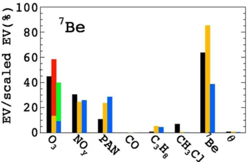
tion in the simulated7Be mean concentration is found (435 and 234 fCi/SCM for the observations and model, respectively). Figure 3 shows the7Be factor profiles when the measurements with [O3]>100 ppbv are included. The results are similar to Fig. 2. The

scaled EV of O₃for the model (green bar) is lower because the observed O₃variability is higher.

15

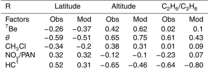
We examine the factor correlations with latitudes, altitude, and C2H6/C3H8 ratio in

order to further investigate the factor characteristics (Table 1). The higher C₂H₆/C₃H₈ ratio reflects photochemically aged air masses (Wang and Zeng, 2004). The positive correlations of the7Be factor with altitude (r=0.42 and 0.62 for the observed and sim-ulated datasets, respectively) are expected for a factor dominated by transport from

20

the stratosphere. The weak negative correlations with latitude (r=−0.26 and −0.37) indicate that stratosphere-troposphere exchange is likely more active at lower latitudes in 40–60◦N region.

The potential temperature (θ) factor has large variability of θ (77% and 36.4 K for the observations, 95% and 26.8 K for the model). It explains 14% of observed O3

vari-25

ability (3.6 ppbv) and 12.8% of simulated O3 variability (3.1 ppbv). The negative factor

correlations with latitude (r=−0.59 and −0.51 for the observed and simulated datasets, 15504

(12)

ACPD

Full Screen / Esc

respectively) and CO (r=−0.64 and −0.52, respectively, not shown in the table), and positive correlations with altitudes (r=0.65 and 0.75, respectively) and C2H6/C3H8ratio

(r=0.61 and 0.43, respectively) imply that this factor is likely associated with intercon-tinental long-range transport of O₃ from lower latitudes, which is consistent with the result by Wang et al. (2003b).

5

The CH3Cl factor is characterized by large signals of CH3Cl (78% and 41.2 pptv

for the observations, 95% and 25.1 pptv for the model), and no O₃ variability is ex-plained by this factor. This factor contains significant CO variability, which can imply the biomass burning influence. However, the very small factor correlations with C2H6/C3H8

ratio (r=0.01 and 0.09), and negative correlation with latitude (r=−0.34 and −0.2) may

10

support the large biogenic CH₃Cl emissions from the tropics (e.g., Yoshida et al., 2004, 2006) rather than biomass burning.

The NOy/PAN factor has large signals of NOy (44% and 120 pptv for the

tions, 74% and 160 pptv for the model) and PAN (68% and 96.3 pptv for the observa-tions, 45% and 63.4 pptv for the model). This factor is the second important factor for

15

tropospheric O3 variability at mid latitudes (25.6% and 6.6 ppbv for the observations,

18.4% and 4.4 ppbv for the model). It correlates positively with latitude (r=0.32 and 0.32 for the observed and simulated datasets, respectively). The correlations with al-titude (r=−0.12 and −0.1) and C2H6/C3H8ratio (r=−0.23 and 0.07) are much weaker

compared to the hydrocarbon factor discussed below, implying that the factor

repre-20

sents long-range transport of reactive nitrogen.

The hydrocarbon factor is characterized by large variability of CO (48% and 26.8 ppbv for the observations, 54% and 21.3 ppbv for the model) and C₃H₈(90% and 360 pptv for the observations, 90% and 272 pptv for the model). There is no contribu-tion to tropospheric O3variability. It positively correlates with latitude (r=0.52 and 0.31

25

for the observed and simulated datasets, respectively). Clear negative correlations with altitudes (r=−0.65 and −0.46, respectively) and C2H6/C3H8 ratio (r=−0.64 and

−0.8, respectively) reflect the influence of relatively fresh emissions from the surface at higher latitude in 40–60◦N region (Table 1).

(13)

ACPD

Full Screen / Esc

3.1.2 TOPSE at high latitudes

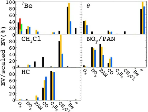
Five factors are identified for high latitudes (7Be, θ, CH3Cl, NOy/PAN, and

hydrocar-bons; Fig. 4). As mid latitudes, there is also significant difference in 7Be variability between observations and simulation (415 fCi/SCM and 206 fCi/SCM, respectively) in the 7Be factor, reflecting serious underestimation of 7Be by GEOS-Chem. Liu et

5

al. (2001) artificially scaled down the stratospheric 7Be source by a factor of ∼3 in order to adjust for some surface measurements of 7Be. However, the simulated 7Be mean concentrations and the variability accounted for in the 7Be factor show consis-tent underestimations by about a factor of 2 in TOPSE and TRACE-P (to be shown) datasets. It implies that the factor of 3 reduction in the stratospheric7Be source in the

10

standard GEOS-Chem model is too large.

The7Be factor shows comparable O3variabilities between observations and

simula-tion (34% and 13.7 ppbv for the observasimula-tions, 45% and 12.4 ppbv for the model). The stratospheric O3 fraction from the tagged O3 simulation suggests that∼70% is of the

stratospheric origin (Fig. 4). The tropospheric fraction is∼30% in this factor. The

pos-15

itive correlations with altitude (r=0.48 and 0.4, respectively) and negative correlations with CO (r=−0.41 and −0.38, not shown in the table) support its stratospheric origin (Table 2).

The potential temperature (θ) factor shows large variabilities of θ (77% and 29 K for the observations, 98% and 32.6 K for the model). Its contributions to O3 levels are

20

as much as that of the7Be factor (39% and 15.4 ppbv for the observations, 41% and 10.7 ppbv for the model), which is different from mid latitudes. The positive correlation with altitude (r=0.51 and 0.55, respectively) and C2H6/C3H6 ratio (r=0.22 and 0.4,

respectively) indicates that this factor is likely associated with transport of reactive-nitrogen poor air masses from lower latitudes. Tagged O3 simulation shows that O3

25

variability accounted for in this factor is produced in the troposphere (orange bar). The CH3Cl factor is characterized by large signals of CH3Cl (78% and 38.6 pptv for

the observations, 98% and 20.3 pptv for the model), but its contribution to O3variability

(14)

ACPD

Full Screen / Esc

is insignificant. This factor is positively correlated with altitude (r=0.38 and 0.46 for the observed and simulated datasets, respectively), which is consistent with long-range transport of high CH3Cl air masses since there are no significant sources of CH3Cl at

high latitudes.

The NO_y/PAN factor has large signals of NO_y (60% and 135 pptv for the

observa-5

tions, 57% and 119 pptv for the model) and PAN (72% and 132 pptv for the observa-tions, 62% and 67.5 pptv for the model). This factor also has clear chemical signals of CO but not7Be, implying that the air masses are influenced by industrial/fossil fuel emissions at high latitudes (Table 2). This factor, however, contributes to less than 5% of O3 variability, reflecting the largely inactive photochemical environment at high

10

latitudes in spring (Wang at al., 2003a).

The hydrocarbon factor is characterized by a large variability of CO (40% and 12.2 ppbv for the observations, 62% and 22.5 ppbv for the model) and C3H8(90% and

314 pptv for the observations, 88% and 297 pptv for the model). It does not contribute to tropospheric O3 variability. Just as mid latitudes, the negative correlations with

al-15

titude (r=−0.43 and −0.49, respectively) and C2H6/C3H8 ratio (r=−0.77 and −0.79,

respectively) reflect air masses affected by relatively fresh emissions (Table 2).

3.1.3 Springtime O3trends at northern mid and high latitudes

Understanding the contributions to the seasonal O3trend is another important purpose

of this study. As stated in Sect. 2.1, this study analyzed only eight tracers due to the

lim-20

ited availability of simulated tracers, while the previous study (Wang et al., 2003b, here-after referred to as the previous study) included fourteen tracers with seven factors. At mid latitudes, the seasonal increase of all factors of measurements is 6.48 ppbv/month (Table 3), consistent with the previous study (6.3 ppbv/month). The largest contributor to the O3 seasonal trend is the NOy/PAN factor (3.55 ppbv/month, Table 3) followed

25

by the7Be factor (2.66 ppbv/month). That is also consistent with the previous study (3.5 ppbv/month, and 2.5 ppbv/month, respectively). In contrast, the simulated overall

(15)

ACPD

Full Screen / Esc

seasonal increase is only 3.01 ppbv/month, indicating a large underestimation. The in-crease from the NOy/PAN factor is underestimated (1.32 ppbv/month in the model), and

the7Be factor increase is also much smaller than that of observation (1.29 ppbv/month in the model).

At high latitudes, the overall springtime increase from the measurements is

5

4.29 ppbv/month (Table 3), comparable with the previous study (4.6 ppbv/month). In comparison, the simulated increase is only 1.3 ppbv/month, indicating a significant un-derestimation. The most contributions to the seasonal increases at high latitudes are from7Be, θ, and NOy/PAN factors (1.78, 1.16, and 1.10 ppbv/month, respectively) in

the measurement dataset. In comparison, the corresponding trends in the model are

10

much lower (0.76, 0.77, and 0.11 ppbv/month). The underestimation is particularly large for the NOy/PAN factor, implying that simulated O3production in reactive-nitrogen

rich air masses does not increase as much as in the observations. The negative O₃ trend in the hydrocarbon factor in the simulation but not in the measurements is a likely reflection of the problematic simulations of its major components (C2H6 and C3H6) in

15

May by GEOS-Chem (Wang and Zeng, 2004).

The NOy/PAN factor trend is consistent with the previous study. However, the

contributions of 7Be and θ factors are different from those of the previous study (0.8 ppbv/month and 0.6 ppbv/month, respectively). The previous study had additional tracers resulting in the CH4-halocarbon factor. It accounts for transport from lower

20

latitudes, which contributes to the largest increase of O3at 1.7 ppbv/month at high

lati-tudes. In this study, that large increase trend is apportioned into the7Be and θ factors since we do not have CH4 and halocarbon (other than CH3Cl) simulations in

GEOS-Chem. Because the PMF factor projections are for the same number of tracers, model results can still be evaluated in this analysis. The CH₄-halocarbon factor contribution

25

to O3variability is, however, <10% (3 ppbv) at high latitudes in the previous study; thus

the effect of the missing factor on factor apportioned O3 variability is fairly insignificant

in this study.

During TOPSE, the major contributions to the seasonal O3increase in springtime is

(16)

ACPD

Full Screen / Esc

from intercontinental transport of polluted air masses, while the major contributions to O₃ variability is from the stratospheric influences and long-range transport of O₃ from lower latitudes. While the model generally captures the factor contributions to O3, factor

contributions to the springtime increasing trend of O3in the measurements are severely

underestimated. These model underestimations are also consistent with the results by

5

Wang et al. (2006). Improvements in the seasonal transitions of cross-tropopause and intercontinental transport are needed in the model.

3.2 TRACE-P

The TRACE-P experiment was conducted to investigate the effects of Asian outflow to the Pacific during spring (Jacob et al., 2003). As mentioned in Sect. 2.1, the

TRACE-10

P results are biased toward the middle and upper troposphere (more than 40% of the data is above 7 km). Compared to TOPSE analysis, there are fewer coincident measurements limited mostly by the availability of7Be measurements (65 and 79 for mid and low latitudes, respectively). We analyze the datasets for low (15–30◦) and mid (30–45◦) latitudes separately.

15

3.2.1 TRACE-P at mid latitudes

Four factors are identified for mid latitudes (7Be, θ, CH3Cl, and NOy/hydrocarbons,

Fig. 5). The7Be factor shows larger O₃variability in the observations than model re-sults (68% and 20.8 ppbv for the observations, 48.5 % and 13.8 ppbv for the model). There is also a large underestimation in simulated 7Be variability (428 fCi/SCM and

20

211 fCi/SCM, respectively) for the reason discussed in Sect. 3.1.2. The tagged O₃ simulation shows that∼80% of O3variability in this factor is of the stratospheric origin.

While this factor in the simulated dataset showed a positive correlation with altitude (r=0.63), it has a much weaker correlation (r=0.12) in the measurements (Table 4). One possible reason for the large difference is that transport from the stratosphere

oc-25

(17)

ACPD

Full Screen / Esc

the stratosphere-troposphere exchange occurs in regions farther away, further down-ward transport or mixing with low-altitude polluted air would reduce the gradients in altitude.

The potential temperature (θ) factor shows large signals of θ (87% and 26.3 K for the observations, 93% and 23.4 K for the model). The factor correlations in Table 4

char-5

acterize this factor as long-range transport of air masses from the tropics (r=0.79 and 0.67 with altitude for the observed and simulated datasets, respectively; and r=0.86 and 0.82 with C₂H₆/C₃H₈ ratio, respectively). While this factor accounts for 25.6% of O3 variability in the simulated datasets, it has no contribution in the measurement

dataset.

10

The CH₃Cl factor is characterized by the large signals of CH₃Cl (76% and 37.4 pptv for the observations, 95% and 42.2 pptv for the model). The contributions of this fac-tor to O3 variability are small in measured and simulated datasets. The significant

contributions to CO (65% and 74.5 ppbv for the observations, 38% and 26.6 ppbv for the model), negative correlations with altitude (r=−0.25 and −0.77, respectively) and

15

C2H6/C3H8ratio (r=−0.33 and −0.6 for the observed and simulated datasets,

respec-tively), and the reactive nitrogen signals suggest a strong influence from biomass burn-ing. This factor contributes to NOy vaiability (168 pptv) only in the simulated dataset,

and PAN variability (164 pptv) only in the observed dataset. Since PAN is an impor-tant component of NO_y, the signal in PAN will propagate to become a signal of NO_y.

20

However, another large component of NOy is HNO3, which can be removed rapidly by

wet deposition in the atmosphere. It appears to suggest that the scavenging of HNO3

(a major component of NO_y) during transport and the production of PAN from biomass burning NOxare underestimated by the model. The stronger negative correlation of the

factor with altitude suggests that the altitude of biomass burning transport is lower in

25

the model. This model bias also leads to a higher negative correlation with C₂H₆/C₃H₈ as is found here because mixing with locally emitted C2H6 and C3H8tends to destroy

the negative correlation.

In TRACE-P analysis, the NO_y/PAN and hydrocarbon factors in TOPSE are com-15510

(18)

ACPD

Full Screen / Esc

bined (now NO_y/hydrocarbon factor) because the separation of those factors leads to incomparable factor profiles between the measurements and model results. The NOy/hydrocarbon factor is characterized by a large variability of NOy(51% and 509 pptv

for the observations, 67% and 523 pptv for the model), PAN (40% and 195 pptv for the observations, 72% and 234 pptv for the model), CO (25% and 27.8 ppbv for the

ob-5

servations, 53% and 54.6 ppbv for the model), and C3H8 (78% and 335 pptv for the

observations, 87% and 461 pptv for the model). This factor shows a contribution to tropospheric O3variability only in the simulation (14.5%). This factor has negative

cor-relations with altitudes (r=−0.77 and −0.31 for the observed and simulated datasets, respectively) and C₂H₆/C₃H₈ratio (r=−0.64 and −0.16, respectively), likely reflecting

10

relatively the influence of fresh industrial/fossil fuel emissions over Asia (Table 4). The stronger negative correlations with C2H6/C3H8ratio and altitude in the measurements

than the simulations imply that mixing is too fast at low altitudes in the model.

3.2.2 TRACE-P at low latitudes

Four factors also are identified for low latitudes (7Be, θ, CH₃Cl, and NOy/hydrocarbons,

15

Fig. 6). The 7Be factor shows smaller O3 variability in the measurements than the

model simulation (17.4% and 7.1 ppbv for the observations, and 30.8% and 9.9 ppbv for the model). Large underestimation by a factor of 3 is found in simulated7Be variability (411 fCi/SCM and 139 fCi/SCM for the observed and simulated datasets, respectively). There are no data with O3above 100 ppbv in both observations and simulation results

20

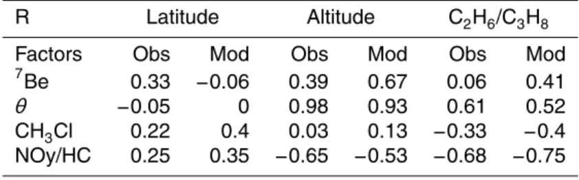
at low latitudes. The stratospheric O₃ fraction from the tagged O₃ simulation shows that∼50% is due to transport from the stratosphere, which is the smallest stratospheric influence among the datasets. The positive factor correlations with altitude (r=0.39 and 0.67, respectively) reflect in part the contribution from the stratosphere (Table 5). The weaker correlations with altitude and C2H6/C3H8 ratio in the observed than simulated

25

datasets likely reflect either a problem in the transport locations from the stratosphere or the mixing between stratospheric and tropospheric air masses in the model.

(19)

ACPD

Full Screen / Esc

the observations, 77% and 23.2 K for the model). While the7Be factor is the largest contributor to simulated O3 variability at low latitudes, the θ factor is the largest

con-tributor to observed O₃variability (27.4% and 11.1 ppbv for the observations, and 21% and 6.7 ppbv for the model). The model estimates a small stratospheric fraction of 15% in this factor. This factor contains small signals of simulated NOy, PAN, and CO,

5

which are absent in the observed dataset, indicating again that mixing of different air masses in the model is overestimated. The correlation coefficients are more consis-tent between observed and simulated datasets for this factor. The positive correlations with altitude (r=0.98 and 0.93 for the observed and simulated datasets, respectively) and C₂H₆/C₃H₈ratio (r=0.61 and 0.52, respectively) and negative correlations with CO

10

(r=−0.66 and −0.49, not shown in the table) suggest the dominance of photochemi-cally aged upper tropospheric air in this factor.

The CH₃Cl factor is characterized by large signals of CH₃Cl (81% and 39.7 pptv for the observations, 67% and 42 pptv for the model) and a significant contribution to O3 variability is found in this factor (24.6% and 9.9 ppbv for the observations, 15.7%

15

and 5 ppbv for the model). This factor contributes more to O₃ in the observations than the model. The larger contribution in the observations is associated with CO (50% and 40.7 ppbv), NOy (53.7 pptv), and PAN (52 pptv). In comparison, this factor

in the simulated dataset has a smaller contribution from CO (22% and 17.4 ppbv) and negligible contributions from NOyand PAN. The observed profile is consistent with the

20

characteristics of biomass burning.

It appears that the contributions to PAN, NO_y, and CO from biomass burning are attributed to the NOy/hydrocarbon factor in the model. Comparing the profiles between

CH3Cl and NOy/hydrocarbon factors, a major separation factor between these factors

is the correlation between C₃H₈ and CH₃Cl. In both datasets, almost all the C₃H₈

25

signals are in the NOy/hydrocarbon factor. There is no correlation between C3H8and

CH3Cl in the observed dataset. Consequently there is no CH3Cl signal in the observed

NO_y/hydrocarbon factor. The opposite is true in the simulated dataset, leading to a significant contribution to the CH3Cl variability (29% and 17 pptv). The inadequate

(20)

ACPD

Full Screen / Esc

separation of C₃H₈ and CH₃Cl in the model may result from two sources. The first is that mixing is overestimated in the model, which results in excessive mixing of biomass burning and industrial/urban air masses. The second is that the locations of biomass burning or industrial/urban sources are misplaced in the model, which also leads to unrealistic mixing.

5

The NOy/hydrocarbon factor is characterized by large variabilities of NOy (33% and

185 pptv for the observations, 60% and 376 pptv for the model), PAN (30% and 56.5 pptv for the observations, 55% and 94.3 pptv for the model), CO (40% and 34.2 ppbv for the observations, 57% and 49.6 ppbv for the model), and C3H8(85% and 172 pptv

for the observations, 75% and 234 pptv for the model). The factor contributions to

10

these trace gases are lower in the observations than the model results because some of the enhancements in the model are due in part to biomass burning emissions. In-terestingly, the factor contributions to tropospheric O3 variability are comparable in the

observations (16% and 6.5 ppbv) and model results (18.5% and 6 ppbv) even though the enhancements in NOy, PAN, and CO are higher in the model results. The two

15

datasets have comparable positive factor correlations with latitude (r=0.25 and 0.35 respectively), and large negative correlations with altitude (r=−0.65 and −0.53, re-spectively) and C2H6/C3H8 ratio (r=−0.68 and −0.75, respectively) indicating fresh

pollution plumes from East Asia.

4 Discussion and conclusions

20

Trace gas measurements of TOPSE and TRACE-P experiments are analyzed with the PMF method in order to evaluate the model performance in simulating source contri-butions to tropospheric O₃variability and its springtime increase (during TOPSE). We select a suite of relatively long-lived variables, which are available both in observations and GEOS-Chem model: seven chemicals (O3, NOy, PAN, CO, C3H8, CH3Cl, and

7

Be)

25

and one dynamic tracer (potential temperature). The evaluation has a bias towards a high altitude of 5–8 km (∼70% of the data) for TOPSE and 7–12 km (∼50% of the data)

(21)

ACPD

Full Screen / Esc

for TRACE-P, due to the availability of7Be measurements.

In general, the factor loadings between the observations and simulations are in better agreement during the TOPSE experiment than TRACE-P. The former experiment took place in remote regions. Therefore, the model results are not as sensitive to source locations as for the latter experiment. There are also slightly more data points

(deter-5

mined largely by the availability of7Be measurements) in the former experiment. We summarize the factor contributions to O3variability in Figs. 7 and 8.

The7Be factor is found in all regions. Among all the factors, the largest discrepancy is found in the variability of7Be, which is controlled largely by its source in the strato-sphere. The simulated results are a factor of 2–3 lower than those observed. The large

10

underestimation is due to the default reduction of the stratospheric7Be source by a factor of ∼3 in the model. Inadvertently, the default reduction provides a test for the PMF analysis.

Tagged O3 simulations in the model indicate that the O3 signal in the 7

Be factor is controlled largely (70–80%) by transport from the stratosphere at mid and high

lati-15

tudes. Only over the lower latitude does the stratospheric contribution drop to∼50%. The 7Be factor explains 34–40% of O3 variability in the measurement dataset

dur-ing TOPSE, in agreement with the simulated dataset. Durdur-ing TRACE-P, this factor contributes 68% and 17% at mid and low latitudes, respectively in the measurement dataset. In comparison, the contributions in the simulated datasets are also higher

20

at mid latitudes (49%) and lower at low latitudes (31%). In general, we find that the decrease of stratospheric O₃ contributions (and the increase of tropospheric O₃ con-tributions) from mid to low latitudes during TRACE-P are much larger in the measured than simulated datasets. One potential reason is that mixing is overestimated between mid and low latitudes in the model, reducing the gradients between the two latitude

25

bands.

Another common factor is the θ factor. There are consistent positive correlations of this factor with altitude and C₂H₆/C₃H₈ ratio, indicating long-range transport in the upper troposphere. The contribution of this factor to reactive nitrogen is small,

(22)

ACPD

Full Screen / Esc

flecting likely chemical aging during transport. The large contribution to O₃ variability at high latitudes during TOPSE (∼40%) in the measurement dataset is in agreement with the simulated dataset. In comparison, its contributions to mid latitudes during TOPSE are much lower in both datasets. During TRACE-P, there is no contribution from this factor to O3variability in the measurement dataset at mid latitudes. However,

5

26% contribution is found in the simulated dataset. A similar situation is found for the NO_y/hydrocarbon factor. Excessive mixing between mid and low latitudes could explain some of the discrepancy. Further, the unresolved portion of O3 variability is ∼30% in

this case, much higher than the range of 11–19% in the other cases. Some of the unresolved portion is due to O₃production in the troposphere.

10

A third common factor found is the CH₃Cl factor. The contributions of this factor to O3are usually small. The exception is at low latitudes during TRACE-P, when biomass

burning contributes to both CH3Cl and O3. Some of the biomass burning contribution

in the simulated datasets is attributed to the NO_y/hydrocarbon factor since simulated C3H8is correlated with CH3Cl. The latter correlation was not found in the measurement

15

dataset. Thus, we combine the CH3Cl and NOy/hydrocarbon factor contributions to O3

variability; it is somewhat higher in the measurement dataset (41%) than the simulated dataset (34%). As discussed previously, the difference can be reduced if mixing is reduced between mid and low latitudes in the model.

During TOPSE, the NO_y/PAN factor is resolved separately from the hydrocarbon

fac-20

tor. The latter made no contribution to O3variability. The NOy/PAN factor contributions

are much higher at mid latitudes (18–26%) than high laitutdes (<5%) in measured and simulated datasets, reflecting more active photochemistry at mid latitudes in spring.

Since the TOPSE experiment last longer than TRACE-P, we compare the factor con-tributions to the seasonal trend of O3 in the observed and simulated datasets.

De-25

spite of reasonably good agreements in the averaged contributions, the trends of factor contributions are quite different. The observed springtime O3 increase is higher than

simulated by a factor 2 at mid latitudes (6.5 vs. 3 ppbv/month) and a factor of 3 at high latitudes (4.3 vs. 1.3 ppbv/month). The increasing trend from the stratospheric

(23)

contri-ACPD

Full Screen / Esc

bution (the7Be factor) is underestimated by a factor of 2. The increasing trend from the tropospheric contribution is simulated well for the θ factor. However, the increasing trend from O₃ production by reactive nitrogen (the NO_y/PAN factor) is underestimated by a factor of >3 (3.5 ppbv/month vs. 1.3 ppbv/month at mid latitudes and 1 ppbv/month vs. 0.1 ppbv/month at high latitudes). These results suggest that more attention needs

5

to be placed on improving the simulations of the temporal trends of trace gases in chemical transport models.

Acknowledgements. This work was supported by the National Science Foundation Atmo-spheric Chemistry Program. The GEOS-CHEM model is managed at Harvard University with support from the NASA Atmospheric Chemistry Modeling and Analysis Program.

10

References

Atlas, E. L., Ridley, B. A., and Cantrell, C.: Tropospheric Ozone Production about the Spring Equinox (TOPSE) Experiment: Introduction, J. Geophys. Res., 108(D4), 8353, doi:10.1029/2002JD003172, 2003.

Benkovitz, C. M., Schwartz, C. E., Jensen, M. P., et al.: Global gridded inventories of

an-15

thropogenic emissions for sulfur and nitrogen, J. Geophys. Res., 101(D22), 29 239–29 253, 1996.

Berntsen, T. K., Karlsdo’ttir, S., and Jaffe, D. A.: Influence of Asian emissions on the compo-sition of air reaching the northwestern United States, Geophys. Res. Lett., 26, 2171–2174, 1999.

20

Bey, I., Jacob, D. J., Yantosca, R. M., et al.: Global modeling of troposheric chemistry with assimilated meteorology: Model description and evaluation, J. Geophys. Res., 106, 23 073– 23 096, 2001.

Chameides, W. L., Davis, D. D., Rodgers, M. O., et al.: Net ozone photochemical production over the eastern and central north Pacific as inferred from CTE/CITE 1 observations during

25

fall 1983, J. Geophys. Res., 92, 2131–2152, 1987.

Chen, P.: Isentropic cross-tropopause mass exchange in the extratropics, J. Geophys. Res., 100, 16 661–16 673, 1995.

(24)

ACPD

Full Screen / Esc

Chin, M., Jacob, D. J., Munger, J. W., et al.: Relationship of ozone and carbon monoxide over North America, J. Geophys. Res., 99, 14 565–14 573, 1994.

Dibb, J. E., Meeker, L. D., Finkel, R. C., et al.: Estimation of stratospheric input to the Arctic troposphere: 7Be and 10Be in aerosols at Alert, Canada, J. Geophys. Res, 99, 12 855– 12 864, 1994.

5

Dibb, J. E., Talbot, R. W., Scheuer, E., et al.: Stratospheric influence on the northern North American free troposphere during TOPSE:7Be as a stratospheric tracer, J. Geophys. Res., 108(D4), 8363, doi:10.1029/2001JD001347, 2003.

Duncan, B. N., Martin, R. V., Staudt, A. C., et al.: Interannual and seasonal variability of biomass burning emissions constrained by satellite observations, J. Geophys. Res., 108(D2),

10

4100, doi:10.1029/2002JD002378, 2003.

Fishman, J. and Seiler W.: Correlative nature of ozone and carbon monoxide in the tropo-sphere: Implications for the tropospheric ozone budget, J. Geophys. Res., 88, 3662–3670, 1983.

Holton, J. R., Haynes P. H., McInyre E. M., et al.: Stratosphere-troposphere exchange, Rev.

15

Geophys, 33, 403–439, 1995.

Jacob, D. J., Logan, J. A., and Murti, P. P.: Effect of rising Asian emissions on surface ozone in the United States, Geophys. Res. Lett., 26, 2175–2178, 1999.

Jacob, D. J., Crawford, J. H., Kleb, M. M., et al.: Transport and Chemical Evolution over the Pacific (TRACE-P) aircraft mission: Design, execution, and first results, J. Geophys. Res.,

20

108(D20), 1–19, 2003.

Jaffe, D., Anderson, T., Covert, D., et al.: Transport of Asian air pollution to North America, Geophys, Res. Lett., 26, 711–714, 1999.

Lee, E., Chan, C. K., and Paatero, P.: Application of positive matrix factorization in source ap-portionment of particulate pollutants in Hong Kong, Atmos. Environ., 33, 3201–3212, 1999.

25

Liu, H., Jacob, D. J., Bey, I., and Yantosca, R. M.: Constraints from210Pb and 7Be on wet deposition and transport in a global three-dimensional chemical tracer model driven by as-similated meteorological fields, J. Geophys. Res., 106, 12 109–12 128, 2001.

Liu, H., Jacob, D. J., Chan, L. Y., et al.: Sources of tropospheric ozone along the Asian Pa-cific Rim: An analysis of ozonesonde observations, J. Geophys. Res., 107(D21), 4573,

30

doi:10.1029/2001JD002005, 2002.

Liu, H., Jacob, D. J., Dibb, J. E., Fiore, A. M., et al.: Constraints on the sources of tropospheric ozone from 210Pb-7Be-O₃ correlations, J. Geophys. Res., 109, D07306,

(25)

ACPD

Full Screen / Esc

doi:10.1029/2003JD003988, 2004.

Liu, S. C., Trainer, M., Fehsenfeld, F. C., et al.: Ozone production in the rural troposphere and the implications for regional and global ozone distributions, J. Geophys. Res., 92, 4191– 4207, 1987.

Liu, W., Wang, Y., Russell, A., et al.: Atmospheric aerosols over two urban-rural pairs in

south-5

eastern United States: Chemical composition and sources, Atmos. Environ., 39, 4453–4470, 2005.

Logan, J. A.: Tropospheric ozone: Seasonal behavior, trends, and anthropogenic influence, J. Geophys. Res., 90, 10 463–10 482, 1985.

Mauzerall, D. L., Narita, D., Akimoto, H., et al.: Seasonal characteristics of tropospheric ozone

10

production and mixing ratios over East Asia: A global three dimensional chemical transport model analysis, J. Geophys. Res., 105, 17 895–17 910, 2000.

Olivier, J. G. J. and Berdowski, J. J. M.: Global emissions sources and sinks, in: The Climate System, edited by: Berdowski, J., Guicherit, R., and Heij, B. J., A. A. Balkema Publish-ers/Swets and Zeitlinger Publishers, Lisse, The Netherlands, ISBN 90-5809-255-0, 33–78,

15

2001.

Oltmans, S. J. and Levy II., H.: Seasonal cycle of surface ozone over the western North Atlantic, Nature, 358, 392–394, 1992.

Paatero, P. and Tapper, U.: Positive Matrix Factorization: a non-negative factor model with optimal utilization of error estimates of data values, Environmetrics, 5, 111–126, 1994.

20

Paatero, P.: Least squares formulation of robust non-negative factor analysis, Chemomet. Intell. Lab. Sys., 37, 23–35, 1997.

Paatero, P., Hopke, P. K., Song, X.-H., et al.: Understanding and controlling rotations in factor analytic models, Chemomet. Intell. Lab. Sys., 60, 253–264, 2002.

Parrish, D. D., Holloway, J. S., Trainer, M., et al.: Export of North American ozone pollutions to

25

the North Atlantic Ocean, Science, 259, 1436–1439, 1993.

Penkett, S. A. and Brice, K. A.: The spring maximum in photo-oxidants in the Northern Hemi-sphere tropoHemi-sphere, Nature, 319, 655–657, 1986.

Shim, C., Wang, Y., Singh, H. B., et al.: Source characteristics of oxygenated volatile organic compounds and hydrogen cyanide, J. Geophys. Res., 112, D10305,

30

doi:10.1029.2006JD007543, 2007.

Tanimoto, H., Wild, O., Kato, S., et al.: Seasonal cycles of ozone and oxidized nitrogen species in northeast Asia: 2. A model analysis of the roles of chemistry and transport, J. Geophys.

(26)

ACPD

Full Screen / Esc

Res., 107(D23), 4706, doi:10.1029/2001JD001497, 2002.

Wang, Y., Jacob, D. J., and Logan, J. A.: Global simulation of tropospheric O₃-NO_X -hydrocarbon chemistry, 3. origin of troposheric ozone and effects of non-methane hydro-carbons, J. Geophys. Res., 103, 10 757–10 767, 1998b.

Wang, Y., Liu, S. C., Wine, P. H., et al.: Factors Controlling Tropospheric O₃, OH, NO_x, and

5

SO₂over the Tropical Pacific during PEM-Tropics B, J. Geophys. Res., 106, 32 733–32 748, 2001.

Wang, Y., Ridley, B., Fried, A., et al.: Springtime photochemistry at northern mid and high latitudes, J. Geophys. Res., 108(D4), 8358, doi:10.1029/2002JD002227, 2003a.

Wang, Y., Shim, C., Blake, N., et al.: Intercontinental transport of pollution manifested in the

10

variability and seasonal trend of springtime O₃ at northern middle and high latitudes, J. Geophys. Res., 108(D21), 4683, doi:10.1029/2003JD003592, 2003b.

Wang, Y. and Zeng, T.: On tracer correlations in the troposphere: The case of ethane and propane, J. Geophys. Res., 109, D24306, doi:10.1029/2004JD005023, 2004.

Wang, Y., Choi, Y. S., Zeng, T., et al.: Late-spring increase of trans-Pacific pollution transport

15

in the upper troposphere, Geosphys. Res. Lett., 33, L01811, doi:10.1029/2005GL024975, 2006.

Wild, O. and Akimoto, H.: Intercontinental transport of ozone and its precursors in a three-dimensional global CTM, J. Geophys. Res., 106, 27 729–27 744, 2001.

Yoshida, Y., Wang, Y. H., Zeng, T., et al.: A three-dimensional global model study of

20

atmospheric methyl chloride budget and distributions, J. Geophys. Res., 109, D24309, doi:24310.21029/2004JD004951, 2004.

(27)

ACPD

Full Screen / Esc

Printer-friendly Version Interactive Discussion Table 1. The factor scores correlations (r) with latitude, altitude, and C₂H₆/C₃H₈ for TOPSE

mid latitudes.

R Latitude Altitude C₂H₆/C₃H₈ Factors Obs Mod Obs Mod Obs Mod

7 Be −0.26 −0.37 0.42 0.62 0.02 0.1 θ −0.59 −0.51 0.65 0.75 0.61 0.43 CH₃Cl −0.34 −0.2 0.38 0.31 0.01 0.09 NO_y/PAN 0.32 0.32 −0.12 −0.1 −0.23 0.07 HC1 0.52 0.31 −0.65 −0.46 −0.64 −0.80

Extreme factor scores (outside 2σ range) and the measurements that have O₃ greater than 100 ppbv are excluded.1HC denotes the hydrocarbon factor.

(28)

ACPD

Full Screen / Esc

Printer-friendly Version Interactive Discussion Table 2. Same as Table 1, but for TOPSE high latitudes.

7 Be −0.08 −0.08 0.48 0.4 0.25 0.11 θ −0.1 −0.2 0.51 0.55 0.22 0.4 CH₃Cl −0.07 −0.2 0.38 0.46 0.18 −0.18 NO_y/PAN 0.16 0.07 0.02 −0.34 0.25 −0.14 HC1 −0.08 0.04 −0.43 −0.49 −0.77 −0.79

(29)

ACPD

Full Screen / Esc

Printer-friendly Version Interactive Discussion Table 3. Factor contributions to O₃seasonal increase (ppbv/month) for TOPSE.

Mid latitudes High latitudes Obs Mod Obs Mod

7 Be 2.7 1.3 1.8 0.8 θ 0.3 0.4 1.2 0.8 CH₃Cl 0 0 0.3 0 NO_y/PAN 3.5 1.3 1.1 0.1 HC 0 0 0 −0.4 Total 6.5 3.0 4.3 1.3 Only the measurements O₃<100 ppbv are analyzed.

(30)

ACPD

Full Screen / Esc

Printer-friendly Version Interactive Discussion Table 4. Same as Table 1, but for TRACE-P mid latitudes.

7

Be −0.37 0.05 0.12 0.63 0.32 0.28 θ −0.33 −0.67 0.79 0.67 0.86 0.82 CH₃Cl −0.02 0.11 −0.25 −0.77 −0.33 −0.6 NO_y/HC 0.18 −0.42 −0.77 −0.31 −0.64 −0.16

(31)

ACPD

Full Screen / Esc

Printer-friendly Version Interactive Discussion Table 5. Same as Table 1, but for TRACE-P low latitudes.

7 Be 0.33 −0.06 0.39 0.67 0.06 0.41 θ −0.05 0 0.98 0.93 0.61 0.52 CH₃Cl 0.22 0.4 0.03 0.13 −0.33 −0.4 NOy/HC 0.25 0.35 −0.65 −0.53 −0.68 −0.75 15524

(32)

ACPD

Full Screen / Esc

Printer-friendly Version Interactive Discussion Fig. 1. Locations of aircraft measurements.

(33)

ACPD

Full Screen / Esc

Printer-friendly Version Interactive Discussion Fig. 2. Explained variation (%, defined in Sect. 2.2) profiles of the observed (shown in black)

and simulated datasets (shown in yellow and red) at mid latitudes (40–60◦N) during TOPSE. Also shown is the scaled EV profiles (in blue and green) for the simulated datasets for di-rect comparison with the measurements (Eq. (4), see text for details). The two-color bars for O₃ show the model simulated stratospheric (upper bar, red or green) and tropospheric (lower bar, yellow or blue) fractions. The results are for measurement data with O₃ concentrations <100 ppbv (and the corresponding model dataset).

(34)