Effects of spatial variability of precipitation for process-orientated hydrological modelling: results from two nested catchments

HAL Id: hal-00298620

https://hal.archives-ouvertes.fr/hal-00298620

HAL is a multi-disciplinary open access

archive for the deposit and dissemination of sci-entific research documents, whether they are pub-lished or not. The documents may come from teaching and research institutions in France or abroad, or from public or private research centers.

L’archive ouverte pluridisciplinaire HAL, est destinée au dépôt et à la diffusion de documents scientifiques de niveau recherche, publiés ou non, émanant des établissements d’enseignement et de recherche français ou étrangers, des laboratoires publics ou privés.

Effects of spatial variability of precipitation for

process-orientated hydrological modelling: results from

two nested catchments

D. Tetzlaff, U. Uhlenbrook

To cite this version:

D. Tetzlaff, U. Uhlenbrook. Effects of spatial variability of precipitation for process-orientated hy-drological modelling: results from two nested catchments. Hydrology and Earth System Sciences Discussions, European Geosciences Union, 2005, 2 (1), pp.119-154. �hal-00298620�

HESSD

Full Screen / Esc

Print Version Interactive Discussion

Hydrol. Earth Syst. Sci. Discuss., 2, 119–154, 2005 www.copernicus.org/EGU/hess/hessd/2/119/ SRef-ID: 1812-2116/hessd/2005-2-119 European Geosciences Union

Hydrology and Earth System Sciences Discussions

E

ffects of spatial variability of

precipitation for process-orientated

hydrological modelling: results from two

nested catchments

D. Tetzlaff1and U. Uhlenbrook2

1

Department of Geography and Environment, University of Aberdeen, Aberdeen AB24 3UF, Scotland, United Kingdom

2

Institute of Hydrology, University of Freiburg, Fahnenbergplatz, 79098 Freiburg, Germany Received: 14 December 2004 – Accepted: 17 January 2005 – Published: 19 January 2005 Correspondence to: D. Tetzlaff (d.tetzlaff@abdn.ac.uk)

HESSD

Full Screen / Esc

Print Version Interactive Discussion Abstract

The importance of considering the spatial distribution of rainfall for process-oriented hydrological modelling is well-known. However, the application of rainfall radar data to provide such detailed spatial resolution is still under debate. In this study the process-oriented TACD (Tracer Aided Catchment model, Distributed) model had been used to 5

investigate the effects of different spatially distributed rainfall input on simulated dis-charge and runoff components on an event base. TACD is fully distributed (50×50 m2 raster cells) and was applied on an hourly base. As model input rainfall data from up to 11 ground stations and high resolution rainfall radar data from an operational C-band radar were used. For seven rainfall events the discharge simulations were investigated 10

in further detail for the mountainous Brugga catchment (40 km2) and the St. Wilhelmer Talbach (15.2 km2) sub-basin, which are located in the Southern Black Forest Moun-tains, south-west Germany. The significance of spatial variable precipitation data was clearly demonstrated. Dependent on event characteristics, localized rain cells were oc-casionally poorly captured even by a dense ground station network, and this resulted 15

in insufficient model results. For such events, radar data can provide better input data. However, an extensive data adjustment using ground station data is required. There-fore, a new method was developed that considers the rainfall intensity distribution. The use of the distributed catchment model allowed further insights into spatially variable impacts of different rainfall estimates. Impacts for discharge predictions are the largest 20

in areas that are dominated by the production of fast runoff components. To conclude, the improvements for distributed runoff simulation using high resolution rainfall radar input data are strongly dependent on the investigated scale, the event characteristics, the existing monitoring network and, last but not least, the applied model.

HESSD

Full Screen / Esc

Print Version Interactive Discussion 1. Introduction

The spatial variability of rainfall is often termed as the major source of error in inves-tigations of rainfall-runoff processes and modelling (O’Loughlin et al., 1996; Syed et al., 2003). Especially for smaller catchments and for runoff processes that respond directly to precipitation detailed rainfall information is necessary (Woods et al., 2000). 5

However, the spatial variability of precipitation can be very strong. The mean diame-ter of a rain cell has been estimated between 15 km (Luyckx et al., 1998) and one to five kilometres (Woods et al., 2000) or an area of 1–2 km2(Thomas et al., 2003), and such cells can move significantly during events. Obviously, such detailed information on rainfall distribution and heterogeneity is unobtainable with a standard ground station 10

density of 1 station per 20 km2(Michaud and Sooroshian, 1994).

In addition to errors in catchment precipitation – due to the spatial aggregation of rainfall information (Faures et al., 1995; Winchell et al., 1998) – relatively small di ffer-ences in catchment precipitation based on different rainfall input data might result in comparable large errors in simulated runoff (Sun et al., 2000). Using spatially high 15

resolution rainfall input data, some studies have found an increase of simulated runoff volumes (Michaud and Sorooshian 1994; Winchell et al., 1998), while one study found a decrease (Faures et al., 1995). Krajewski et al. (1991) have shown a higher sensitivity of catchment runoff response with respect to the temporal than to the spatial resolu-tion of precipitaresolu-tion data. Obled et al. (1994) have found no significant improvement in 20

hydrological predictions using temporally higher distributed rainfall in a medium-sized rural catchment, although they emphasised the possibility of contradictory results for smaller urbanized or larger rural catchments.

The spatial and temporal distribution of precipitation can have different relevance for distinct runoff generation processes. Winchell et al. (1998) have found that modelled 25

Hortonian runoff generation was more influenced by spatially and temporally averag-ing of precipitation than saturation excess runoff. Hortonian overland flow increased with a more detailed rainfall input. Also Michaud and Sorooshian (1994) have found

HESSD

Full Screen / Esc

Print Version Interactive Discussion

an increase of Hortonian overland flow using spatially more detailed rainfall informa-tion. Furthermore, different spatio-temporal variable characteristics of rain cells, e.g. storm cell position or volume of the storm core, cause different impacts to runoff gen-eration mechanism dependent on catchment and event characteristics (Syed et al., 2003). In addition to runoff volume and peak flow, also the timing is influenced by 5

spatial distribution of rainfall input (Krajewski et al., 1991; Ogden et al., 2000). Sun et al. (2000) improved the timing of peak flow estimations using higher distributed rainfall data. However, improvements of flow predictions depend on a wide range of factors such as investigated catchment scale, rainfall and catchment characteristics, runoff generation mechanism and applied model (Ogden et al., 2000; Arnaud et al., 2002). 10

Rainfall radar data provide the opportunity to apply spatially distributed rainfall data in distributed catchment modelling. Especially in catchments with coarse raingauge networks, radar data can be helpful for distributed runoff simulations (Michaud and Sorooshian, 1994; Lange et al., 1999; Woods et al., 2000). Although in recent years rainfall radar data have been utilized more and more in hydrological studies, the benefit 15

of radar data is still discussed controversially. There exist a number of studies which focus, for example, on descriptions of rain drop size distribution, variability in Vertical Profile Reflectivity (VPR) or other influencing factors if transferring measured reflectiv-ities in rainfall intensreflectiv-ities (Smith and Krajewski, 1993; Fabry, 1997; Borga et al., 1997; Hirayama et al., 1997; Uijlenhoet and Sticker, 1999; Grecu and Krajewski, 2000a, b; 20

Borga, 2002). These authors developed techniques for an improved estimation of rain-fall rates from radar reflectivities for hydrological application and thus, an improvement of runoff modelling, although they acknowledge that significant uncertainties remain. A relatively large uncertainty, which is associated with rainfall intensities estimated from reflectivities, affects mainly the magnitude of rainfall graphs (Morin et al., 2001). Op-25

erational available data are in most cases not sufficient enough regarding their quality due to the single-polarization measurement. There are only few studies, which apply approaches with an acceptable expense in correction of the radar data (Winchell et al., 1998; Ogden et al., 2000; Carpenter et al., 2001).

HESSD

Full Screen / Esc

Print Version Interactive Discussion

The study has three specific aims: Firstly, to develop a methodology for an optimum adjustment of the operational available radar data for single events for a subsequent hydrological model application. Secondly, to investigate the influence of different rain-fall data sources on the estimation of catchment precipitation. Thirdly, to examine the influence of different spatially distributed rainfall inputs on simulated runoff and different 5

runoff components at the event scale in two nested catchments. To explore these ques-tions, two nested, meso-scale catchments in the Southern Black Forest Mountains, Germany, were investigated, that are equipped with a dense rainfall station network and a weather radar.

2. Materials and methods

10

2.1. Study site

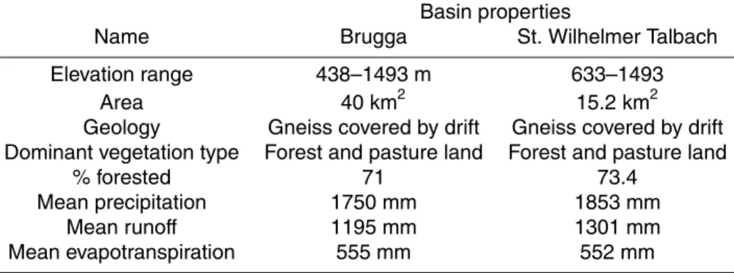
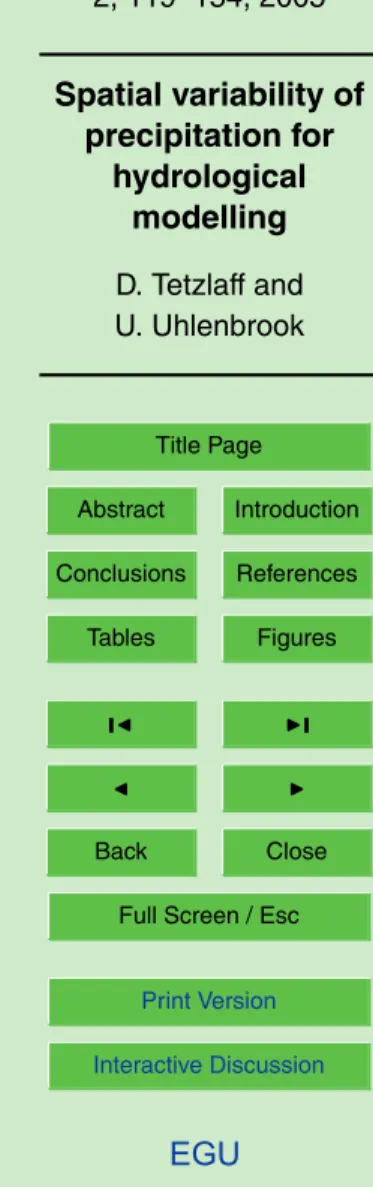
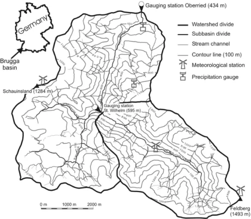
The study was performed in the mesoscale Brugga catchment (40 km2) and its sub-catchment St. Wilhelmer Talbach (15.2 km2) located in the Southern Black Forest Mountains, southwest Germany (Fig. 1, Table 1). The Brugga basin is a pre-alpine mountainous catchment with a mean elevation of about 986 m a.s.l. The mountainous 15

part of the basin is characterized by steep hillslopes, bedrock outcrops, deeply incised and narrow valleys, and gentler areas at the mountaintops. The gneiss bedrock is cov-ered by brown soils, debris and drift of varying depths at the hillslopes (0–10 m). Soil hydraulic conductivity is generally high: the infiltration capacity is too high to generate infiltration excess except in little settlements. The morphology is characterised by mod-20

erate to steep slopes (75% of the area), hilly hilltops and hilly uplands (about 20%), and narrow valley floors (less than 5%). The overall average slope is 19◦, calculated with a 50×50 m2digital elevation model.

The mean precipitation amount is 1750 mm per year; mean runoff is 1195 mm. Mean daily flow is comparable with 39.1 l s−1km−2 (Brugga) and 41.3 l s−1km−2 (St. 25

HESSD

Full Screen / Esc

Print Version Interactive Discussion

of 840 l s−1 km−2 (Brugga) and 763 l s−1km−2 (St. Wilhelmer Talbach) (Table 1). Due to the strong variability of elevation, slope and exposition caused by the deeply in-cised valleys the catchment is characterised by a large heterogeneity of all climate elements, in particular precipitation. This causes spatially and temporally irregular elevation-precipitation gradients within the basin and articulated luv-lee i.e. rain shadow 5

effects.

Experimental investigations using artificial and natural tracers showed the impor-tance of three main flow systems (Uhlenbrook et al., 2002; 2004a): (i) fast runoff com-ponents (surface and near-surface runoff) which are generated on sealed or saturated areas or, additionally, on steep highly permeable slopes covered by boulder trains; 10

(ii) slow base flow components (deep groundwater) are connected with fractured rock aquifers and the deeper parts of the weathering zone, and (iii) an intermediate flow system originates mainly from (peri-) glacial deposits of the slopes (shallow ground water). These are mainly delayed runoff components compared to the surface and near-surface runoffs. However, they can also contribute to flood formation depending 15

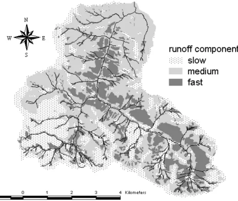
on the antecedent moisture content. A simplified spatial delineation of hydrological homogeneous regions – generating predominately the three main runoff components base flow, interflow as well as surface and near surface runoff – is shown in Fig. 2. Most parts of the test sites are covered by glacial and periglacial drift cover and hence, influenced by interflow processes. The extent of areas generating mainly fast runoff 20

components is defined by saturated and sealed areas as well as very steep hillslopes (>25◦).

2.2. Precipitation data

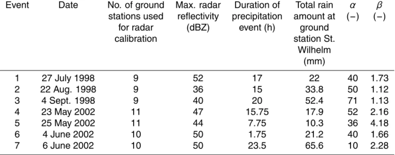
Seven single rain events were investigated with measured maximum radar reflectivities of up to 52 dBZ (Table 3). Due to the contrasts in event characteristics, event 6 and 7 25

are mainly presented and discussed within this study. Event 6 is the most convective event with very short duration and high rainfall intensities. Event 7 shows the highest

HESSD

Full Screen / Esc

Print Version Interactive Discussion

precipitation amount but over a much longer duration causing the highest flow.

The rainfall radar data used in this study are measured with a C-band Doppler radar with a wavelength of 3.75–7.5 cm and one elevation angle (0.5◦). The rainfall radar station is located near the highest point of the Brugga catchment at the peak of the Feldberg Mountain (Fig. 1). The radar product is a quantitative DX product provided by 5

the German Weather Service (DWD). The spatial resolution is 1 km×1◦azimuth angle with a temporal resolution of 5 min. The data from 1998 have only dBZ classes with 4-dBZ steps due to a systematic measuring error during this time period. These technical problems were solved in 1999 and from then the resolution of dBZ values is 0.5.

The radar data were corrected for clutters by the German Weather Service using 10

clutter maps. These clutter maps are compiled during a period when no precipitation echoes are relevant. There were neither distance nor vertical reflectivity profiles cor-rections conducted. A detailed description of the used DX product can be found at DWD (1997). Problems connected with these operational radar products available in Germany are discussed e.g. in Quirmbach (2003).

15

For radar data calibration, up to 11 ground stations were – event dependent – avail-able within and nearby the catchment boundaries (Tavail-able 3; Fig. 1). Nine of these ground stations are located in a circumference of maximal 30 km of the investigated catchments at elevations between 200 and 1010 m a.s.l. More ground stations within the catchments are available but they are measuring on a much coarser resolution and 20

were not used for radar data calibration. But for the subsequent runoff simulations, in addition to the radar data, up to seven ground stations, located within or very close to the Brugga basin were used. Basin precipitation was estimated using an 80:20 combi-nation of the inverse distance weighting (IDW) method (80%) and an elevation gradient (20%) to consider the spatial variability of basin precipitation. The IDW method is often 25

used as an alternative to Kriging when there are insufficient data to compute the rain-fall covariance function (Odgen et al., 2000). The IDW method calculates a weighted average precipitation for each raster cell with a weight of d−2, while d is the distance between the rain station and the respective raster cell. Only stations within a radius

HESSD

Full Screen / Esc

Print Version Interactive Discussion

of 6 km for each raster cell were considered for the calculation. The elevation gradient is a non-linear function that considers the mean annual increase of precipitation with height (Uhlenbrook et al., 2004b). This gradient was kept constant within the basin, but varied for every modelling time step.

The precipitation for each raster cell and time step was calculated as weighted aver-5

age (80:20) of the two regionalization methods. Therefore the value obtained from the elevation was weighted with 20% and the value obtained from the IDW method was weighted with 80%. This was done because of an observed elevation dependence of precipitation that was found for longer time intervals (monthly, yearly), but which was not always observed for shorter time steps in the mountainous test site. During storms 10

the location of the rain cell is more important than elevation. Consequently, the used re-gionalisation scheme is a compromise to capture the spatial distribution during shorter time intervals but also to reproduce the long term pattern. The precipitation measure-ment error caused by wind was corrected according to the approach of Schulla (1997) that differentiates between liquid and solid precipitation.

15

2.3. Radar data adjustment methods

Weather radars are not measuring the rainfall intensity itself but the radar reflectivity. Reflectivities are converted into rainfall rates using the Z/R-relation

Z = α ∗ Rβ <=> R = (Z/α)1/β = (10d BZ/10/α)1/β (1) with

20

d BZ = 10 log Z, (2)

where Z is the reflectivity (mm6m−3) and R the rain intensity (mm h−1). α and β are fitting parameters.

The calculation of intensities from the measured reflectivities is influenced by numer-ous factors and includes high uncertainties (Uijlenhoet and Stricker, 1999). Reflectiv-25

HESSD

Full Screen / Esc

Print Version Interactive Discussion

characteristics. Therefore, different Z/R-relations arise according to seasonal and me-teorological conditions (Smith and Krajewski, 1993; Quirmbach et al., 1999; Haase and Crewell, 2000). For the correction of radar data there exist two main basic approaches. The first is the correction of vertical profiles of reflectivities using different radar beam elevation angles (e.g. Andrieu et al., 1997; Creutin et al., 1997; Borga, 2002). The 5

radar data used in this study were measured only with one elevation angle. Therefore this approach could not be applied. Additionally, it can be assumed that – especially during convective events – small variabilities of reflectivities occur until a height where the 0◦C isotherm is reached (Fabry, 1997). In summer, this border lies some kilometres above ground. Furthermore, variations of reflectivities are small near the certain radar 10

site (Andrieu and Creutin, 1995). Both aspects, that radar data of convective events were used and for a study catchment close to the radar site let the authors assume that the reflectivity profiles can be neglected in this case study.

Therefore, the second approach based on the adjustment of radar-derived precip-itation using gauge data was applied. The aim of such approach is to correct the 15

estimated radar precipitation to the quantity of gauge measurements (Adamowski and Muir, 1989; Seo et al., 1999; Sun et al., 2000; Vallabhaneni et al., 2002). A main error source in such radar data calibration is due to the drawback on appropriate ground sta-tion data (Ciach and Krajewski, 1999). Ground stasta-tion data can capture the temporal distribution of rainfall very well, but the spatial representation is often limited, espe-20

cially in heterogeneous catchments with spare ground station network. In contrast, radar data allow very detailed information about the spatial distribution of precipitation, but measurements have practical limitations in estimating rainfall totals.

2.4. Applied rainfall-runoff model TACD

In recent years, several hydrological models have been used at the Brugga basin and 25

sub-basins (e.g. PRMS/MMS, Mehlhorn and Leibundgut 1999; TOPMODEL, G ¨untner et al., 1999; HBV, Uhlenbrook et al., 1999). The application of these models and the results of the experimental studies led to the development of the TAC model, the Tracer

HESSD

Full Screen / Esc

Print Version Interactive Discussion

Aided Catchment model (Uhlenbrook and Leibundgut 2002). The aim was to develop a better process-realistic model to compute the water balance on a daily mode. TAC is a process-oriented, semi-distributed catchment model, which requires a spatial delin-eation of units with the same dominating runoff generation processes (cf. hydrotopes or hydrological response units).

5

The TAC model was advanced to the TACD model (TAC, distributed), a fully dis-tributed raster model (Uhlenbrook et al., 2004b). The spatial division was undertaken by delineating the catchment into units sharing the same dominating runoff generation processes. The units were converted into 50×50 m2raster cells that are connected by a single flow algorithm. Channel routing is modelled with a kinematic wave approach 10

(implicit, non-linear). The whole model is integrated into the GIS PC-Raster (Karssen-berg et al., 2001).

The TACD model was applied to the Brugga basin using the period 1 August 1995– 31 July 1996 for model calibration (further details are given in Uhlenbrook et al., 2004b). It was initialised over a period of three months, which had some fillings 15

of the different hydrological storages prior this period. The calibrated parameter set was used for modelling the St. Wilhelmer Talbach sub-basin without re-calibration. To evaluate model goodness the model efficiency R_eff(Q) (−) (Nash and Sutcliffe, 1970) and the model efficiency using logarithmic runoff values R_eff(log Q) (−) were used. Good simulation results were obtained at Brugga catchment for the model calibra-20

tion period (R_eff(Q)=0.94; R_eff(log Q)=0.99) and validation period (three years record; R_eff(Q)=0.80; R_eff(log Q)=0.83) after a split-sample test. A multiple-response validation using different kind of additional data, including tracer data, demonstrated the process-realistic basis of the model with its simulated runoff components (Uhlenbrook et al., 2004b).

25

The calibrated radar data with a temporal resolution of 5 min were aggregated to 1 h intervals to serve as input for the TACD model. The original spatial resolution of the polar co-ordinate grid of 1 km×1◦azimuth angle was disaggregated to a 50×50 m2grid using an algorithm devised by Lange (2003, pers. com.). Due to technical limitations

HESSD

Full Screen / Esc

Print Version Interactive Discussion

of the radar measurement, a small area around the radar device needed to be “filled” with ground data measurements.

The following methodology was conducted to compare the impact of the two precip-itation inputs on event runoff simulations. The model was run twice, each time with the same initialisation period (eight months), parameter values (determined during model 5

calibration) and input data sets, but with different basin precipitation maps for each time-step of the investigated events. This has the advantage that the model runs con-tinuously and thus the spatial and temporal variable soil moisture and groundwater storages are modelled reasonably before the investigated event. This is a prerequisite for process-oriented modelling, which could not have been fulfilled if the events were 10

modelled separately and independently from the previous hydrological conditions.

3. Results

3.1. Radar data calibration at the event scale

Within this study, radar data were calibrated using the certain radar bin corresponding to the ground station data. Firstly, equal time intervals of 5 min between the radar and 15

ground data were constructed for comparability of both data sets. Therefore, an event and station dependent time shift correction between the both data sets was necessary. Results showed that between both data sets a station and event dependent time shift correction of 5 to 15 min was necessary. Because of wind drift of falling precipitation a neighbouring pixel can be more representative than the direct corresponding pixel. 20

Thus an average of nine cells, i.e. the cell with the location of the rain gauge and all eight surrounding cells, was used as radar point data. Depending on event and station, a coefficient of determination (r2) between both data sets of more than 0.47 was obtained after time shift correction. Additionally, a visual check was executed to identify errors in the radar images e.g. ground clutters.

25

min-HESSD

Full Screen / Esc

Print Version Interactive Discussion

imum square deviation method for the cumulative curves of both data sets (Fig. 3). By minimising the square deviation between the cumulative precipitation curves of both data sets, the distribution of rainfall intensities in each time step is considered. An additional objective was to minimise the difference between the total precipitation amounts of both data sets. An optimum parameter set of α and β of the Z/R-relation 5

for each event was determined by automatically minimising both square deviation and differences of total rain amounts of all available ground stations. Optimum, but phys-ically reasonable α and β parameters were then determined. This non-linear adjust-ment avoids weighting higher rain intensities more significantly than lower rain intensi-ties. Resulting Z/R-relations differ strongly between the single events (Table 3). In a 10

next step, the measured radar reflectivities were transformed into rainfall intensities us-ing spatially averaged but event dependent Z/R-relations. Usus-ing these Z/R-relations the radar intensities were calculated for the whole catchment in a spatial resolution of 1 km×1◦azimuth angle and a temporal resolution of 5 min using Arc Info GIS routines. The exemplary shown percentage deviations between the total rain amounts at the 15

respective ground station and the corresponding radar bin for events 6 and 7 show clearly that there was neither systematically under- nor overestimation of the precipi-tation amount (Table 4). Occasionally, at single sprecipi-tations high deviations occur, but at station 7, which is situated near the centre of the St. Wilhelmer Talbach sub-catchment, the deviations can be neglected (<10%).

20

3.2. Influence of different rainfall input data on the estimated catchment rainfall To examine the influence of different rainfall input data for basin precipitation, mean, maximum and minimum precipitation values were compared (Table 5). It becomes clear that the maximum and minimum values were more extreme – i.e. higher and lower – using radar data than ground station data. The high maximum values using 25

IDW-elevation method for event 7 were due to a high value at only one ground station (Feldberg), while all other ground stations recorded in precipitation amounts between 60–70 mm during this event. Although maximum intensities were higher with radar

HESSD

Full Screen / Esc

Print Version Interactive Discussion

data, in most cases mean catchment precipitation was higher using the IDW-elevation regression compared to radar data. This overestimation is caused by the regionaliza-tion of the precipitaregionaliza-tion values of certain ground staregionaliza-tions to large areas of the basin.

Using the different precipitation inputs caused large differences in the spatial delin-eation of the precipitation fields (Fig. 4). During the strong convective event 6 (du-5

ration: 1.75 h) the rain cell was mainly located in the St. Wilhelmer Talbach subcatch-ments (Fig. 4a), which is well represented by one ground station. The precipitation field with radar data was much more heterogeneous than with the IDW-elevation-regression method with precipitation ranges between 1 mm (minimum) and 38 mm (maximum) within the whole Brugga catchment. Due to the interpolation of rainfall mean precip-10

itation was 30% higher using the IDW-elevation-regression method than radar data, although maximum rainfall intensities were not captured using just ground station data. Event 7 (Fig. 4b) was less convective, but with higher total rain amounts after a longer event duration (23.5 h). Again, maximum and minimum values (Table 5) were more extreme with radar data compared to application of ground station data and the 15

precipitation field using radar data was more heterogeneous compared to the IDW-elevation-regression method, although differences in the total amounts were compen-sated because of the longer duration of the event. Again, higher total precipitation amounts were reached applying ground station data, which caused mean precipitation values 17% higher than with radar data.

20

3.3. Influence of different rainfall input on simulated discharge

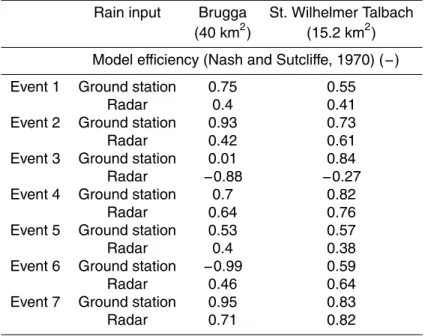
Subsequently, the ground station data and the calibrated radar data were used as input for runoff simulation using TACD. For all investigated events model efficiency values (Table 6) can be used for an assessment of the influence of different spatially distributed rainfall input on simulated runoff. In general, better simulation results – 25

i.e. higher model efficiencies (Nash and Sutcliffe, 1970) – were gained using ground station data and in the smaller St. Wilhelmer Talbach catchment. It has to be noted that this catchment is relatively well covered by one ground station located near its centre.

HESSD

Full Screen / Esc

Print Version Interactive Discussion

For some events (e.g. event 3) model efficiency values were insufficient, regardless of which rainfall input was used. In most cases the percentage deviation of the simulated from the observed peak discharge was less using ground station data. Neither type of input data resulted in a systematically under- or overestimation of peak discharge. For the St. Wilhelmer Talbach sub-catchment, results were less clear regarding one 5

input resulting in better runoff simulations. In the Brugga catchment, there was also no clear pattern that one rain input resulted in better simulation results than the other regarding discharge volume. But volumes in the Brugga catchment were more often overestimated, while in the St. Wilhelmer Talbach catchment they were more often underestimated.

10

Looking in further detail to the two contrasting events, it becomes clear that during event 6 the use of ground station data resulted in an overestimation of the simulated peak discharge of 52% compared with the observed hydrograph in the Brugga catch-ment (Fig. 5). Simulation with spatial higher resolution radar data resulted in an over-estimation of only 17%. The discharge volumes were overestimated by 38% (ground 15

station data) and 22% (radar data).

For interpretation of the hydrographs, it is important to consider the spatial distribu-tion of precipitadistribu-tion in combinadistribu-tion with the spatial delineadistribu-tion of the main hydrological response units (Fig. 2). The higher calculated catchment precipitation amount espe-cially in the North of the Brugga catchment – due to the transformation of single ground 20

station values for the whole sub-basin – resulted in this large overestimation in runoff simulation using ground station data. The effect was reinforced because this strong overestimation occurs in large parts of the sub-catchment where fast runoff compo-nents are dominant (see Fig. 2). Model efficiencies for ground station data simulation were poor (R_eff=−0.99), but much better with radar data (R_eff=0.46). In this catchment, 25

for which there are little ground station data, the use of radar data especially during such a highly localised event produced better runoff simulation results. If too high pre-cipitation is determined in areas where fast runoff components are dominant, the errors in runoff simulation can be substantial.

HESSD

Full Screen / Esc

Print Version Interactive Discussion

The simulations in the St. Wilhelmer sub-catchment produced with both types of rain-fall input data comparable results for event 6 (Fig. 6). Both rainrain-fall data sets resulted in a slight peak and volume overestimation compared to the observed discharge, although there was no volume error using ground station data. For peak discharge, deviations are less and also model efficiency values are higher using radar data which can be 5

explained again by a better capturing of precipitation characteristics for areas with fast runoff response.

During event 7 all model performance parameters were poorer using radar data as rainfall input compared to ground station data for the Brugga catchment. These simu-lation results were caused by an underestimation of the catchment precipitation during 10

this event in this basin, although during calibration there was no systematic underes-timation of the rain amount using radar data (Table 4). For this less localised event with the longer duration the main influencing factor for runoff simulation was the total difference between both rainfall data sets. Spatial distribution of rainfall in combination with runoff generation patterns is of less relevance. Thus, the simulated hydrograph 15

using ground station data fitted much better with the observed hydrograph (Fig. 5). For the St. Wilhelmer Talbach catchment model efficiency values for event 7 are good with R_eff>0.8 for both data sets. Peak discharge and volume are overestimated with ground station data (33% and 15%, respectively) but underestimated with radar data (−19% and −18%, respectively, Fig. 6).

20

4. Discussion and conclusion

The operational available radar data in Germany which were used in this study are only corrected for ground clutters by the provider. As such, no information about e.g. vertical reflectivity profiles are available for those data. The efforts necessary for cor-rections using ground station data by the user are high (Quirmbach, 2003) and the 25

quality and the use of such data for hydrological application is limited. The developed method is based on the adjustment of radar-derived precipitation using gauge data and

HESSD

Full Screen / Esc

Print Version Interactive Discussion

considers the intensity distribution within the certain event in adjusting the cumulative curves of both data sets. As the intra-storm variability of rainfall intensity is considered explicitly using this approach, ground station data at high temporal resolution have to be applied for a reasonable comparison with the radar data. For radar calibration, not only ground stations within the catchment boundary but also those within a radius of 5

not more than 20 km were used to extend the data set and to capture a wider spectrum of rainfall intensities. This method was developed for an event-based calibration. But also for non-event based hydrological modelling radar data can be calibrated using this methodology, because periods without rain don not have to be calibrated. Calibration efforts can thus be minimized.

10

The use of radar data resulted in higher maximum and lower minimum precipitation when the spatial distribution of the rainfall within the catchment was compared with ground data. The use of ground station data resulted also in much smoother precip-itation patterns due to the regionalization of point rainfall information to large areas. However, mean values of basin precipitation were in most cases higher using ground 15

station data. In the larger catchment shorter, convective events lead to higher di ffer-ences in catchment precipitation (i.e. total amount and spatial distribution) between both types of rainfall data. It is more unlikely that localised rain cells are captured by the available ground station net. Such differences in either extreme values or total rain amounts can have crucial effects for subsequent hydrological modelling (e.g. Michaud 20

and Sorooshian, 1994). In addition, Syed et al. (2003) have found that the position of the storm core relative to the outlet becomes more important for runoff simulation with increasing catchment size.

Using spatially higher resolution rainfall data some authors found an increase in runoff volume (e.g. Michaud and Sorooshian 1994). However, Faures et al. (1995) 25

emphasised a decrease. Even if in this study two rainfall data types were compared and not just different spatial resolutions of one data type, the changes in model results cannot be neglected. Within this study 41% of the investigated cases resulted in an increase in runoff volume using radar data. In 53% of the cases volumes were higher

HESSD

Full Screen / Esc

Print Version Interactive Discussion

using less spatially distributed ground station data. Deviations in peak discharge were also less using ground station data. But here two rainfall data types were compared and not only different spatial resolutions of one data type. Thus, errors might be caused already during data calibration.

Generally, for evaluations about the goodness of simulation results based on certain 5

precipitation input various model performance values should be used to capture the whole spectrum of effects. There were no clear patterns obvious that one rainfall input resulted in better simulations than the other. For example, for the highly convective event (event 6) errors in runoff simulation were less if spatially high resolution radar data were applied. This was obvious by the much better model efficiency values and 10

fewer deviations in both peak discharge and discharge volume for both catchments. Particularly in parts of the basin which are characterised by fast runoff response the correct detection of the rainfall pattern using highly distributed radar data was impor-tant. But in most investigated cases model efficiencies were poorer and percentage deviations were higher using radar data.

15

For single events with a longer duration, the spatial distribution of precipitation in-fluences less the mean catchment precipitation because differences in rainfall are more balanced. The differences in precipitation might be balanced or smoothed by the non-linear response runoff generation processes, especially in mesoscale catch-ments. Hence, differences in precipitation might not result in the same degree of differ-20

ences in the simulated hydrographs. In smaller catchments differences in distribution of the precipitation have a much larger influence on the runoff simulation because less averaging-out of precipitation differences within the catchment is possible.

In general, the use of distributed, process-oriented models allows the use of detailed information and complex data sets, and the analysis of many details in hydrological 25

predictions. However, the effects of the detailed information for any runoff modelling system need to be understood and the additional data set needs to be utilized ade-quately by the applied model. Then also the effects of different input data on many model outputs (e.g. the changing contribution of runoff components) can be analysed.

HESSD

Full Screen / Esc

Print Version Interactive Discussion

In this study it was demonstrated clearly that the rainfall overestimation can have sub-stantial impact for the flood prediction especially if such overestimation occurs in areas which are dominated by the formation of fast runoff components. Consequently, the importance of the input data for flood prediction can be very large, and this should be considered as much as the nowadays frequently discussed parameter uncertainty 5

when using such process-orientated models.

Acknowledgements. The detailed radar data have been provided from the German Weather

Service (DWD). The State Institute for Environmental Protection Baden-W ¨urttemberg (Lan-desanstalt f ¨ur Umweltschutz (LfU) Baden-W ¨urttemberg) made the precipitation ground station data available (special thanks to M. Bremicker). In addition, the federal environmental

sur-10

vey (Umweltbundesamt, UBA) provided the rainfall data from the station Schauinsland. The Gew ¨asserdirektion Waldshut, Germany, measured the runoff data. The input of G. G¨assler during the analysis of the radar data and during extensive discussions is gratefully acknowl-edged. Many thanks to J. Lange (University of Freiburg, Germany), who has provided a code for converting the radar data. Parts from the converting program from J. Lange were combined

15

with a reading program from D. Sacher (J. Lang Datenservice). Thanks to D. Sacher, too.

References

Adamowski, K. and Muir, J.: A Kalman-filter modelling of space-time rainfall using radar and raingauge observations, Canadian J. Civil Engineering, 16, 5, 767–773, 1989.

Andrieu, H., Creutin, J. D., Delrieu, G., and Faures, D.: Use of weather radar for the hydrology

20

of mountainous area, Part I: radar measurement interpretation, J. Hydrol., 193, 1–4, 1–25, 1997.

Andrieu, H. and Creutin, J. D.: Identification of vertical profiles of radar reflectivities for hydrolog-ical applications using inverse method, Part 1: Formulation, J. Appl. Meteor., 34, 225–239, 1995.

25

Arnaud, P., Bouvier, C., Cisneros, L., and Dominquez, R.: Influence of spatial variability on flood prediction, J. Hydrol., 260, 216–230, 2002.

Borga, M.: Accuracy of radar rainfall estimates for streamflow simulation, J. Hydrol., 267, 26– 39, 2002.

HESSD

Full Screen / Esc

Print Version Interactive Discussion Borga, M., Da Ros, D., Fattorelli, S., and Vizzaccaro, A.: Influence of various weather radar

correction procedures on mean areal rainfall estimation and rainfall-runoff simulation, In: Weather radar technologies for water resources management, edited by Braga, B. J. and Massambani, O., IRTCUD/University of Sao Paulo, Brazil and IHP-UNESCO, 1997.

Carpenter, T. M., Georgakakos, K. P., and Sperfslagea: On the parametric and NEXRAD-radar

5

sensitivities of a distributed hydrologic model suitable for operational use, J. Hydrol., 253, 169–193, 2001.

Ciach, G. J. and Krajewski, W.: On the estimation of radar rainfall error variance, Adv. Wat. Resour., 22, 6, 585–595, 1999.

Creutin, J. D., Andrieu, H., and Faures, D.: Use of weather radar for the hydrology of a

moun-10

tainous area, Part II: radar measurement validation, J. Hydrol., 193, 26–44, 1997.

DWD (Deutscher Wetterdienst, German Wheather Service): AKORD – Anwenderkoordinierte Organisation von Radar-Daten. Produktkatalog (product catalogue), Deutscher Wetterdienst Gesch ¨aftsfeld Hydrometeorologie, Offenbach Germany, 1997.

Fabry, F.: Vertical profiles of reflectivity and precipitation intensity, In: Weather radar

tech-15

nologies for water resources management, edited by Braga, B. J. and Massambani, O., IRTCUD/University of Sao Paulo, Brazil and IHP-UNESCO, 1997.

Faures, J.-M., Goodrich, D. C., Woolhiser, D. A., and Sorooshian, S.: Impact of smale-scale spatial rainfall variability on runoff modelling, J. Hydrol., 173, 309–326, 1995.

Grecu, M. and Krajewski, W.: Simulation study of the effects of model uncertainty in variational

20

assimilation of radar data on rainfall forecasting, J. Hydrol., 239, 1–4, 85–96, 2000a.

Grecu, M. and Krajewski, W.: A large-sample investigation of statistical procedures for radar-based short-term quantitative precipitation forecasting, J. Hydrol., 239, 1–4, 69–84, 2000b. G ¨untner, A., Uhlenbrook, S., Seibert, J., and Leibundgut, C.: Multi-criterial validation of

TOP-MODEL in a mountainous catchment, Hydrol. Processes, 13, 1603–1620, 1999.

25

Haase, G. and Crewell, S.: Simulation of radar reflectivities using a mesoscale weather forecast model, Wat. Resour. Res., 36, 8, 2221–2231, 2000.

Hirayama, D., Fujita, M., and Nakatsugawa, M.: The identification of optimum Z-R relation based on runoff analysis, In: edited by Braga, B. J. and Massambani, O., Weather radar technologies for water resources management, IRTCUD/University of Sao Paulo, Brazil and

30

IHP-UNESCO, 1997.

Karssenberg, D., Burrough, P.A., Sluiter, R., and de Jong, K.: The PCRaster software and course materials for teaching numerical modelling in the environmental sciences,

Transac-HESSD

Full Screen / Esc

Print Version Interactive Discussion tions in GIS, 5, 2, 99–110, 2001.

Krajewski, W. F., Ventakataramann, L., Georgakakos, K. P., and Jain, S. C.: A Monte Carlo study of rainfall sampling effect on a distributed catchment model, Wat. Resour. Res., 27, 1, 119–128, 1991.

Lange, J., Leibundgut, C., Greenbaum, N., and Schick, A. P.: A non-calibrated rainfall-runoff

5

model for large, arid catchments, Wat. Resour. Res., 35, 7, 2161–2172, 1999.

LfU (Landesanstalt f ¨ur Umweltschutz Baden-W ¨urttemberg):

Hochwasserabfluss-Wahrscheinlichkeiten in Baden-W ¨urttemberg, Oberirdische Gew ¨asser/Gew ¨asser ¨okologie, 54, Karlsruhe, 1999.

Luyckx, G., Willems, P., and Berlamont, J.: Influence of the spatial variability of rainfall on sewer

10

systems design, Proceedings of the British hydrological society international conference, Exeter, UK, 1998.

Mehlhorn, J. and Leibundgut, C.: The use of tracer hydrological time parameters to calibrate baseflow in rainfall-runoff modelling, IAHS-Pub. No. 258, 119–125, 1999.

Michaud, J. D. and Sorooshian, S.: Effects of rainfall-sampling errors on simulations of desert

15

flash floods, Wat. Resour. Res., 30, 10, 2765–2775, 1994.

Morin, E., Enzel, Y., Shamir, U., and Garti R.: The characteristic time scale for basin hydrologi-cal response using radar data, J. Hydrol., 252, 85–99, 2001.

Nash, J. E. and Sutcliffe, J. V.: River flow forecasting through conceptual models, 1. A discus-sion of principles, J. Hydrol., 10, 282–290, 1970.

20

O’Loughlin, G., Huber, W., and Chocat, B.: Rainfall-runoff processes and modelling, J. Hydraul. Res., 34, 6, 733–751, 1996.

Obled, C., Wendling, J., and Beven, K.: The sensitivity of hydrological models to spatial rainfall patterns: an evaluation using observed data, J. Hydrol., 159, 305–308, 1994.

Ogden, F. L., Sharif, H. O., Senarath, S. U. S., Smith, J. A., Baeck, M. L., and Richardson, J.

25

R.: Hydrologic analysis of the Fort Collins, Colorado, flash flood of 1997, J. Hydrol., 228, 82–100, 2000.

Quirmbach, M.: Nutzung von Wetterradardaten f ¨ur Niederschlags- und Abflussvorhersagen in urbanen Einzugsgebieten (Use of wheater radar for rainfall-runoff forecasting in urban catchments), PhD Thesis, Ruhr-Universit ¨at Bochum, Bochum, 178, 2003.

30

Quirmbach, M., Schultz, G., and Frehmann, T.: Use of weather radar for combined control of an urban drainage system and a sewage treatment plant, Impacts of urban growth on surface water and groundwater quality (Proceedings of IUGG 99 Symposium HS5, Birmingham, July

HESSD

Full Screen / Esc

Print Version Interactive Discussion 1999), IAHS Publ., 245–250, 1999.

Schulla, J.: Hydrologische Modellierung von Flußeinzugsgebieten zur Absch ¨atzung der Folgen von Klima ¨anderungen (Hydrological modelling of river basins for evaluating the impacts of climatic changes), Z ¨uricher Geographische Hefte, 65, ETH Z ¨urich, Z ¨urich, Schweiz, 1997. Seo, D. J., Breidenbach, J. P., and Johnson, E. R.: Real-time estimation of mean field bias in

5

radar rainfall data, J. Hydrol., 223, 131–147, 1999.

Smith, J. A. and Krajewski, W. F.: A modelling study of rainfall-rate-reflectivity relationships, Wat. Resour. Res., 29, 8, 2505–2514, 1993.

Sun, X., Mein, R. G., Keenan, T. D., and Elliott, J. F.: Flood estimation using radar and raingauge data, J. Hydrol., 239, 4–18, 2000.

10

Syed, K. H., Goodrich, D. C., Myers, D. E., and Sorooshian, S.: Spatial characteristics of thunderstorm rainfall fields and their relation to runoff, J. Hydrol., 271, 1–21, 2003.

Thielen, J., Boudevillain, B., and Andrieu, H.: A radar data based short-term rainfall prediction model for urban areas - a simulation using meso-scale meteorological modelling, J. Hydrol., 239, 97–114, 2000.

15

Thomas, M., Schmitt, T., and Gysi, H.: Die Verwendung von radargemessenen Nieder-schlagsverteilungen in der Kanalnetzberechnung (use of radar data distribution for drainage channel network calculating), Wasser Abwasser, 144, 4, 302–308, 2003.

Uhlenbrook, S., Seibert, J., Leibundgut, Ch., and Rodhe, A.: Prediction uncertainty of concep-tual rainfall-runoff models caused by problems to identify model parameters and structure,

20

Hydrological Sciences Journal, 44, 5, 279–299, 1999.

Uhlenbrook, S. and Leibundgut, C.: Process-oriented catchment modelling and multiple-response validation, Hydrol. Processes, 16, 423–440, 2002.

Uhlenbrook, S., Frey, M., Leibundgut, Ch., and Maloszewski, P.: Residence time based hydro-graph separations in a meso-scale mountainous basin at event and seasonal time scales,

25

Water Resources Research, 38, 6, 1–14, 2002.

Uhlenbrook, S., Didszun, J., and Leibundgut, Ch.: Runoff Generation Processes in Moun-tainous Basins and Their Susceptibility to Global Change, In: 2003: Global Change and Mountain Regions: A State of Knowledge Overview. Advances in Global Change Research, edited by Huber, U. M., Reasoner, M. A., and Bugmann, B., Kluwer Academic Publishers,

30

Dordrecht, in press, 2004a.

Uhlenbrook, S., Roser, S., and Tilch, N.: Hydrological process representation at the meso-scale: The potential of a distributed, conceptual catchment model, J. Hydrol., 291, 278–296,

HESSD

Full Screen / Esc

Print Version Interactive Discussion 2004b.

Uijlenhoet, R. and Stricker, J. N. M.: A consistent rainfall parameterization based on the expo-nential raindrop size distribution, J. Hydrol., 218, 3–4, 101–127, 1999.

Vallabhaneni, S., Vieux, B. E., Donovan, S., and Moisio, S.: Interpretation of radar and rain gauge measurements for sewer system modelling, In: Ninth International Conference on

5

Urban Drainage, edited by Strecker, E. W. and Huber, W. C., Portland, Oregon, USA, 32, 2002.

Winchell, M., Gupta, H. V., and Sorooshian, S.: On the simulation of infiltration and saturation-excess runoff using radar-based rainfall estimates: Effects of algorithm uncertainty and pixel aggregation, Wat. Resour. Res., 34, 10, 2655–2670, 1998.

10

Woods, R., Grayson, R., Western, A., Duncan, M., Wilson, D., Young, R., Ibbitt, R., Hender-son, R., and McMahon, T.: Experimental design and initial results from the Mahurangi River Variability Experiment: MARVEX, In: Land Surface Hydrology, Meteorology and Climate: Observations and Modeling, Water Science and Application, edited by Lakshmi, V., Albert-son, J. D., and Schaake, J., 201–213, 2000.

15

Woods, R. and Sivapalan, M.: A synthesis of space-time variability in storm response: rainfall, runoff generation and routing, Wat. Resour. Res., 35, 8, 2469–2485, 1999.

HESSD

Full Screen / Esc

Print Version Interactive Discussion Table 1. Basin characteristics of the Brugga basin and the subbasin St. Wilhelmer Talbach.

Basin properties

Name Brugga St. Wilhelmer Talbach

Elevation range 438–1493 m 633–1493

Area 40 km2 15.2 km2

Geology Gneiss covered by drift Gneiss covered by drift

Dominant vegetation type Forest and pasture land Forest and pasture land

% forested 71 73.4

Mean precipitation 1750 mm 1853 mm

Mean runoff 1195 mm 1301 mm

HESSD

Full Screen / Esc

Print Version Interactive Discussion Table 2. Discharge values for the investigated catchments (data source: LfU 1999).

Brugga (40 km2) St. Wilhelmer Talbach (15 km2)

Period 1934–1998 1954–1997

Highest recorded flow (l∗s−1km−2) 840 763

Mean highest flow (l∗s−1km−2) 342 406

Mean daily flow (l∗s−1km−2) 39.1 41.3

Mean low flow (l∗s−1km−2) 9.03 7.9

HESSD

Full Screen / Esc

Print Version Interactive Discussion Table 3. Rain event characteristics.

Event Date No. of ground Max. radar Duration of Total rain α β

stations used reflectivity precipitation amount at (−) (−)

for radar (dBZ) event (h) ground

calibration station St. Wilhelm (mm) 1 27 July 1998 9 52 17 22 40 1.73 2 22 Aug. 1998 9 36 15 33.8 50 1.12 3 4 Sept. 1998 9 40 20 52.4 71 1.13 4 23 May 2002 11 47 15.75 17.9 52 2.16 5 25 May 2002 11 44 7.75 10.3 36 4.18 6 4 June 2002 10 50 1.75 21.2 40 1.66 7 6 June 2002 10 50 23.5 65.6 10 2.28

HESSD

Full Screen / Esc

Print Version Interactive Discussion Table 4. Percentage deviation of the total rain amount: radar from ground station value (%).

Station Event 6 Event 7

1 −8 +2 2 +25 −19 3 +33 +73 4 +127 −13 5 +83 −13 6 −46 −14 7 +7 +9 8 0 −4 9 −31 −4 10 −42 +30

HESSD

Full Screen / Esc

Print Version Interactive Discussion

Table 5. Comparison of rainfall values at the respective 50×50 m2 raster cells in the Brugga

catchment based on radar data and ground data using IDW-elevation regression method for regionalization (mm).

Event Date Radar IDW elevation-regression

Mean Min Max Mean Min Max

1 27 July 1998 22.8 14.5 38.5 25.9 15.8 32.5 2 22 Aug. 1998 44.3 26 74.5 35.1 23.2 44.8 3 4 Sept. 1998 41.1 16.5 78.5 39.1 26.9 51.1 4 23 May 2002 16.5 11 27 18.7 17.4 21.8 5 25 May 2002 8.3 4 17 11.2 10.1 14.2 6 4 June 2002 15.9 1 38 22.7 20.3 25.3 7 6 June 2002 60.5 0 80 72.2 64.0 110.2

HESSD

Full Screen / Esc

Print Version Interactive Discussion

Table 6. Statistical measures of model goodness for the runoff simulations based on radar data

and ground station rainfall data for the two investigated catchments.

Rain input Brugga St. Wilhelmer Talbach

(40 km2) (15.2 km2)

Model efficiency (Nash and Sutcliffe, 1970) (−)

Event 1 Ground station 0.75 0.55

Radar 0.4 0.41

Event 2 Ground station 0.93 0.73

Radar 0.42 0.61

Event 3 Ground station 0.01 0.84

Radar −0.88 −0.27

Event 4 Ground station 0.7 0.82

Radar 0.64 0.76

Event 5 Ground station 0.53 0.57

Radar 0.4 0.38

Event 6 Ground station −0.99 0.59

Radar 0.46 0.64

Event 7 Ground station 0.95 0.83

HESSD

Full Screen / Esc

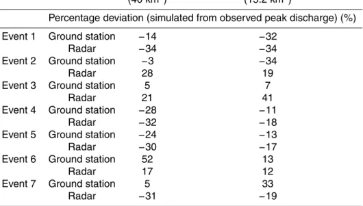
Print Version Interactive Discussion Table 6. Continued.

Rain input Brugga St. Wilhelmer Talbach

(40 km2) (15.2 km2)

Percentage deviation (simulated from observed peak discharge) (%)

Event 1 Ground station −14 −32

Radar −34 −34

Event 2 Ground station −3 −34

Radar 28 19

Event 3 Ground station 5 7

Radar 21 41

Event 4 Ground station −28 −11

Radar −32 −18

Event 5 Ground station −24 −13

Radar −30 −17

Event 6 Ground station 52 13

Radar 17 12

Event 7 Ground station 5 33

HESSD

Full Screen / Esc

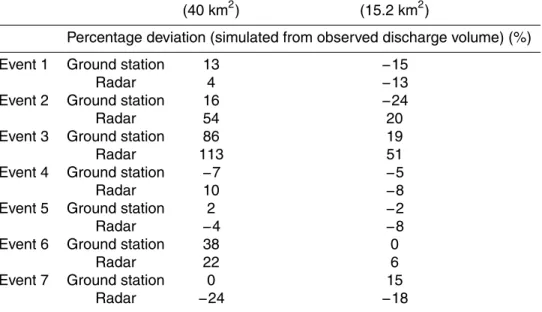
Print Version Interactive Discussion Table 6. Continued.

Rain input Brugga St. Wilhelmer Talbach

(40 km2) (15.2 km2)

Percentage deviation (simulated from observed discharge volume) (%)

Event 1 Ground station 13 −15

Radar 4 −13

Event 2 Ground station 16 −24

Radar 54 20

Event 3 Ground station 86 19

Radar 113 51

Event 4 Ground station −7 −5

Radar 10 −8

Event 5 Ground station 2 −2

Radar −4 −8

Event 6 Ground station 38 0

Radar 22 6

Event 7 Ground station 0 15

HESSD

Full Screen / Esc

Print Version Interactive Discussion

EGU

Figure 1

Fig. 1. The investigated catchments Brugga and St. Wilhelmer Talbach and its instrumentation

network.

HESSD

Full Screen / Esc

Print Version Interactive Discussion

EGU

Figure 2

Fig. 2. Simplified spatial distribution of dominant runoff generation areas: 1=Base flow,

2=In-terflow (delayed runoff), 3=surface and near surface runoff (fast runoff).

HESSD

Full Screen / Esc

Print Version Interactive Discussion

EGU

Figure 3

Fig. 3. Radar data calibration using the minimum square distance method for the cumulative

curves of both rainfall data sets.

HESSD

Full Screen / Esc

Print Version Interactive Discussion EGU 36 Figure 4a Figure 4b

Fig. 4. Spatial distribution of basin precipitation during the events 6 and 7.

HESSD

Full Screen / Esc

Print Version Interactive Discussion EGU Figure 5 03/06/02 05/06/02 07/06/02 09/06/02 11/06/02 disc har ge [ m ³/ s] 0 2 4 6 8 Q-observed Q-sim. ground station Q-sim. radar

Brugga catchment (40 km²)

Event 6

Event 7

Fig. 5. Hydrographs of the events 6 and 7 for the Brugga catchment (40 km2).

HESSD

Full Screen / Esc

Print Version Interactive Discussion EGU Figure 6 03/06/02 05/06/02 07/06/02 09/06/02 11/06/02 discharge [m³/ s] 0 2 4 6 8 Q-observed Q-sim. ground station Q-sim. radar

St. Wilhelmer TB catchment (15.2 km²)

Event 6

Event 7

Fig. 6. Hydrographs of the events 6 and 7 for the St. Wilhelmer Talbach catchment (15.2 km2).