A binary engine fuelling HD87643' s complex circumstellar environment, using AMBER/VLTI

(1)

HAL Id: hal-00408751

https://hal.archives-ouvertes.fr/hal-00408751v2

Submitted on 22 Sep 2009

HAL is a multi-disciplinary open access

archive for the deposit and dissemination of

sci-entific research documents, whether they are

pub-lished or not. The documents may come from

teaching and research institutions in France or

abroad, or from public or private research centers.

L’archive ouverte pluridisciplinaire HAL, est

destinée au dépôt et à la diffusion de documents

scientifiques de niveau recherche, publiés ou non,

émanant des établissements d’enseignement et de

recherche français ou étrangers, des laboratoires

publics ou privés.

A binary engine fuelling HD87643’ s complex

circumstellar environment, using AMBER/VLTI

Florentin Millour, Olivier Chesneau, Marcelo Borges Fernandes, Anthony

Meilland, Gilbert Mars, C. Benoist, Éric Thiébaut, Philippe Stee, K.-H.

Hofmann, Fabien Baron, et al.

To cite this version:

Florentin Millour, Olivier Chesneau, Marcelo Borges Fernandes, Anthony Meilland, Gilbert Mars, et

al.. A binary engine fuelling HD87643’ s complex circumstellar environment, using AMBER/VLTI.

Astronomy and Astrophysics - A&A, EDP Sciences, 2009. �hal-00408751v2�

(2)

September 22, 2009

A binary engine fuelling HD 87643’s complex circumstellar

environment

⋆

determined using AMBER/VLTI imaging

F. Millour

1

, O. Chesneau

2

, M. Borges Fernandes

2

, A. Meilland

1

,

G. Mars

3

, C. Benoist

3

, E. Thi´ebaut

4

, P. Stee

2

, K.-H. Hofmann

1

, F. Baron

5

, J. Young

5

,

P. Bendjoya

2

, A. Carciofi

6

, A. Domiciano de Souza

2

, T. Driebe

1

, S. Jankov

2

, P. Kervella

7

, R. G. Petrov

2

,

S. Robbe-Dubois

2

, F. Vakili

2

, L.B.F.M. Waters

8

, and G. Weigelt

1

1 _{Max-Planck Institut f¨ur Radioastronomie, Auf dem H¨ugel 69, 53121, Bonn, Germany,}

2 _{UMR 6525 H. Fizeau, Univ. Nice Sophia Antipolis, CNRS, Observatoire de la Côte d’Azur, F-06108 Nice cedex 2, France} 3 _{UMR 6202 Cassiopée, Univ. Nice Sophia Antipolis, CNRS, Observatoire de la Côte d’Azur, BP 4229, F-06304 Nice, France} 4 _{UMR 5574 CRAL, Univ. Lyon 1, Obs. Lyon, CNRS, 9 avenue Charles André, 69561 Saint Genis Laval cedex, France} 5 _{Astrophysics Group, Cavendish Laboratory, University of Cambridge, J.J. Thomson Avenue, Cambridge CB3 0HE, UK}

6 _{Instituto de Astronomia, Geof´ısica e Ciências Atmosféricas, Universidade de São Paulo, Rua do Matão 1226, Cidade Universitária,}

05508-900, S˜ao Paulo, SP, Brazil

7 _{LESIA, Observatoire de Paris, CNRS UMR 8109, UPMC, Univ. Paris Diderot, 5 place Jules Janssen, 92195 Meudon Cedex, France} 8 _{Faculty of Science, Astronomical Institute ‘Anton Pannekoek’, Kruislaan 403, 1098 SJ Amsterdam, The Netherlands}

Preprint online version: September 22, 2009

ABSTRACT

Context. The star HD 87643, exhibiting the “B[e] phenomenon”, has one of the most extreme infrared excesses for this object class.

It harbours a large amount of both hot and cold dust, and is surrounded by an extended reflection nebula.

Aims. One of our major goals was to investigate the presence of a companion in HD87643. In addition, the presence of close dusty

material was tested through a combination of multi-wavelength high spatial resolution observations.

Methods. We observed HD 87643 with high spatial resolution techniques, using the near-IR AMBER/VLTI interferometer with

baselines ranging from 60 m to 130 m and the mid-IR MIDI/VLTI interferometer with baselines ranging from 25 m to 65 m. These observations are complemented by NACO/VLT adaptive-optics-corrected images in the K and L-bands, and ESO-2.2m optical Wide-Field Imager large-scale images in the B, V and R-bands,

Results. We report the direct detection of a companion to HD 87643 by means of image synthesis using the AMBER/VLTI

instru-ment. The presence of the companion is confirmed by the MIDI and NACO data, although with a lower confidence. The companion is separated by ∼ 34 mas with a roughly north-south orientation. The period must be large (several tens of years) and hence the orbital parameters are not determined yet. Binarity with high eccentricity might be the key to interpreting the extreme characteristics of this system, namely a dusty circumstellar envelope around the primary, a compact dust nebulosity around the binary system and a complex extended nebula suggesting past violent ejections.

Key words. Techniques: high angular resolution – Techniques: interferometric – Stars: emission-line, Be – Stars: mass-loss – Stars: individual (HD 87643) – Stars: circumstellar matter

Introduction

Stars with the “B[e] phenomenon” are B-type stars with strong Balmer emission lines, numerous permitted Fe ii lines, and for-bidden O i and Fe ii lines in their optical spectrum. In addition, these stars exhibit a strong near and mid-IR excess due to cir-cumstellar dust (Allen & Swings 1976; Conti 1997). For brevity, we henceforth refer to stars showing the B[e] phenomenon as “B[e] stars”. The class of B[e] stars is composed of several sub-classes, including objects at different evolutionary stages and of

Send offprint requests to: F. Millour

e-mail: FMillour@mpifr-bonn.mpg.de

⋆ _{Based on observations made with the ESO Very Large Telescope at}

Paranal Observatory under programs 0575, 077.D-0095, 076.D-0141, 380.D-0340, and 280.C-5071, with the ESO 1.52-m and archival ESO data.

low, medium, and high mass (Lamers et al. 1998). Distances to-ward them are usually poorly known. As a consequence, the de-termination of the evolutionary state of B[e] stars is often uncer-tain.

Observations suggest that the wind of some of the most mas-sive B[e] stars (the so-called supergiant B[e] stars or sgB[e] in Lamers et al. 1998) is composed of two distinct components, as proposed by Zickgraf et al. (1985). The first component is a wind of low density in the polar regions; the second component is a wind of high density and low velocity located in the equato-rial region of the star. The thermal infrared excess is supposed to be produced in the outer parts of the equatorial wind where the temperature allows the formation of dust grains, but dust might also survive much closer to the star in a dense and compact disc. The formation of dusty environments around B[e] evolved objects is a challenge, with many theoretical issues (see

(3)

Kraus & Lamers 2003). A non-spherical, disc-like environment may be the key to understanding dust formation in sgB[e] stars. It could be attributed to the rapid rotation of these stars (e.g. Lamers & Pauldrach 1991; Bjorkman & Cassinelli 1993; Kraus 2006; Zsarg ´o et al. 2008) but could also be caused by compan-ions, since some B[e] stars were found to be binaries. Indeed, the number of companions detected around these objects is steadily growing (Miroshnichenko et al. 2004, 2006), but claims that all B[e] stars are binaries are still controversial (Zickgraf 2003).

The number of B[e] stars is rather limited, and many of them are unclassified (cited as unclB[e] in Lamers et al. 1998) be-cause they exhibit properties usually associated with young and evolved objects simultaneously.

Our group has undertaken a large observing campaign to investigate these poorly studied objects (sgB[e] and un-clB[e]) mostly using optical interferometry with the Very Large Telescope Interferometer (hereafter VLTI, see Stee et al. 2005, for an introduction to interferometric observations of Be and B[e] stars). Early results were published on the sgB[e] star CPD-57 2874 (Domiciano de Souza et al. 2007).

HD 87643 (Hen 3-365, MWC 198, IRAS 10028-5825) ap-pears to be a special case among sgB[e] and unclB[e] stars. It is a B2[e] star (Oudmaijer et al. 1998) that exhibits the largest infrared excess among this class and appears to be embedded in a complex nebula whose properties are reminiscent of the nebulae around LBVs (van den Bergh 1972; Surdej et al. 1981; Surdej & Swings 1983). HD 87643 is considered a unclB[e] by Lamers et al. (1998): it was classified as sgB[e] (see the esti-mation of the bolometric luminosity in McGregor et al. 1988; Cidale et al. 2001), under the assumption that it lies close to the Carina arm (2-2.5 kpc Oudmaijer et al. 1998; Miroshnichenko 1998; McGregor et al. 1988), but one can also find it classified as a Herbig star (Valenti et al. 2000; Baines et al. 2006). The v sin i of the central star is unknown since no pure photospheric line is detected in the visible spectrum. Clues to the disc-like geometry of the environment are provided by the polarisation ellipse in the U-Q plane across Hα (Oudmaijer et al. 1998). The detected PA is about 15◦_-20◦ _{(Yudin & Evans 1998; Oudmaijer et al. 1998).}

On the other hand, Baines et al. (2006) claimed to have de-tected an asymmetric outflow around HD87643 using spectro-astrometry. However, they also note that “HD 87643 stands out in the complexity of its spectro-astrometry”, compared with the numerous other Herbig Be stars they observed.

HD 87643 has displayed a long-term decline of the vi-sual brightness for the last 30 yrs, from V ≈ 8.5/8.8 in 1980 (Miroshnichenko 1998), to V ≈ 9.3/9.4 in early 2009 (Pojma´nski 2009). This decline is superimposed on shorter-term variations, such as a 0.5 mag decrease in ≈1 month, followed by a 0.7 mag increase in ≈5 months, seen in the ASAS photometric survey (Pojma´nski 2009) between JD 2453000 and JD 2453180. Yudin & Evans (1998) also noted that HD87643 shows Algol-like variability, the star showing variations “on a timescale of days”, and being “bluer during brightness minima”.

The totality of the ISO/SWS 2-45 µm mid-IR emission from HD 87643 seems concentrated within the smallest ISO aperture (14” x 22”), and at 10 µm, the dusty environment is unresolved on a 1” scale (Voors 1999). The ISO/LWS spectrum also contin-ues from the shorter-wavelength SED without any jump, which is an additional sign that the mid-IR emission is compact. The disc-like geometry is strongly supported by the huge infrared excess exhibited by the source, the large absorption of the cen-tral star flux, and the polarimetric data. Voors (1999) proposed that the disc might be a circumbinary disc.

In this paper we report new observations that bring a new in-sight into this interesting object, proving the presence of a com-panion, a resolved circum-primary dust envelope (most likely a disc), and circumbinary material.

The outline of the article is as follows: the observations and data recorded are presented in Sect. 1, then we present and dis-cuss the main results from our observing campaign in Sect. 2, and give a global view of the system, considering this new infor-mation, in Sect. 3.

1. Observations and data processing

1.1. AMBER/VLTI near-IR interferometry

HD 87643 was observed at the ESO/Paranal observatory with the Astronomical Multi BEam Recombiner (AMBER), the near-infrared instrument of the VLTI (Petrov et al. 2007). The obser-vations were carried out on February 18, 2006 in medium spec-tral resolution (R = 1500) and during a series of nights in March 2008 at low spectral resolution (R = 35). AMBER uses three 8m telescopes (Unit Telescopes, hereafter UT) or three 1.8m telescopes (Auxiliary Telescopes, hereafter AT). The calibration stars used were HD 109787, HD 86440, HD 101531, HD 63744 and ǫ Oph. Details of the observations can be found in Table 1.

Table 1. AMBER and MIDI observing logs.

projected baseline

Date Stations Length PA

[meter] [degrees] AMBER 1 (UT) 18/02/2006, 3h UT1-3-4 95, 57, 129 22, 88, 46 18/02/2006, 8h UT1-3-4 71, 62, 102 65, 145, 102 AMBER 2 (AT) 01/03/2008, 2h K0-G1-A0 83, 78, 128 -168, -94, -132 05/03/2008, 3h G1-D0-H0 63, 64, 60.0 -59, 64, 3 06/03/2008, 5h G1-D0-H0 69, 60, 58 -37, 90, 19 06/03/2008, 7h G1-D0-H0 71, 52, 33 -15, 117, 33 10/03/2008, 3h H0-G0-E0 31, 15.6, 46.8 -102 11/03/2008, 0h H0-G0-E0 32, 16, 47 -147 12/03/2008, 0h H0-G0-E0 32, 16, 48 -145 MIDI (AT) 26/02/2006, 4h D0-G0 31.3 76.3 27/02/2006, 6h A0-G0 57.1 101.3 01/03/2006, 1h A0-G0 63.5 38.1 01/03/2006, 5h A0-G0 61.1 85.1 19/04/2006, 4h D0-G0 25.4 123.1 23/05/2006, 2h A0-G0 51.7 120.0 25/05/2006, 1h A0-G0 54.4 110.6

The data were processed with the standard AMBER data reduction software (amdlib 2.1, see for instance Tatulli et al. 2007; Millour et al. 2004) plus a series of advanced scripts to calibrate the data (Millour et al. 2008). The AMBER DRS per-forms a fringe fitting instead of Fourier transper-forms and computes interferometric data products such as V2_{and closure phases (for} a review of the interferometric data analysis, see: Haniff 2006; Monnier 2006; Millour 2008). We performed the reduction us-ing standard selection criteria (see for instance appendix C in Millour et al. 2007) for the individual exposures, rejecting 80% of the data before averaging the data products. The additional scripts allowed us to compute realistic error bars, including the uncertainties on the diameters of the calibration stars, the instru-ment atmosphere transfer function instabilities, and the

(4)

funda-mental noise. The study of the transfer function provided by dif-ferent calibrators gives an estimate of absolute errors on V2 be-tween 0.05 and 0.1. The visibilities and closure phases are shown in Fig. 3.

1.2. MIDI/VLTI mid-IR interferometry

The observations of HD 87643 at the ESO/Paranal obser-vatory using the MID-Infrared instrument (hereafter MIDI, Leinert et al. 2003, 2004) were carried out from February un-til May 2006. MIDI is the mid-infrared (N-band, 7.5-13.5 µm) two-telescope combiner of the VLTI, operating like a classical Michelson interferometer. In our case, only the ATs were used since HD 87643 is bright in the mid-IR (156 Jy). We used a stan-dard MIDI observing sequence, as described by Ratzka et al. (2007). The source was observed in the so-called High-Sens mode, implying that the photometry from each individual tele-scope is performed subsequently to the recording of the fringes. The low spectral resolution (R=30) provided by the prism was used. The data consist of 7 visibility spectra and one flux spec-trum (PSF 1.2” with ATs). The errors on the visibilities, includ-ing the internal ones and those from the calibrator diameter un-certainty, range from 0.05 to 0.15. The MIDI spectrum was diffi-cult to calibrate, and the accuracy of the absolute photometry is not better than 30%, although one can see in Fig. 4 that the MIDI spectrum agrees well with the IRAS (Olnon et al. 1986) and the ISO spectra (affected by problems of ’gluing’ between different spectral bands, as reported in Voors 1999). The log of the ob-servations is given in Table 1. We used two different MIDI data reduction packages: MIA developed at the Max-Planck-Institut f¨ur Astronomie and EWS developed at the Leiden Observatory (MIA+EWS1, ver.1.5.1). The resulting visibilities can be seen in Fig. 4.

1.3. NACO/VLT adaptive optics assisted imaging

We observed HD 87643 at the ESO/Paranal observatory with the NACO adaptive optics camera (NAos adaptive optics sys-tem combined with the COnica camera, Rousset et al. 2003) at-tached to UT4 of the Very Large Telescope (VLT). NACO was operated in the visual wavefront sensor configuration. We ob-served the target with Ks (2.2µm) and L′ _{(3.8µm) broad-band}

filters. The star HD 296986 was used to derive the point-spread function (PSF). The S13 camera mode was used for Ks, with a 13 mas per pixel scale and a 14”×14” field of view. In L′, using camera mode L27, the field of view was 28”×28” and the pixel scale was 27.1 mas. The auto-jitter mode was used, which, at each exposure, moves the telescope in a random pattern within a box of side 7” in Ks and 15” in L′_{. The journal of observations}

can be found in Table 2.

The data reduction was performed using our own scripts. First, bad pixels were removed (i.e. interpolated using the ad-jacent pixel values) and a flat-field correction was applied to the data. Then, the sky was computed as the median of all expo-sures and subtracted exposure by exposure. A visual inspection of each exposure allowed us to check the PSF quality. The “bad” ones were removed for the next step. This allowed us to signifi-cantly improve the final data product image quality compared to the standard pipeline-reduced frames. This also led us to disre-gard the 20/03/2008 data-sets, which were in any case flagged as “failed” in the observing log. A cross-correlation technique was

1 _{Available at}

http://www.strw.leidenuniv.nl/∼_nevec/MIDI

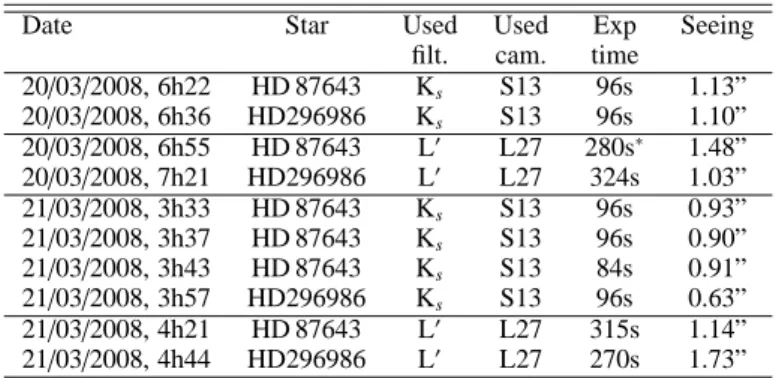
Table 2. Journal of observations with NACO/VLT. All stars

were observed with a neutral density filter.

Date Star Used Used Exp Seeing

filt. cam. time

20/03/2008, 6h22 HD 87643 Ks S13 96s 1.13” 20/03/2008, 6h36 HD296986 Ks S13 96s 1.10” 20/03/2008, 6h55 HD 87643 L′ _L27 _280s∗ _1.48” 20/03/2008, 7h21 HD296986 L′ _L27 _324s _1.03” 21/03/2008, 3h33 HD 87643 Ks S13 96s 0.93” 21/03/2008, 3h37 HD 87643 Ks S13 96s 0.90” 21/03/2008, 3h43 HD 87643 Ks S13 84s 0.91” 21/03/2008, 3h57 HD296986 Ks S13 96s 0.63” 21/03/2008, 4h21 HD 87643 L′ _L27 _315s _1.14” 21/03/2008, 4h44 HD296986 L′ _L27 _270s _1.73” ∗ saturated

then used to re-centre the images with about 1 pixel accuracy. Finally, all the selected frames were co-added, resulting in the total exposure time shown in Table 2.

As a result, we got a pair of science star/PSF star images for each observation (which were repeated due to changing weather conditions and saturation of the detector). The PSF FWHM is 75±4 mas in the Ks-band and 111±6 mas in the L’-band. In addi-tion to a deconvoluaddi-tion attempt presented in Sect. 2.2, we com-puted radial profiles to increase the dynamic range from about ≈103_{per pixel to ≈ 10}4_-105_{. The result can be found in Fig. 5.}

1.4. 2.2m/WFI large-field imaging

We retrieved unpublished archival ESO/Wide-Field Imager (WFI) observations of the nebula around HD 87643 from the ESO database2_{carried out on March 15 and 16, 2001. The WFI} is a mosaic camera attached to the ESO 2.2m telescope at the La Silla observatory. It consists of eight 2k×4k CCDs, forming an 8k×8k array with a pixel scale of 0.238” per pixel. Hence, a single WFI pointing covers a sky area of about 30’×30’. The observations were performed in the B, V, Rc and Icbroadband filters and in the narrow-band filter in the Hα line (λ = 658nm, FWHM = 7.4nm). However, we used only the observations with B, V, and R filters given that it is a reflection nebula only (Surdej et al. 1981). In order to cover the gaps between the WFI CCDs and to correct for moving objects and cosmic ray hits, for each pointing, a sequence of five offset exposures was performed in each filter.

The data reduction was performed using the package alambic developed by B. Vandame based on tools available from the multi-resolution visual model package (MVM) by Ru´e & Bijaoui (1997). The image is shown in Fig. 6.

2. New facts about HD 87643

2.1. Interferometry data: A binary star plus a compact dusty disc

From the sparse 2006 AMBER medium spectral resolution data, the structure of the source could not be inferred unambiguously. The squared visibilities from 2006 did not show any significant variation with spatial frequency. The closure phases were mea-sured as zero within the error estimates (see Fig. 3).

(5)

The Brγ emission line appears clearly in the AMBER calibrated spectrum after using the technique described in Hanson et al. (1996) of fitting and removing the Brγ line for the calibrator. The resulting Brγ line accounts for 15% of the con-tinuum flux at its maximum and is spread over 5 spectral pixels (250 km · s−1_{), similar to what is reported in McGregor et al.} (1988). −200 0 200 −200 0 200 E <−−−−−−−− sp. freq. (cycles/as) sp. freq. (cycles/as) −−−−−−−−> N −200 0 200 −200 0 200 E <−−−−−−−− sp. freq. (cycles/as) sp. freq. (cycles/as) −−−−−−−−> N

Fig. 1. UV coverage obtained on HD87643 in the H-band (left),

in the K-band (right). The radial lines are caused by the different wavelengths within the bands.

The extensive AMBER low spectral resolution data, secured in 2008 (see Fig. 3), show large variations of V2 and closure phases and clearly indicate a modulation from a binary source. Given the good uv coverage (see Fig. 1) and the quality of the data, we undertook an image reconstruction process, aiming to determine the best models to use for the interpretation.

2.1.1. Image reconstruction

The images in Fig. 2 were reconstructed from the AMBER squared visibilities and closure phases using the MIRA software (Thi´ebaut 2008). MIRA compares the visibilities and the clo-sure phases from a modelled image with the observed data using a cost-estimate optimisation, including a priori information such as image positivity (all image pixels are positive) and compact-ness of the source (using a so-called L2-L1 regularisation, see Thi´ebaut 2008, for details).

Separate image reconstructions were made using the H-band and K-band data, assuming that the object was achromatic over the whole band considered. MIRA needs a starting image, but we found that the image reconstruction result did not significantly depend on it. Extensive tests and comparisons with other soft-ware (Hofmann & Weigelt 1993; Baron & Young 2008, see ap-pendix A) made us confident that we could distinguish between artifacts and real structures in the images. The theoretical field of view, computed using the formula 2.44λ/Bmin, is ≈ 70 mas,

Bminbeing the shortest projected baseline (15 m). We convolved the K-band image with a Gaussian beam of FWHM λ/Bmax = 3.5 mas and the H-band one with a beam of λ/Bmax = 2.7 mas,

Bmax being the longest projected baseline (128 m). The image noise is of the order of 1%.

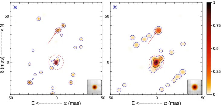
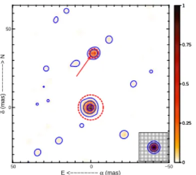
The reconstructed image reveals the presence of a com-panion star with a plane-of-sky separation of ≈34.5 mas (see Table 3). the K-band image also reveals an extended structure detected around the main star. We cannot assess any elonga-tion of this resolved structure due to the poor UV coverage in the NW direction. We emphasise that there is still a 180◦

un-certainty due to the overall unun-certainty on the AMBER closure phase sign (and not due to the image reconstruction process: see appendix A.1.3). We will refer in the following to “the northern” and “the southern” components.

We also extracted relative fluxes for the different components within the dashed circles in Fig. 2 (see Table 3), but one has to bear in mind that extracting such fluxes is affected not only by large errors, but also potentially by large systematics. Therefore, we also performed the flux measurements using model-fitting.

2.1.2. Model fitting

In Section 2.1.1., we show that the 2008 AMBER data can be di-rectly interpreted assuming the presence of a binary source with a plane-of-sky separation of ≈34 mas and a P.A. of ≈ 0◦ _(see

Table 3) and a resolved southern component. We fitted the data using such a model to obtain more accurate component fluxes. The images show a series of large-scale artifacts (i.e. flux whose spatial location is poorly constrained), accounting for a large fraction of the total integrated flux. These artifacts are related to the lack of data with high visibilities at small spatial frequen-cies. We therefore also included an extended component to our model, fully resolved on all AMBER baselines.

Our model-fitting used the scientific software yorick3 com-bined with the AMBER data reduction software amdlib. This tool was complemented with a series of optimisation scripts de-veloped by the JMMC (B´echet et al. 2005) and others dede-veloped by us. We judge that the resulting fits were satisfactory, even though the formal χ2is about 40 (see Fig. 3), probably due to an underestimation of the errors during the data reduction.

0 10 20

0.1 0.2 0.3

Sp. Freq (Bproj/λ, cycles/arcsec)

S q u ar ed v is ib il it y S q u ar ed v is ib il it y S q u ar ed v is ib il it y S q u ar ed v is ib il it y S q u ar ed v is ib il it y S q u ar ed v is ib il it y S q u ar ed v is ib il it y S q u ar ed v is ib il it y S q u ar ed v is ib il it y S q u ar ed v is ib il it y S q u ar ed v is ib il it y S q u ar ed v is ib il it y S q u ar ed v is ib il it y S q u ar ed v is ib il it y

Fig. 4. MIDI visibilities (in Gray with error bars), projected on the direction of the detected binary star and compared with our model (in thick black line).

The MIDI data show complex, spectrally dependent visi-bility variations from one observation to another (see Fig. 4). Spherical and even 2-D axi-symmetric dusty models were not able to account for this data set. We used the separation and P.A. inferred from the AMBER 2008 data as initial values for the fit-ting of the AMBER 2006 and MIDI 2006 measurements.

The result of such a fit shows that our binary model is compatible with both the AMBER and MIDI 2006 data sets. Moreover, we find that the MIDI separation is close to that derived from the AMBER 2008 data set. The P.A. of the secondary component differs slightly between near- and mid-infrared, which might be due to an offset of the dust structure

3 _{open-source scientific software freely available at the following}

(6)

(a) −50 0 50 0 50 (b) −50 0 50 0 50 0 0.25 0.5 0.75 1 0 0.25 0.5 0.75 1

E <−−−−−−−−

α

(mas)

E <−−−−−−−−

α

(mas)

δ

(mas) −−−−−−−−> N

Fig. 2. Aperture-synthesis images of HD87643 reconstructed from the H-band AMBER data (panel 2a) and the K-band data (panel 2b), assuming the source is achromatic in each band. Contours with 50, 10, and 1% of the maximum flux are shown, and the beam size is shown in the lower-right box. The arrow shows the companion star, whereas the dashed circles show the trusted structures in the images.

0 50 100 150

0.2 0.4

S q u ar ed v is ib il it y S q u ar ed v is ib il it y S q u ar ed v is ib il it y S q u ar ed v is ib il it y S q u ar ed v is ib il it y S q u ar ed v is ib il it y S q u ar ed v is ib il it y S q u ar ed v is ib il it y S q u ar ed v is ib il it y S q u ar ed v is ib il it y S q u ar ed v is ib il it y S q u ar ed v is ib il it y 0 50 100 150 −10 −5 0 5 10

Sp. Freq largest base (Bproj/λ, cycles/arcsec)

Closure phase (rad)

0 50 100 150 200

0.2 0.4 0.6

Sp. Freq (BSp. Freq (BSp. Freq (BSp. Freq (BSp. Freq (BSp. Freq (BSp. Freq (BSp. Freq (BSp. Freq (BSp. Freq (BSp. Freq (BSp. Freq (BSp. Freq (BSp. Freq (BSp. Freq (BSp. Freq (BSp. Freq (BSp. Freq (BSp. Freq (BSp. Freq (BSp. Freq (BSp. Freq (BSp. Freq (BSp. Freq (BSp. Freq (BSp. Freq (BSp. Freq (BSp. Freq (BSp. Freq (BSp. Freq (BSp. Freq (BSp. Freq (BSp. Freq (BSp. Freq (BSp. Freq (BSp. Freq (BSp. Freq (BSp. Freq (BSp. Freq (BSp. Freq (BSp. Freq (BSp. Freq (BSp. Freq (BSp. Freq (BSp. Freq (BSp. Freq (BSp. Freq (BSp. Freq (BSp. Freq (BSp. Freq (BSp. Freq (BSp. Freq (BSp. Freq (BSp. Freq (BSp. Freq (BSp. Freq (BSp. Freq (BSp. Freq (BSp. Freq (BSp. Freq (BSp. Freq (BSp. Freq (Bprojprojprojprojprojprojprojprojprojprojprojprojprojprojprojprojprojprojprojprojprojprojprojprojprojprojprojprojprojprojprojprojprojprojprojprojprojprojprojprojprojprojprojprojprojprojprojprojprojprojprojprojprojprojprojprojprojprojprojprojprojproj/λ, cycles/arcsec)/λ, cycles/arcsec)/λ, cycles/arcsec)/λ, cycles/arcsec)/λ, cycles/arcsec)/λ, cycles/arcsec)/λ, cycles/arcsec)/λ, cycles/arcsec)/λ, cycles/arcsec)/λ, cycles/arcsec)/λ, cycles/arcsec)/λ, cycles/arcsec)/λ, cycles/arcsec)/λ, cycles/arcsec)/λ, cycles/arcsec)/λ, cycles/arcsec)/λ, cycles/arcsec)/λ, cycles/arcsec)/λ, cycles/arcsec)/λ, cycles/arcsec)/λ, cycles/arcsec)/λ, cycles/arcsec)/λ, cycles/arcsec)/λ, cycles/arcsec)/λ, cycles/arcsec)/λ, cycles/arcsec)/λ, cycles/arcsec)/λ, cycles/arcsec)/λ, cycles/arcsec)/λ, cycles/arcsec)/λ, cycles/arcsec)/λ, cycles/arcsec)/λ, cycles/arcsec)/λ, cycles/arcsec)/λ, cycles/arcsec)/λ, cycles/arcsec)/λ, cycles/arcsec)/λ, cycles/arcsec)/λ, cycles/arcsec)/λ, cycles/arcsec)/λ, cycles/arcsec)/λ, cycles/arcsec)/λ, cycles/arcsec)/λ, cycles/arcsec)/λ, cycles/arcsec)/λ, cycles/arcsec)/λ, cycles/arcsec)/λ, cycles/arcsec)/λ, cycles/arcsec)/λ, cycles/arcsec)/λ, cycles/arcsec)/λ, cycles/arcsec)/λ, cycles/arcsec)/λ, cycles/arcsec)/λ, cycles/arcsec)/λ, cycles/arcsec)/λ, cycles/arcsec)/λ, cycles/arcsec)/λ, cycles/arcsec)/λ, cycles/arcsec)/λ, cycles/arcsec)/λ, cycles/arcsec)

S q u ar ed v is ib il it y S q u ar ed v is ib il it y S q u ar ed v is ib il it y S q u ar ed v is ib il it y S q u ar ed v is ib il it y S q u ar ed v is ib il it y S q u ar ed v is ib il it y S q u ar ed v is ib il it y S q u ar ed v is ib il it y S q u ar ed v is ib il it y S q u ar ed v is ib il it y S q u ar ed v is ib il it y S q u ar ed v is ib il it y S q u ar ed v is ib il it y S q u ar ed v is ib il it y S q u ar ed v is ib il it y S q u ar ed v is ib il it y S q u ar ed v is ib il it y S q u ar ed v is ib il it y S q u ar ed v is ib il it y S q u ar ed v is ib il it y S q u ar ed v is ib il it y S q u ar ed v is ib il it y S q u ar ed v is ib il it y S q u ar ed v is ib il it y S q u ar ed v is ib il it y S q u ar ed v is ib il it y S q u ar ed v is ib il it y S q u ar ed v is ib il it y S q u ar ed v is ib il it y S q u ar ed v is ib il it y S q u ar ed v is ib il it y S q u ar ed v is ib il it y S q u ar ed v is ib il it y S q u ar ed v is ib il it y S q u ar ed v is ib il it y S q u ar ed v is ib il it y S q u ar ed v is ib il it y S q u ar ed v is ib il it y S q u ar ed v is ib il it y S q u ar ed v is ib il it y S q u ar ed v is ib il it y S q u ar ed v is ib il it y S q u ar ed v is ib il it y S q u ar ed v is ib il it y S q u ar ed v is ib il it y S q u ar ed v is ib il it y S q u ar ed v is ib il it y S q u ar ed v is ib il it y S q u ar ed v is ib il it y S q u ar ed v is ib il it y S q u ar ed v is ib il it y S q u ar ed v is ib il it y S q u ar ed v is ib il it y S q u ar ed v is ib il it y S q u ar ed v is ib il it y S q u ar ed v is ib il it y S q u ar ed v is ib il it y S q u ar ed v is ib il it y S q u ar ed v is ib il it y S q u ar ed v is ib il it y S q u ar ed v is ib il it y S q u ar ed v is ib il it y S q u ar ed v is ib il it y S q u ar ed v is ib il it y S q u ar ed v is ib il it y S q u ar ed v is ib il it y S q u ar ed v is ib il it y S q u ar ed v is ib il it y S q u ar ed v is ib il it y S q u ar ed v is ib il it y S q u ar ed v is ib il it y S q u ar ed v is ib il it y S q u ar ed v is ib il it y S q u ar ed v is ib il it y S q u ar ed v is ib il it y S q u ar ed v is ib il it y S q u ar ed v is ib il it y S q u ar ed v is ib il it y S q u ar ed v is ib il it y S q u ar ed v is ib il it y S q u ar ed v is ib il it y S q u ar ed v is ib il it y S q u ar ed v is ib il it y 0 50 100 150 200 −2 0 2

Closure phase (rad)

Fig. 3. Squared visibilities (left) and closure phases (right) plotted as a function of spatial frequency, projected onto the inferred binary position angle. The 2006 AMBER data set is seen on top, 2008 on the bottom. The model involving a binary system composed of one resolved and one unresolved component plus a fully resolved background is shown with a solid black line.

compared to the main star. The total flux seen by MIDI is dom-inated by a fully resolved background in addition to the unre-solved binary components (Table 3). The AMBER 2006 data set is too limited to provide a strong constraint on the the flux ratios; therefore, we do not use them in the following analysis.

We stress that the MIDI data is affected by an independent 180◦_{orientation ambiguity to the AMBER ambiguity (due to the}

uncalibrated closure phase sign), as it only consists of squared visibility data. Hence, we cannot definitely relate the compo-nent fluxes derived from the MIDI data to those derived from the AMBER data.

(7)

Table 3. Estimated diameter of the envelope, position of the secondary source, and respective fluxes, relative to the total flux.

The envelope flux includes both the southern component and its compact circumstellar envelope fluxes. The errors given for the model-fitting reflects only formal estimates from the χ2_value.

AMBER (model fitting) AMBER (Image reconstruction) MIDI (2006)

Wavelength ( µm) 1.55 2.45 H-band K-band 8.1 10.5 12.9

Point + Gaussian + Background Image Point + Gaussian + Background Envelope size (mas) 3.1 ± 0.1 4.5 ± 0.1 - - ≤6.5 ≤10.6 ≤3.5 Envelope flux (% total flux) 61 ± 2 72 ± 2 ≈46 ≈59 17 ± 2 9 ± 1 6.3 ± 0.5 Background flux (% total flux) 12 ± 2 9 ± 2 ≈44 ≈25 69 ± 13 77 ± 9 75 ± 9 Secondary flux (% total flux) 27 ± 1 19 ± 1 ≈10 ≈16 14 ± 3 15 ± 2 19 ± 2 Secondary separation (mas) 33.48 ± 0.03 34.5 ± 0.5 34.6 ± 0.5 36.8 ± 0.1 Secondary PA (◦

) −4.50 ± 0.03 −2.5 ± 0.8 −4.1 ± 0.8 −26.1 ± 1.7

2.2. NACO K-band imaging: a very compact dusty environment

We performed a deconvolution process on our NACO images. Using both speckle techniques and the Lucy-Richardson decon-volution algorithm, an elongated north-south compact structure could be detected in the K-band but not in the L-band. This is compatible with the AMBER data.

In addition, we tested the presence of dusty emission in the surroundings of the star by azimuthally integrating the flux to increase the dynamic range (see Fig. 5). In the K-band, no ex-tended emission is detectable up to 1.5 arc-seconds (at larger distances, ghost reflections or electronic ghosts impair the dy-namic range of the images) and a faint emission can be seen in the L-band from 0.5 to 3.0 arc-seconds. This might be linked to the fully resolved component seen in our AMBER data, and therefore probably implies that it is much more extended than the field of view of AMBER. However, the dynamic range of our images (≈ 103per pixel, and ≈ 104-105 for the radial pro-files) does not allow us to access the spatial distribution of such a dusty nebula.

2.3. WFI imaging: The large scale nebula revisited

The extended nebula was discovered and studied by van den Bergh (1972); Surdej et al. (1981); Surdej & Swings (1983). In particular, using the 3.6m ESO telescope at La Silla, Surdej & Swings (1983) showed that the structure was a reflection nebula with a 60-100” extension.

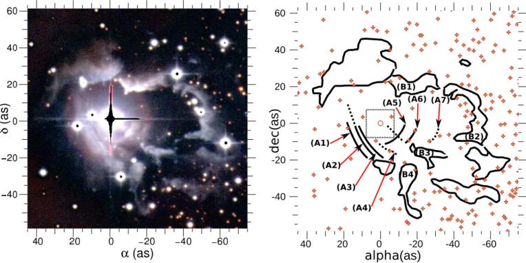
The nebula revealed by the WFI instrument (see Fig. 6) with the 2.2m telescope at La Silla shows increased dynamic range but shares the same spatial resolution and global morphology as the previous works. The nebular structures are primarily seen in the north-west quadrant from the central star in the form of an extended and structured filamentary feature at distances of 15-20” (north) to 35-50”(west). In some places, labelled (B1) to (B4), the nebula appears blown-up by the central star wind, with clumpy and patchy features.

This structure has no extended counterpart in the south-east region, where arc-like structures (labeled (A1) to (A4) in the fig-ure) can be seen closer to the star (at 10”, 12”, 14”, and 18” respectively). These arcs are spaced by two to four arc-secs and might come from past ejection events.

In the south-west region, at 12”, 19”, and 30” respectively from the star, two bright and one faint arc can be seen (labelled (A5) to (A7) in the figure). These arcs do not appear to be con-nected to the previously-mentioned ones.

A star count made using sextractor (Bertin & Arnouts 1996) gives values twice as low in the east half than in the west half of the image. No significant relative change in the counts as a

function of filter is detectable over the field. This indicates that there is a total absorption screen somewhere in the field, totally masking the background stars in the east half of the WFI image. We note that it corresponds to a dark cloud in the eastern part, clearly seen in our WFI image in front of red (hydrogen ?) neb-ular emission. However, we cannot directly assess if this screen is in front or behind HD 87643 and its nebula.

3. Discussion

3.1. Adopting a distance for the system

HD 87643 is thought to be an evolved B[e] star, and the neb-ula suggests a link to the LBV class (Surdej & Swings 1983). HD 87643 stands out as unusual compared to typical sgB[e] stars such as CPD-57 2874, since ISO SWS and LWS spectra show a considerable amount of cold dust (T≤150K).

McGregor et al. (1988) implicitly assumed that HD 87643 is a supergiant in order to determine its distance, based on its location in the direction of the Carina Arm. Such a location would place it at a distance of 2-3 kpc. However, the distance of HD 87643 has never been accurately measured. When other estimates of the distance are found in the literature, the values are usually much smaller. These were derived by:

1. van den Bergh (1972) and de Freitas Pacheco et al. (1982): 530 pc, based on Kurucz models for a B2V star (Teff = 18000 K, E(B-V) = 0.63 mag, R∗= 6 R⊙);

2. Surdej et al. (1981): 1 kpc, based on MV= -4.1 derived from photometry;

3. Shore et al. (1990): 1.2 kpc, using the IUE UV spectrum; 4. Lopes et al. (1992): 2-3 kpc using the equivalent width

(here-after, EW) of Nai lines. We note, however, that the high reported value of 2.9 kpc is affected by a factor of 2 error in their application of the statistical relation cited by Allen (1973). Considering the correct relation (r = 2.0D, r be-ing the distance in kpc and D bebe-ing the mean EW in Å of the two Na D lines), the distance would be 1.46 kpc (Lopes, private communication). The EW were measured using low-resolution spectra, implying a possible contamination of cir-cumstellar origin;

5. Oudmaijer et al. (1998): 1-6 kpc, also based on the Nai D-line equivalent widths derived from a higher-resolution spec-trum, but using data on the interstellar extinction for nearby stars instead of the relationship from Allen (1973). The large uncertainty of this distance is due to the large scatter of the extinction values in the Carina arm line of sight.

6. Zorec (1998): 1.45 kpc, based on a SED fitting using various assumptions.

(8)

Fig. 5. NACO radial profiles. Left is the Ksfilter and right is the L

′

filter. HD 87643 is shown as full lines (3 observations in Ks, and one in L’, see Table 2). The calibrator star is shown as a dotted line.

Fig. 6. Reflection nebula around HD 87643, as a composite of R, V and B filters (left), together with a sketch presenting the main structures (right). The saturated regions are masked by black zones in the image. This image is a small part of the 30’x30’ field-of-view of the WFI observations. The sketch shows HD 87643 as a red circle, whereas other stars are marked as red crosses. The nebular contours are drawn as black lines and the prominent features are labelled (A1) to (A7) for arc-like structures and (B1) to (B4) for apparently blown-up nebular structures. Structures which are faint or uncertain are marked as dotted lines.

Therefore, we arbitrarily use the distance of 1.5 kpc, as sug-gested by some of these works, in the subsequent parts of the present article.

3.2. Orbital characteristics of the binary system

One of the main results from the AMBER interferometric obser-vations is that HD 87643 is a double system. In the K-band, the NACO image core is also significantly resolved with an elonga-tion in the same direcelonga-tion as the AMBER binary. The separaelonga-tion and position angle of the components are well constrained by the data. It is more difficult to derive an accurate flux ratio, given the complexity of the object. Here, we shall summarise our results, from the most constrained ones to the most speculative.

– The plane-of-sky separation of the components is 34 ±

0.5 mas. At 1.5 kpc, it corresponds to a projected separa-tion of 51 ± 0.8 AU. As a comparison, the separasepara-tion of the interacting components of β Lyrae (Zhao et al. 2008) is of

the order of 0.2 AU (orbital period 12 d), the separation of the γ2Velorum (Millour et al. 2007) colliding-wind compo-nents is of the order of 1.3 AU (period 78 d), and the approxi-mate separation of the high-mass binary θ1_{Ori C (Stahl et al.} 2008; Patience et al. 2008; Kraus et al. 2007) is 15-20 AU (orbital period of between 20 and 30 yrs).

– Therefore, the orbital period of HD87643 is large,

approxi-mately 20-50 years. In particular, no significant orbital mo-tion is seen between our 2006 and 2008 data sets.

– The orbital plane might be seen at a high inclination (i.e.

close to edge-on). Indeed, this is suggested by the high level of observed polarisation (Oudmaijer et al. 1998). The large-scale measurements also seem to imply a bipolar morphology (see Sect. 3.3). In addition, HD87643 shows photometric variability. The short-term variations (e.g. am-plitude ∼0.5mag, seen in the ASAS light curves and in Miroshnichenko 1998) are similar to Algol-like variability (Yudin & Evans 1998) and are therefore probably a

(9)

conse-quence of the time-variable absorption by the material pass-ing through the line-of-sight. This is also in favour of a highly inclined (edge-on) disc-like structure.

– The orbit might be highly eccentric. This hypothesis is

sup-ported by the periodic structures seen in the large-scale neb-ula (see Sect. 3.3) that would suggest periodic eruptions. These eruptions would be a sign of close encounters of the binary components, while we observed a well-separated bi-nary.

3.3. A link to the larger-scale nebula

Dust is found at large distances east and west of the nebula, with fluxes reaching 15 Jy at 16.7 µm (ISO/CAM1, offset of 25” from the star, aperture 20”x14”), whereas no flux is detected in the north and south positions4. This points to a bipolar nebulosity in the east-west direction.

As mentioned by Surdej et al. (1981), the number of field stars decreases in the south-east direction. Also from this work (Sect. 2.3), the number of visible stars in the eastern part of the WFI image of the nebula is about 2 times less than in the western part. This may mean that the other side of a symmetrical bipolar nebula remains hidden in our WFI image.

Finally, we note that inferring the geometry of the nebula is potentially of great importance as this reflection nebula al-lows one to study the central star from different viewing angles, i.e probing different latitudes of the central star. The anisotropy of the star flux was already noted in Surdej et al. (1981) and Surdej & Swings (1983).

Oudmaijer et al. (1998) and Baines et al. (2006) measured expansion velocities of ≈ 1000 km · s−1_{. Therefore one can} es-timate an ejection time for the nebula: at 1.5 kpc distance and taking a 50” extent, one gets ≈355 yrs.

For the arc-like structures and the same value for the expan-sion speed and distance, we find the following values: ≈71 yrs for A1, ≈85 yrs for A2, ≈100 yrs for A3, and ≈128 yrs for A4. This first series gives ejection time intervals of ≈14, ≈14 and ≈28 yrs, respectively, between two consecutive arcs. This might be the trace of a periodic ejection with a period of ≈14 yrs on the assumption that one arc (between A3 and A4) is not seen in our image. However, this periodicity is probably affected by a projection effect since the v sin i of the arcs is not known and they appear to be almost linear (instead of circular); hence, the ≈14 yrs periodicity is a lower limit. Concerning the second series of arcs, we find ≈85 yrs for A5, ≈135 yrs for A6, and ≈213 yrs for A7. In this case, the apparent ejection time intervals between two consecutive arcs are ≈50 yrs and ≈78 yrs. Given that the arcs appear almost circular in the image, we can assume that the pro-jection angle is close to 90◦_{. Since we have only three arcs in}

this case (with one barely seen), we can only put an upper limit of ≈50 yrs on the periodicity of these ejections.

These broken structures suggest short, localised ejection that might coincide with short periastron passages of the compan-ion, triggering violent mass-transfer between the components. Therefore, we tentatively infer limits between 14 and 50 yrs for the periodicity of the binary system. Monitoring the system at high angular resolution over a timescale of a few dozen years would most likely bring an unprecedented insight into this sys-tem.

4 _{These measurements can be found in the ISO database:} http://iso.esac.esa.int

3.4. The nature of HD 87643

Our interferometric measurements show a complex object com-posed of a partially resolved primary component, a compact secondary component, and a fully resolved component (i.e. ex-tended, or nebular, emission). As shown in Table 3, their relative flux strongly varies between 1.6 and 13µm.

The L-band NACO image of HD 87643 cannot be distin-guished from the calibrator star, and there is very little emis-sion at 1”-5” distance. In the K-band, except from the binary signature, no flux can be detected at a larger distance. Given the amount of dust in the system (McGregor et al. 1988), the com-pactness of the near-IR emissions indicate that most of it resides in a region smaller than ≈100 mas. We may assume that the K-band flux comes entirely from the very central source, as seen by NACO (i.e., it contains the central binary star plus the extended emission, as seen by AMBER). We assume the same for the H-band. Given these hypotheses, we can infer the absolute flux of each component using (for example) the 2MASS magnitudes in the H and K-bands.

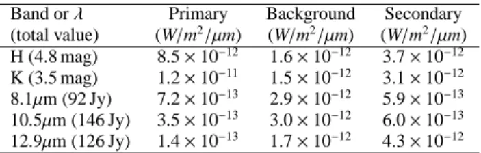
In the mid-infrared, the MIDI spectrum is close to the ISO one. Therefore, we can also assume that all the N-band flux orig-inates from the MIDI field of view (i.e ∼1”) and infer the abso-lute fluxes of the components in the N-band. These fluxes (N-band) and magnitudes (H and K-bands) are presented in Table 4 and plotted in Fig. 7 as a function of the wavelength.

Table 4. Estimated fluxes for each component from the model

fitting of Sect. 2.1.2. We used 2MASS magnitudes as the total magnitude in H and K-band and the MIDI fluxes in N-band.

Band or λ Primary Background Secondary (total value) (W/m2_/µ_m) _(W/m2_/µ_m) _(W/m2_/µ_m) H (4.8 mag) 8.5 × 10−12 _{1.6 × 10}−12 _{3.7 × 10}−12 K (3.5 mag) 1.2 × 10−11 _{1.5 × 10}−12 _{3.1 × 10}−12 8.1µm (92 Jy) 7.2 × 10−13 _{2.9 × 10}−12 _{5.9 × 10}−13 10.5µm (146 Jy) 3.5 × 10−13 _{3.0 × 10}−12 _{6.0 × 10}−13 12.9µm (126 Jy) 1.4 × 10−13 _{1.7 × 10}−12 _{4.3 × 10}−12

Even if the effect of reddening on the H and K-band flux is not negligible, a significant reddening fraction comes from the circumstellar envelope. Therefore we performed this study on the original measurements, without de-reddening.

3.4.1. A dust-enshrouded star in the South

The flux of the envelope around the southern component, from the AMBER and MIDI data, can be qualitatively described by a 1300K black body radiation (dotted line in Fig. 7). Its Gaussian FWHM, inferred from the model-fitting, is ∼4 mas (i.e. 6 AU at 1.5 kpc) in the near-infrared (H and K-bands), and is well con-strained by the AMBER 2008 data. These suggest an extended dusty envelope around this component and clearly indicate that the dust must be very close to the sublimation limit. Thus, the H and K-band emission should mainly originate from the in-ner radius of a dusty disc, encircling a viscous gas disc or a 2-component wind (Porter 2003). Estimating the envelope ex-tension with a ring instead of a Gaussian would lead to a slightly smaller size. Thus, we can estimate that the inner radius of the dusty disc is of the order of 2.5-3 AU (at 1.5 kpc).

(10)

1.0 2. 5. 10.0 20. 10−13 10−12 10−11 MIDI ISO λ (µm) Flux (W/m 2/µ m)

Fig. 7. A view of the (non-de-reddened) HD87643 SED with

the extracted fluxes from our interferometric measurements. The southern component flux is shown in red (top curve at 2 µm), the northern component flux is shown in blue (middle curve at 2 µm), and the resolved background flux is shown in pink (bot-tom curve at 2 µm). The dotted lines correspond respectively to a Kurucz spectrum of a B2V star and to a black-body flux at 1300 K, for comparison.

3.4.2. A puzzling dusty object in the North

By contrast, the northern component is unresolved (size, or di-ameter, of the source ≤ 2 mas, i.e. ≤ 3 AU at 1.5 kpc). Moreover, its flux can be accounted for neither by a simple black-body at a constant temperature nor by free-free emission. The slope of the flux variation between the H and N-bands suggests a range of temperatures for the dust (from at least ≈300 K to ≈1300 K). No cold dust can survive so close (T≈300 K at a radius ≤ 1.5 AU) to a putative luminous hot star without effective screening of the stellar radiation.

3.4.3. A cold dust circumbinary envelope

The resolved component shows a large increase of flux between H, K, and N and also carries most of the silicate emission (see Fig. 7). The binary system is therefore embedded within a large oxygen-rich, dusty envelope whose shape is not constrained by our data. This envelope must significantly contribute to the red-dening of both components.

In conclusion, we propose the following picture of the sys-tem: two stars with dusty envelopes probably surrounded by a common dusty envelope. One source might be a giant or a super-giant hot star surrounded by a disc, in which we would mainly see the inner rim corresponding to the dust sublimation radius. The other source is surrounded by a compact dusty envelope, and it is either not a luminous hot star or it is heavily screened by very close circumstellar matter. In the N-band, the circumbi-nary envelope contribution is not greater than ≈ 1”, since the MIDI (aperture 1.2”) and ISO (aperture 22×14”) fluxes match very well, and is not smaller than ≈ 200 mas, as our MIDI data indicates.

4. Concluding remarks

Our work presents new observations of HD87643, including very high angular resolution images. It completely changes the global picture of this still puzzling object:

– The binary nature of the system has been proved, with a

pro-jected physical separation of approximately 51 AU in 2008 at the adopted distance of 1.5 kpc. The orbital period is most likely several tens of years, and the large-scale nebula indi-cates a possible high eccentricity.

– The temperature of the southern component is compatible

with an inner rim of a dusty disc. In the near-IR, we do not see the central star, but it might be a giant or a supergiant star.

– The northern component and its dusty environment are

un-resolved. The underlying star is unlikely to be a massive hot star, or is heavily screened by close-by circumstellar mate-rial, as cold dust (T≈300 K) exists closer than 1.5 AU from the star (if it lies at 1.5 kpc).

– The system is embedded in a dense, circumbinary, and dusty

envelope, larger than 200 mas and smaller than 1”.

High angular resolution observations were definitely vital in partly revealing the nature of this highly intriguing object.

Therefore, we call for future observations of this system, us-ing both high spectral resolution spectroscopy and high angular resolution techniques, to place this interesting stellar system on evolutionary tracks and better understand its nature.

Acknowledgements. F. Millour and A. Meilland are funded by the Max-Planck

Institut f¨ur Radioastronomie. M. Borges Fernandes works with financial support from the Centre National de la Recherche Scientifique (France). The research leading to these results has received funding from the European Community’s Sixth Framework Programme through the Fizeau exchange visitors programme.

This research has made use of services from the CDS5_{, from the Michelson}

Science Centre6, and from the Jean-Marie Mariotti Centre7to prepare and

inter-pret the observations. Most figures in this paper were produced with the scientific

language yorick8. The authors thank K. Murakawa for fruitful discussions.

References

Allen, C. W. 1973, Astrophysical quantities (London: University of London, Athlone Press, —c1973, 3rd ed.)

Allen, D. A. & Swings, J. P. 1976, A&A, 47, 293

Baines, D., Oudmaijer, R. D., Porter, J. M., & Pozzo, M. 2006, MNRAS, 367, 737

Baron, F. & Young, J. S. 2008, in SPIE Conference series, Vol. 7013

B´echet, C., Tallon, M., Tallon-Bosc, I., & Thi´ebaut, E. 2005, in SF2A-2005: Semaine de l’Astrophysique Francaise, ed. F. Casoli, T. Contini, J. M. Hameury, & L. Pagani, 271

Bertin, E. & Arnouts, S. 1996, A&AS, 117, 393 Bjorkman, J. E. & Cassinelli, J. P. 1993, ApJ, 409, 429 Cidale, L., Zorec, J., & Tringaniello, L. 2001, A&A, 368, 160

Conti, P. S. 1997, in Astronomical Society of the Pacific Conference Series, Vol. 120, Luminous Blue Variables: Massive Stars in Transition, ed. A. Nota & H. Lamers, 161

de Freitas Pacheco, J. A., Gilra, D. P., & Pottasch, S. R. 1982, A&A, 108, 111 Domiciano de Souza, A., Driebe, T., Chesneau, O., et al. 2007, A&A, 464, 81 Haniff, C. 2006, New Astronomy Review, 51, 583

Hanson, M. M., Conti, P. S., & Rieke, M. J. 1996, ApJS, 107, 281 Hofmann, K.-H. & Weigelt, G. 1993, A&A, 278, 328

Kraus, M. 2006, A&A, 456, 151

Kraus, M. & Lamers, H. J. G. L. M. 2003, A&A, 405, 165 Kraus, S., Balega, Y. Y., Berger, J.-P., et al. 2007, A&A, 466, 649 Lamers, H. J. G. & Pauldrach, A. W. A. 1991, A&A, 244, L5

Lamers, H. J. G. L. M., Zickgraf, F.-J., de Winter, D., Houziaux, L., & Zorec, J. 1998, A&A, 340, 117

Leinert, C., Graser, U., Waters, L. B. F. M., et al. 2003, in SPIE Conference series, ed. W. A. Traub, 893–904

Leinert, C., van Boekel, R., Waters, L. B. F. M., et al. 2004, A&A, 423, 537 Lopes, D. F., Damineli Neto, A., & de Freitas Pacheco, J. A. 1992, A&A, 261,

482

5 _{http://cdsweb.u-strasbg.fr}

6 _{http://msc.caltech.edu}

7 _{http://www.jmmc.fr}

(11)

McGregor, P. J., Hyland, A. R., & Hillier, D. J. 1988, ApJ, 324, 1071 Millour, F. 2008, New Astronomy Review, 52, 177

Millour, F., Petrov, R. G., Chesneau, O., et al. 2007, A&A, 464, 107

Millour, F., Tatulli, E., Chelli, A. E., et al. 2004, in SPIE Conference series, ed. W. A. Traub., Vol. 5491 (SPIE), 1222

Millour, F., Valat, B., Petrov, R. G., & Vannier, M. 2008, in SPIE Conference series, Vol. 7013

Miroshnichenko, A. S. 1998, in Astrophysics and Space Science Library, Vol. 233, B[e] stars, ed. A. M. Hubert & C. Jaschek, 145

Miroshnichenko, A. S., Bernabei, S., Polcaro, V. F., et al. 2006, in Astronomical Society of the Pacific Conference Series, Vol. 355, Stars with the B[e] Phenomenon, ed. M. Kraus & A. S. Miroshnichenko, 347

Miroshnichenko, A. S., Levato, H., Bjorkman, K. S., et al. 2004, A&A, 417, 731 Monnier, J. D. 2006, New Astronomy Review, 51, 604

Olnon, F. M., Raimond, E., Neugebauer, G., et al. 1986, A&AS, 65, 607 Oudmaijer, R. D., Proga, D., Drew, J. E., & de Winter, D. 1998, MNRAS, 300,

170

Patience, J., Zavala, R. T., Prato, L., et al. 2008, ApJL, 674, L97 Petrov, R. G., Malbet, F., Weigelt, G., et al. 2007, A&A, 464, 1

Pojma´nski, G. 2009, in Astronomical Society of the Pacific Conference Series, Vol. 403, Astronomical Society of the Pacific Conference Series, ed. K. Z. Stanek, 52

Porter, J. M. 2003, A&A, 398, 631

Ratzka, T., Leinert, C., Henning, T., et al. 2007, A&A, 471, 173

Rousset, G., Lacombe, F., Puget, P., et al. 2003, in SPIE Conference series, ed. P. L. Wizinowich & D. Bonaccini, Vol. 4839, 140–149

Ru´e, F. & Bijaoui, A. 1997, Experimental Astronomy, 7, 129 Shore, S. N., Brown, D. N., Bopp, B. W., et al. 1990, ApJS, 73, 461 Stahl, O., Wade, G., Petit, V., Stober, B., & Schanne, L. 2008, A&A, 487, 323 Stee, P., Meilland, A., Berger, D., & Gies, D. 2005, in Astronomical Society of

the Pacific Conference Series, Vol. 337, The Nature and Evolution of Disks Around Hot Stars, ed. R. Ignace & K. G. Gayley, 211

Surdej, A., Surdej, J., Swings, J. P., & Wamsteker, W. 1981, A&A, 93, 285 Surdej, J. & Swings, J. P. 1983, A&A, 117, 359

Tatulli, E., Millour, F., Chelli, A., et al. 2007, A&A, 464, 29 Thi´ebaut, E. 2008, in SPIE Conference series, Vol. 7013

Valenti, J. A., Johns-Krull, C. M., & Linsky, J. L. 2000, ApJS, 129, 399 van den Bergh, S. 1972, PASP, 84, 594

Voors, R. H. M. 1999, PhD thesis, , Universiteit Utrecht, The Netherlands, (1999) Yudin, R. V. & Evans, A. 1998, A&AS, 131, 401

Zhao, M., Gies, D., Monnier, J. D., et al. 2008, ApJL, 684, L95 Zickgraf, F.-J. 2003, A&A, 408, 257

Zickgraf, F.-J., Wolf, B., Stahl, O., Leitherer, C., & Klare, G. 1985, A&A, 143, 421

Zorec, J. 1998, in Astrophysics and Space Science Library, Vol. 233, B[e] stars, ed. A. M. Hubert & C. Jaschek, 27

Zsarg´o, J., Hillier, D. J., & Georgiev, L. N. 2008, A&A, 478, 543

Appendix A: MIRA imaging of HD87643: tests and reliability estimates

This work made use of the MIRA software to reconstruct images from the sparsely sampled AMBER interferometric data. In this appendix, we present test results demonstrating which structures in the reconstructed images are reliable.

A.1. Altering the UV coverage

The idea here is to find out if the structures remain qualitatively the same in the final image when altering the resolution (remov-ing the high spatial frequencies) or the low frequency compo-nents of the UV plane.

A.1.1. Removing low spatial frequencies

Removing low spatial frequencies reduces the field of view, and the MIRA image reconstruction software does not manage to overcome this difficulty (see Fig. A.1). Therefore, we conclude that the low spatial frequencies (i.e. the short baselines) are just as important as longer baselines to perform image reconstruc-tion. −50 0 50 0 50 0 0.25 0.5 0.75 1 0 0.25 0.5 0.75 1 E <−−−−−−−− α (mas) δ (mas) −−−−−−−−> N −200 0 200 −200 0 200 E <−−−−−−−− sp. freq. (cycles/as) sp. freq. (cycles/as) −−−−−−−−> N

Fig. A.1. Removing low spatial frequencies to check whether

the structures are reconstructed.

A.1.2. Removing high spatial frequencies

As a second test of the image reconstruction reliability, we cut all the high spatial frequencies in order to get a more symmetric UV coverage. The result is seen in Fig. A.2, together with the corresponding UV coverage. The striking point compared to the image presented in Fig. 2 is that all the structures seen in this new image are qualitatively the same as before. This ensures that the binarity and resolution of the southern components are not due to image reconstruction artifacts.

−50 0 50 0 50 0 0.25 0.5 0.75 1 0 0.25 0.5 0.75 1 E <−−−−−−−− α (mas) δ (mas) −−−−−−−−> N −200 0 200 −200 0 200 E <−−−−−−−− sp. freq. (cycles/as) sp. freq. (cycles/as) −−−−−−−−> N

Fig. A.2. Removing high spatial frequencies to have a more

symmetric UV coverage.

A.1.3. Imaging without phases

Since the AMBER closure phases in our data-set were noisy (σ ≈ 0.5 − 1 radian), we wondered whether these phases were contributing significant information to the image reconstruction compared to squared visibilities alone.

We tried to reconstruct an image of HD87643 using the same AMBER data, except for the closure phases, and both the MIRA and BSMEM image reconstruction software. Indeed, they are able to cope with less data, in this case making a phase-retrieval image reconstruction. In Fig A.3 we show the MIRA reconstruction. We are able to reconstruct qualitatively the same image of HD87643 as in Fig. 2 without using the closure phase information.

We note, however, that we had to rotate the result to match the orientation of Fig. 2. This makes sense since only the phase information would be able to orient the system.

(12)

−50 0 50 0 50 0 0.25 0.5 0.75 1 0 0.25 0.5 0.75 1 E <−−−−−−−− α (mas) δ (mas) −−−−−−−−> N

Fig. A.3. HD87643 image reconstruction without the phase

in-formation. We had to rotate the image by 180◦_{to make it match}

the previous reconstructions.

A.2. Testing with other image reconstruction algorithms

MIRA is only one example of an image reconstruction software package for optical interferometry. Other software packages ex-ist, and we present here the tests we made using several of them.

A.2.1. BSMEM

BSMEM is based on the Maximum Entropy Method (MEM) ap-plied to bispectrum measurements (deduced from the squared visibilities and closure phase measurements). It works using an iterative algorithm, comparing the distance from the recon-structed image to the data and the “entropy” computed from the properties of the image itself (Baron & Young 2008). We applied BSMEM to the AMBER data. The result can be seen in Fig. A.4. We find the same structures as for the MIRA reconstruction pro-cess. −50 0 50 0 50 0 0.25 0.5 0.75 1 0 0.25 0.5 0.75 1 E <−−−−−−−− α (mas) δ (mas) −−−−−−−−> N

Fig. A.4. Image reconstruction of HD87643 using the BSMEM

software.

A.2.2. Building-Block Method

The Building-Block method (Hofmann & Weigelt 1993) was de-veloped to reconstruct diffraction-limited images from the bis-pectrum of the object obtained with bisbis-pectrum speckle inter-ferometry and long-baseline interinter-ferometry. Since the intensity distribution of an object can be described as a sum of many small components, the Building-Block algorithm iteratively re-constructs images by adding building blocks (e.g. δ-functions). The initial model image may simply consist of a single δ peak. Within each iteration step, the next building block is positioned

at the particular coordinate, which leads to a new model image that minimises the deviations (χ2) between the model bispectrum and the measured object bispectrum elements. An approxima-tion of the χ2_{-function was derived which allows fast calculation} of a large number of iteration steps. Adding both positive and negative building blocks, taking into account the positivity con-straint, and adding more than one building block per iteration step improves the resulting reconstruction and the convergence of the algorithm. The final image is obtained by convolving the Building-Block reconstruction with a beam matching the max-imum angular resolution of the interferometer. We applied this method to the AMBER data, and the resulting image (Fig. A.5) shows many similarities with the MIRA one, including a re-solved southern component in the K-band.

−50 0 50 0 50 0 0.25 0.5 0.75 1 0 0.25 0.5 0.75 1 E <−−−−−−−− α (mas) δ (mas) −−−−−−−−> N

Fig. A.5. Image reconstruction of HD87643 using the

Building-Block software.

A.3. Conclusion

The tests presented above show that the binary and resolved southern component are structures that can be trusted in the im-ages. All other structures (possible elongation of the southern component, inclined large “stripes” in the images) are artifacts from the image reconstruction process, which may indicate that the image has some additional flux, not constrained by the ob-servations (fully resolved background).