Drift Tube Ion Mobility: How to Reconstruct Collision Cross Section Distributions from Arrival Time Distributions?

HAL Id: hal-01639191

https://hal.archives-ouvertes.fr/hal-01639191

HAL is a multi-disciplinary open access archive for the deposit and dissemination of sci-entific research documents, whether they are pub-lished or not. The documents may come from teaching and research institutions in France or abroad, or from public or private research centers.

L’archive ouverte pluridisciplinaire HAL, est destinée au dépôt et à la diffusion de documents scientifiques de niveau recherche, publiés ou non, émanant des établissements d’enseignement et de recherche français ou étrangers, des laboratoires publics ou privés.

Distributed under a Creative Commons Attribution - NonCommercial - NoDerivatives| 4.0 International License

Drift Tube Ion Mobility: How to Reconstruct Collision

Cross Section Distributions from Arrival Time

Distributions?

Adrien Marchand, Sandrine Livet, Frederic Rosu, Valérie Gabelica

To cite this version:

Adrien Marchand, Sandrine Livet, Frederic Rosu, Valérie Gabelica. Drift Tube Ion Mobility: How to Reconstruct Collision Cross Section Distributions from Arrival Time Distributions?. Analytical Chemistry, American Chemical Society, 2017, �10.1021/acs.analchem.7b01736�. �hal-01639191�

This document is the Accepted Manuscript version of a Published Work that appeared in final form in Analytical Chemistry, copyright © American Chemical Society after peer review and technical editing by the publisher. To access the final edited and published work see

http://pubs.acs.org/doi/abs/10.1021/acs.analchem.7b01736

Drift Tube Ion Mobility: How to Reconstruct Collision

Cross Section Distributions from Arrival Time

Distributions?

Adrien Marchand1,†_{, Sandrine Livet,}1 _{Frédéric Rosu}2 _{and Valérie Gabelica}1,_*

1 _{INSERM, CNRS, Univ. Bordeaux, Laboratoire Acides Nucléiques Régulations Naturelle et}

Artificielle (ARNA, U1212, UMR5320), IECB, 2 rue Robert Escarpit, 33607 Pessac, France.

2 _{CNRS, INSERM, Univ. Bordeaux, Institut Européen de Chimie et Biologie (IECB, UMS3033,}

US001), 2 rue Robert Escarpit, 33607 Pessac, France.

† Present address: Department of Chemistry and Applied Biosciences, ETH Zürich, Switzerland. * corresponding author: Tel: +33 (0)5 4000 2940. v.gabelica@iecb.u-bordeaux.fr

Abstract: Ion mobility spectrometry allows

one to determine ion collision cross sections, which are related to ion size and shape. Collision cross sections (CCS) are usually discussed based on the peak center, yet the width of each peak contains further informa

tion on the distribution of collision cross sections of each conformational ensemble. Here, we analyze how to convert arrival time distributions (ATD) to CCS distributions (CCSD). With a calibration curve taking into account the CCS dependence of the time spent outside the mobility region, one can reconstruct CCS distributions with correct peak center values. However, the peak widths are incorrectly rendered because ion diffusion, which affects the peak width in the time domain, is irrelevant to collision cross sections. For drift tube ion mobility, we describe a new method, coined “FWHMstep”, using step-field experiment and processing the peak’s full width at half maximum to reconstruct CCSDs. The width of the CCS distributions helps to characterize the analyte’s structural heterogeneity, and/or its flexibility (i.e., the variety of ways the analyte ions can rearrange following electrospray into kinetically stable gas-phase conformations).

INTRODUCTION

Ion mobility separates ions based on their electrophoretic mobility in a buffer gas under the influence of an electric field.1-3 _{The mobility is proportional to the ion size, but also ion shape,}

and in that respect ion mobility spectrometry (IMS) is complementary to mass spectrometry. Recent technological advances have significantly improved the peak separation in ion mobility spectrometry. Resolving power values > 250 has been achieved in linear drift tubes,4 _{> 300 in}

cyclic drift tubes,5 _{up to 500 in field-assymmetric wafevorm IMS (FAIMS),}6 _{and a nominal}

resolution of ~340 was obtained with traveling wave structures for lossless ion manipulation (SLIM).7 _{The range of applications exploiting ion mobility as an additional dimension of}

separation is constantly growing, particularly towards clinical,8 _{biological and environmental}

applications.9

A common instrumental configuration involves pulsing an ion packet into the mobility device, and measuring the time ions take to reach a detector situated after the mobility cell. The primary output is thus an arrival time distribution (ATD). Beyond separation and identification based on arrival time, ion mobility spectrometry is also increasingly used to characterize ion structural ensembles, via the collision cross section (CCS).1,10-14 _{The CCS indicates the extent to which the}

ions are slowed down by collisions, and can be related to three-dimensional structural models by computation. Note that rigorously, one should call it the momentum transfer collision integral and use the symbol , but using the acronym CCS for “collision cross section” is however becoming common practice, and we will use it here for readability.

When the ATD peak width corresponds to the diffusion limit of the instrument, one generally assumes that a single structure is adopted, and it makes sense to discuss only the CCS of the center of the distribution. However, in electrospray IMS of large analytes such as peptides, proteins, and their noncovalent assemblies, peaks significantly broader than the diffusion limit are frequently observed. For example, large protein complexes can display peak widths up to 10% of the peak maximum.15 _{Slicing the broad arrival time distributions by high-resolution}

IMS-IMS demonstrates that the underlying conformational ensemble actually consists of many

distinct conformations having a continuum of CCS values.16,17 _{The width of the distributions thus}

The peak width can be represented in different ways. For example, for proteins, Bush’s group presents the CCS of the intensity-weighted center of the distribution (50% of the cumulative distribution function), and error bars are drawn using the CCS values at 10% and 90% of the cumulative distribution function.19 _{This simple representation however masks any particular}

shape of the arrival time distribution. Presenting ion mobility spectrometry results as CCS distributions (CCSD) is attractive when discussing shape, because it allows one to visually compare various molecular systems, compare results obtained on different instrumental platforms, or compare experimental and theoretical data. But despite graphs representing ion mobility results in the form of CCS distributions is becoming common in the literature, the procedure to change variables from arrival time to collision cross section is often left

undiscussed. Here we clarify the different ways to change variables, and propose a new method, based on step-field drift tube experiments, to reconstruct CCS distributions that better reflect the ion conformational ensembles.

EXPERIMENTAL METHODS

All ion mobility experiments were carried out in an Agilent 6560 drift tube IMS-Q-TOF instrument (Agilent Technologies, Santa Clara (CA), USA), with helium in the drift tube (p = 3.89 Torr, measured using an Agilent CDG-500 capacitance diaphragm gauge) and nitrogen in the collision cell (p = 2.78 × 10-5 _{Torr, measured using the instrument’s Granville Phillips}

compact ion gauge). Arrival time distributions were extracted using IM-MS Browser B.07.01 and processed with Sigmaplot 12.5. The violin plots were generated using a MatLab script (see Supporting Information).

Samples included a mixture of hexakis-(fluooalkyloxy)phosphazines (TuneMix, Agilent Technologies), bradykinin (B3259, ≥ 98%, Sigma-Aldrich, Saint Quentin-Fallavier, France), bovine ubiquitin (U6253, ≥ 98% , Sigma-Aldrich), equine cytochrome c (C7752, assay ≥ 95%, Sigma-Aldrich), bovine serum albumin (A0281, ≥ 99%, Sigma-Aldrich), deoxyribonucleic acids (RPcartridge-gold purity, Eurogentec, Seraing, Belgium) and an artificial foldamer NO2-QX7

-O-X7Q-NO2 (provided by I. Huc, University of Bordeaux).20 Tunemix was used as received. The

foldamer was sprayed from 95/5 (v:v) CHCl3/MeOH. Native proteins were prepared in aqueous

formation of 7+ ions. The polythymine mixture was sprayed from RNAse free water. The higher-order nucleic acid structures (duplexes and quadruplexes) were sprayed from aqueous

ammonium acetate (100 or 150 mM). The present article focuses on the data treatment, and the samples were selected mainly to illustrate different behaviors in terms of ion mobility peak width. More detail on sample preparation can be found in the supporting information.

THEORY

Combining the mobility equation (1) with the Mason-Schamp Equation (2) leads to equation (3), relating the time spent in the drift tube ( ) to the collision cross section (CCS):

(1)

(2)

(3)

K is the ion mobility and K0 is the reduced ion mobility, p is the pressure, p0 is the standard

pressure (760 Torr), T is the temperature, T0 is the standard temperature (273.15 K), N0 is the

buffer gas number density at T0 and p0, L is the drift tube length, tD is the drift time in the tube, E

is the electric field across the drift tube, µ is the reduced mass of the ion-gas interactions (µ =

mgas.mion/(mgas+mion)), kB is the Boltzmann constant, z is the absolute value of the ion nominal

charge, and e is the charge of the electron.

is not constant if collisions occur after the mobility region. Equation (3) or analogues are commonly seen in ion mobility articles presenting collision cross section distributions.2,21 _{If tD is}

measured directly (for example using a grid at the end of the drift tube), Eq. (3) can be used. In commercial instruments, however, the measured ion transit time is the time difference between a pulsing gate in front of the tube and a detector further away from the rear of the tube. The arrival time is the sum of the time spent in the drift cell ( ) and the time spent outside the drift cell ( ):

(4) A straightforward way to relate the experimental ATD to a CCS distribution is thus to combine Equations (3) and (4):

(5) Using Equation (5) to change variables from to CCS implicitly assumes that is independent of the CCS. This is true only for instruments that would transfer ions immediately to high

vacuum, with effectively no further collisions prior to mass analysis. However it is not true for our instrument, which has a rear funnel beyond the drift zone where V is varied, and collision cell between the IMS and the mass analyzer. Collisions occur outside the drift tube as well, and the time spent outside the drift tube thus also depends on a collision cross section. The problem with assuming that is constant is illustrated in Figure 1. Figure 1A shows the arrival time distribution of an organic foldamer molecule, containing three peaks. The collision cross section values obtained by the step-field method on each of the three peaks are 571.3, 648.2 and 724.6 Ų. The values are 5.85, 6.62 and 7.32 ms, respectively. There is no single “correct” t0 value

which would be valid for all three conformational ensembles. So, using Eq. (5) leads to different

CCS distributions depending on which peak was used to determine (Fig. 1B). Each

reconstruction is incorrectly representing the entire collision cross section distribution. The difference is visually significant, so Equation (5) is not satisfactory for rendering CCS distributions containing multiple peaks. A safer option is to present the original arrival time distributions, annotate the CCS of the center of the peaks on the figure, and tabulate CCS values separately.22,23

Figure 1. A) Arrival time distribution of an organic foldamer (z = +2) measured at V = 390.5 V. B) Collision cross section distributions reconstructed assuming that t0 is constant: in black,

using the t0 of the left peak, in blue, of the central peak and in green of the right peak. The red

annotations represent the CCS values obtained by the step-field method. C) Reconstruction obtained by applying Equation (7). The correction factor a was determined from the peak on the left (571.3 Ų), yet all peaks are positioned correctly.

How to better estimate the contribution of over the entire ATD? To reconstruct CCS distributions, one must account for the way t0 depends on the CCS. A convenient way is to

empirically correlate arrival times ( ) and CCS values for a set of ions that represent those of interest. This can be done at a single field, and must be re-done for each instrumental setting that would change either or . Traveling wave IMS calibrations follow that procedure, by

correlating arrival times ( ) with DT_{CCS values of calibrant ions in a given gas.}24

For drift tubes, combining Eq. (3) and (4) with the expression of the electric field E as a function of the voltage difference between the entrance and the exit of the IMS cell ( ∆ / ) gives:

∙√ ² _∆ (6)

One can either use known DT_{CCS values of calibrants, or determine CCS values from step-field}

experiments. We use the latter approach. The step-field experiment consists in measuring the arrival time of the center of the ATD peak ( ) as a function of (1/∆ ), and fit the data by a linear equation to obtain the CCS from the slope, according to Equation (6).

In Equation (6), (CCS.√μ/z) is related to the system, and all other terms on the right hand side depend on the instrument (length, pressure, temperature and voltage). could contain an

instrument-dependent contribution (a fixed time necessary to travel through various ion optics to the analyzer) and an analyte-dependent contribution, which could itself be related to (CCS.√μ/z) if mainly collisions are responsible for slowing down the ions on their way to the analyzer. At fixed drift voltage ∆ , let’s examine how empirically correlates with DT_CCS

He.√μ/z for a

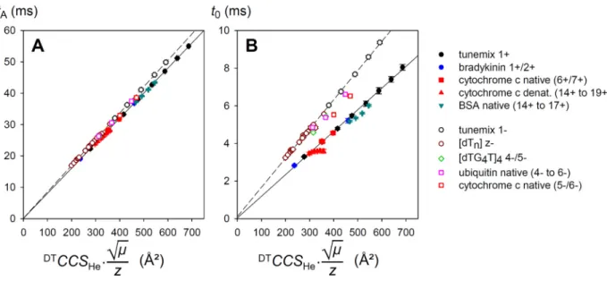
variety of cations and anions, singly or multiply charged (Figure 2A). On first approximation, the correlation is linear and goes through (0,0). But on closer examination, the data segregate

according to the analyte. Given that is strictly proportional to DT_CCS

He.√μ/z, the segregation

can only come from (Figure 2B).

First, cations and anions follow a different trendline. Because our ultimate goal is to study fragile nucleic acid non-covalent complexes, we had lowered the collision hexapole entrance and delta voltages in the negative mode, to reduce collisional activation in the collision cell (the full list of instrumental parameters is provided in the Supporting Information). For this reason, our anions take longer to reach the mass analyzer. When using the same voltage absolute values in positive

ion mode, ion transmission was lost for large proteins. However, tunemix ions could be analyzed in both modes with the same absolute voltages, and the trends superimpose (see Supporting Information Figure S1).

Figure 2. A) Arrival time ( ) measured at _{∆ = 390.5 V as a function of CCS.√μ/z}

determined from step-field experiments in helium drift tube, for various cations (filled symbols) and anions (empty symbols). See legend for the classification by compound class. The linear regressions were made using tunemix and bradykinin in positive mode, and tunemix and polythymine oligodeoxynucleotides in negative mode. The system-dependent deviation from the linear correlation comes from , as expanded in panel B). Error bars are standard deviations from three independent measurements. Note that ions were accelerated differently after the tube in positive and negative mode (IM Hex Entrance = 42 V vs. -32 V; IM Hex Delta = +8V vs. -3V, respectively).

More intriguing, even within a polarity, different molecular classes still segregate. The most striking example is that of denatured cytochrome c ions, which have lower values than the trend line given by tunemix, bradykinin, and native cytochrome c. This is rationalized as follows. In our instrument depends partly on collisions with nitrogen from the collision cell (the

mostly spent in the rear funnel), whereas depends exclusively on collisions with helium in the drift tube. The correlation between nitrogen and helium reciprocal mobilities is not linear, and depends on the ion shape.10 _{In particular, the correlation is very different for denatured proteins}

and for globular ions.26 _{To verify this interpretation, we recorded positive ion mode mobility data}

with helium both in the drift tube and in the collision cell, and found that in those conditions, denatured cytochrome c data points were no longer outliers (supporting information Figure S2). Finally, in our experimental conditions, the CCS-independent part of is negligible. Similar results were obtained by the manufacturer.27

In summary, a simple linear scaling using Equation (7) is a good approximation for changing variables between and CCS for a given system:

∙

√ (7)

In the Agilent 6560 IMS-Q-TOF, changing variables using Equation (7) renders more realistic peak positions than if assuming constant (see Figure 1C): all peak positions are rendered correctly. Again, if different gases are used in the drift tube and in the collision cell, the exact value of a will depend on the molecular nature of the ions, and not only on instrumental parameters. To determine a, knowing the CCS of the center of only one peak is sufficient. For unknowns, one will use the step-field method to determine that CCS. One can also use the CCS of a reference compound to lock the CCS scale. This is analogous to using a lock mass for internal mass calibration. Finally, note that Eq. (7) is valid only if z is the same for all species underlying the ATD. For example, its application is incorrect to deal with oligomers of different charges overlapping at a given m/z.

How to account for diffusion and extract the intrinsic width of the CCS distributions? Although the previous reconstruction properly renders the peak positions, it does not properly render the width of the CCSDs. Part of the ATD peak width is due to diffusion, and part is due to the conformational ensemble having a distribution of CCS values prior to IMS. We want to extract the latter, which is an intrinsic property of the conformational ensemble contributing to a given peak.

Each peak in the experimental ATD is fitted by a Gaussian curve. We thus here define a conformational ensemble as a collection of analyte concormations that have a Gaussian distribution of collision cross sections. Here FWHMconf will denote the contribution of the

conformational ensemble to the experimental peak width in the time domain. At each voltage, we obtain the peak center and the experimental full width at half maximum of the arrival time distribution (FWHMexp). Let’s exploit the latter.

If all ions in the ensemble have the same CCS value, the FWHM is due mainly to diffusion:

4 ln 2 _. (8)

Diffusion occurs both inside the drift tube (contributing to the width of ) and outside the drift tube (contributing to the width of ). Both contribute to the width of the distribution (i.e., of the ATD). Each can be computed if voltages are known. This is easy for the contribution inside the drift tube. The contribution to the peak width due to phenomena happening outside the drift tube (FWHMt0) is more difficult to account for: it includes contributions from the ion injection

gate28,29 _{(here, t}

gate = 100 µs in all experiments), from diffusion outside the IMS, and possibly

from electric fields outside the IMS. Assuming that the experimental ATD is a convolution of several Gaussian contributions, FWHMexp is given by:

(9)

The sum of the latter two contributions can be determined by measuring the FWHMexp of a

monomorphic compound (FWHMconf = 0) having the same charge and drift time as the analyte of

interest. This approach can be applied to traveling wave ion mobility as well,30 _{the only}

difference being the necessity to replace Eq. (7) by an equation appropriate to TWIMS to link the arrival time and CCS variables.24,31

In drift tubes, one can also use the step-field experiment to obtain the contribution of FWHMconf,

alleviating for the need for reference compounds. The first step is to subtract the in-IMS contribution (easy to compute from Eq. (8) in DTIMS) from the experimental FWHM, to calculate , which is thus the convolution of the contributions of the analyte and of peak broadening outside the drift region (Eq. 10):

(10)

The contribution outside the IMS is by definition independent of the drift tube voltage V. Thus, any change in along the step-field experiment is related to the analyte’s

conformational heterogeneity.

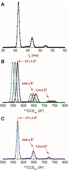
Reconstructing the CCS distribution means finding not only the CCS of the center of the peak, but also the CCS of the ions that drifted faster (smaller CCS) or slower (larger CCS) than the center of the peak. We will illustrate the method with the arrival time distributions of the G-quadruplex [dTG4T]45- (Figure 3). Figure 3B shows the linear regression as a function of 1/ for

the arrival time of the peak ceter _, , which according to the usual step-field procedure (Eq. (6)) gives . We do the same for ions with arrival times at half-maximum of the

peak, using ( _, /2). The contributions outside the IMS contribute to the

intercept, but not to the slope. Thus the change of slopes of these two new linear regressions is due only to the contribution of the different CCS values across the conformational ensemble. In other words, the two new CCS values obtained from the two new slopes are equal to

/2. We thus obtain , the width of the CCS distribution,

and can construct a Gaussian CCS distribution that contains only the contributions of the conformational heterogeneity of the ensemble (Figure 3D).

The procedure explained above is easier to understand intuitively. However it is faster, mathematically equivalent, and more accurate (lower error propagation) to fit directly the

FWHMstep values as a function of 1/V. Also, the residuals and the quality of the fit are easier to

assess visually. The is directly obtained from the slope of FWHMstep as a function of

1/V (see Fig. 3C), following Eq. (11), itself derived from Eq. (6):

∙√ ²

Figure 3. A) Arrival time distribution for the DNA tetramolecular G-quadruplex [dTG4T]45- at

five different V values (390, 490, 590, 690 and 790 V, in cyan, red, green, brown and black, respectively). The Gaussian curves were obtained by fitting the experimental ATDs, and were normalized based on their area. B) Arrival time versus 1/V for the peak center and tA, center ± ½

FWHMstep. Inserts show the fitting of the three series of points and their respective intercept (t0).

C) How the experimental peak width at half maximum (FWHMexp, full bar) and FWHMstep (blue

portion of the bar) vary with 1/V. The solid line shows the linear fit from which FWHMCCS is

obtained from the slope, and the FWHMt0 is obtained from the intercept. D) Reconstructed CCS

distributions. Black: data points converted using Equation (5) with V = 390.5 V (reconstruction at all drift voltages, see Supporting Figure S3A). Blue: data points converted using Equation (7) with V = 390.5 V (reconstruction at all drift voltages, see Supporting Figure S3B). Red: Gaussian curve reconstructed with the “FWHMstep” method.

RESULTS

Figure 3 illustrates the resconstruction for the DNA tetramolecular G-quadruplex [dTG4T]45-,

which has a narrow arrival time distribution (resolving power ( / ) 56 at 390.5 V). When reconstructed with Equation (7), the apparent / is naturally identical. Nevertheless, it is still unduly broad. Figure 3C shows how FWHMexp and FWHMstep change

with 1/V for [dTG4T]45-. We can see that the diffusion inside IMS contributed significantly to

the peak width in the time domain (red bar). Besides, peak broadening outside the IMS is not negligible either ( = 257 ± 17 µs). When the inherent width of the CCS distribution of the conformational ensemble is obtained from the FWHMstep method, the relative is 0.7% of the center CCS (the equivalent “resolution” would be over 150).

The narrow distribution is attributed to the rigidity of the parallel G-quadruplex stem.13 _Other

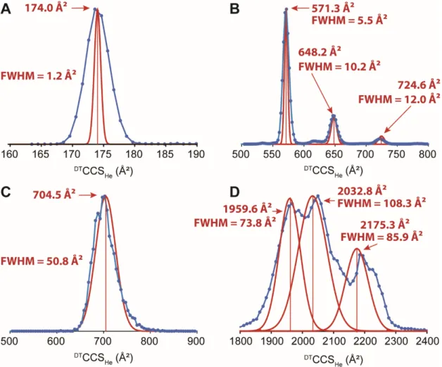
examples of narrow CCS distributions are shown in Figures 4A (tunemix, m = 922 and z = 1) and 4B (the foldamer of Figure 1). The blue distributions are reconstructed using Eq. (7), with the proportionality factor a determined from the center of the most intense peak, and the red distributions are Gaussian curves reconstructed with the “FWHMstep” method. The linear

regressions on the peak widths are shown in Supporting Information Figure S4. The relative peak widths at half maximum ( / ) are 0.7 % for the tunemix ion 922, and 1.0 % for the foldamer main peak.

Fig. 4C illustrates the processing of a broad ATD, recorded with the DNA duplex [dCGCGGGCCCGCG]25-. Duplexes are less rigid than parallel G-quadruplexes such as

[dTG4T]45-. They collapse into a variety of structures by forming extra phosphate-phosphate

hydrogen bonds upon desolvation and declustering, and the various collapsed structures do not interconvert after desolvation.32 _{The CCS distribution reconstructed with the “FWHMstep”}

method is as broad as the one reconstructed using Eq. (7). Its relative width at half-maximum is 7.2 %. One may argue that the absolute contribution of the diffusion differs on both ends of the peaks when the CCS values differ so much. However, the relative contribution of the diffusion to the peak width is very small (see supporting Figure S4), thus this is a very minor source of error.

Figure 4. Examples of reconstructed CCS distributions. Blue: data points converted using

Equation (7). Red: Gaussian curves reconstructed with the “FWHMstep” method. A)

Tunemix ion at m = 922 and z = 1. B) Foldamer [NO2-QX7-O-X7Q-NO2]2+. C) DNA duplex

[dCGCGGGCCCGCG]25-. D) denatured [cytochrome c]10+.

Finally, Fig. 4D illustrates the output of the “FWHMstep” method on a more complex arrival time distribution ([cytochrome c]10+ _{produced from denaturing solution conditions). The}

experimental arrival time distribution at our lowest drift voltage (V = 390.5 V) shows four peaks, the one at the longest arrival time being a shoulder of the penultimate peak. However, the two slowest peaks are not resolved at every drift voltage, so we could not apply the FWHMstep method to all four peaks, and thus fitted the last two peaks by a single Gaussian function. This illustrates one limitation of our method: the same peaks must be resolved at all drift voltages of the step-field experiment. The three reconstructed Gaussian curves have different widths, and

this provides information on the polydispersity of each resolvable ensemble. We also see that the positions of the peaks obtained by applying Eq. (7) on the first peak (blue curve) are not the same as when using the step-field method. As we saw in Figure 2, different protein

conformations have different dependences on the helium CCS. The step-field reconstructions (in red) are the correct peak positions.

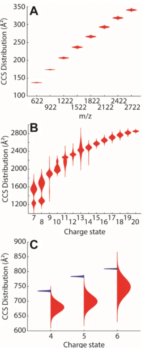
The reconstructed CCS distributions can be used to build violin plots (Figure 5), which are useful to visually compare peak centers and peak widths simultaneously. The violin plots show a

distribution along the vertical axis, for different datasets on the horizontal axis. When only one series is shown, the distribution is presented with its mirror image to create the violin. For example, the evolution of CCS as a function of size is often used to determine if the structure grows following an isotropic or linear law, hinting at spherical or rod-like structures,

respectively.33 _{Traditional plots show points corresponding to the CCS of the peak center. Figure}

5A illustrates this for tunemix ions. The peak width is useful to determine the goodness of a fit, and whether a data point is an outlier or not. Another frequent data visualization is the CCS as a function of the charge state. Such graphs usually display dots.2 _{Figure 5B shows the violin plot}

of denatured cytochrome c (as the sum of the reconstructed Gaussian curves), which adds visual information on the relative abundances of each ensemble, and on their intrinsic polymorphism. Finally, asymmetric violin plots (one distribution towards the left, one towards the right) facilitate comparisons between two systems or conditions. Figure 5C shows how two DNA structures with the same size (24 nucleobases) compare. The violin plot highlights

simultaneously the difference in CCS values, the charge dependence, and the width of the distribution.

Figure 5. Violin plots of CCS distributions reconstructed with the FWHMstep method. The

y-axis is the CCS distribution of the ion labeled on the x-y-axis. For single series (A and B), the mirrored CCS distribution is represented. To visually compare two series (C), different

distributions are plotted on the left and on the right. A) size dependence of CCS for tunemix in positive mode. B) Charge state dependence for denatured cytochrome c in positive mode. C)

Comparison between two DNA systems containing 24 nucleobases: (red) the duplex

[dCGCGGGCCCGCG]2 and (blue) the G-quadruplex [dTG4T]4, for several charge states in

DISCUSSION

A significantly large means that the ion population under a given peak adopts a variety of gas-phase conformations, presenting a distribution of CCS values which is also Gaussian. A Gaussian distribution is the most probable distribution that can be assumed in the absence of resolvable peak shoulders in the ATD. If a shoulder is resolved by a peak fitting software at all fields of the step-field experiment, then it is treated as a separate ensemble. The necessity to obtain quality fits of the ATD can limit the applicability of our method to complex distributions. Peak shoulders are not necessarily resolvable at all fields. For complex ATDs, using Eq. (7) remains the back-up plan, despite not taking some sources of broadening into account. Complex ATD’s are usually much broader than those of monomorphic analytes would be, and we showed that in such cases (e.g., the duplex) the magnitude of the correction to the peak width offered by the FWHMstep method is small. Remember also that when different gases are used inside and outside the drift tube, the peak positions may not be rendered correctly. Another case of complex ATD consists of species with different charges z (for example, m/z-overlapped oligomers). Here, a different Gaussian CCSD must be reconstructed for each peak, using the appropriate z value. This is however difficult if the peaks overlap.

We also note that the Gaussian distribution of CCS values is valid only for systems that do not interconvert in the drift tube. If interconversion occurs on the time scale of the mobility

separation, kinetic modeling is required to account for the shape of the arrival time

distribution.34-36 _{When inter-conversion is at least 10 times faster than the time scale of mobility}

separation, the entire ion population drifts with the same average time, and the distribution is as narrow as a diffusion-limited ATD would be.36 _{Thus, a significantly broad peak indicates an}

intrinsic distribution of CCS values prior to entrance in the drift cell, and that these conformations do not interconvert at the temperature and time scale at which ion mobility separation is conducted.

Our procedure doesn’t take into account the contribution of space charge. We initially thought that space charge was the reason why we don’t find CCS distributions closer to dirac functions, even for the tunemix ions that show very narrow ATDs in super-resolution SLIM (structures for lossless ion manipulation) devices.37 _{Our drift tube instrument being placed right after the}

in the ion accumulation region. However, control experiments at lower concentrations and ion intensities led to the same peak widths. The narrowest peaks we obtain have a FWHMCCS  1%

of the peak center. This is narrower than with the highest resolving power obtainable in helium (~56 for a 5- charge state). We however have not uncovered yet why this error is always positive (not centered around zero-width), i.e. why for the presumably monomorphic tunemix ions the slopes FWHMstep/ (1/V) are systematically positive and not equal to zero. Further

investigation of the field effect on the peak width would be needed. In Figure S4, the standard error on the slope is rather constant throughout the dataset (15-30 ms/V-1_{), which translates into}

an error on the FWHMCCS of 1.5 to 3 Ų. In relative terms, the error on the reconstructed width is

substantial for narrow peaks only.

Although our procedure is not quantitatively perfect, it already better reflects the width of the CCS distribution, compared to Eq. (5) or (7). With these two equations, the reconstructed width depends on the resolving power and thus on the drift voltage (Supporting Information Figure S3). Also, in contrast with the procedure recently described by Kune et al.,30 _{we make no}

assumption with regard to the number of conformations hidden under an ATD which is broader than if just diffusion-limited. Here, we treat each Gaussian ATD peak as an ensemble, each having a distribution of CCS values.

CONCLUSION

In summary, we propose a new data processing method for step-field drift tube ion mobility experiments, to extract the width of the CCS distribution (CCSD) of each conformational ensemble, in addition to the average CCS values of each ensemble. The new “FWHMstep” method allows one to reconstruct CCSDs more faithfully, to visually compare different systems, different experimental conditions, or to compare experimental and theoretical CCS distributions instead of singular CCS values. For narrow peaks observed at the limits of our commercial drift tube’s resolving power in helium (~56), the reconstructed CCSDs had peak widths of less than 1% of the half-maximum. Thus, reconstructed distributions broader than 1% of the peak center indicate that ion populations consist of heterogeneous conformational ensembles, which do not interconvert on the time scale of the mobility separation. We also propose using violin plots of

the reconstructed collision cross section distributions to visualize trends in collision cross sections, both for the peak center and for the peak width.

ASSOCIATED CONTENT Supporting Information

The Supporting Information is available free of charge on the ACS Publications website: Instrument tuning parameters, detailed sample preparation, list of tA, t0 and CCS values of

Figure 2, t0 and CCS values in positive and negative mode with other collision cell voltages,

and with helium in the collision cell, additional arrival time distributions and CCS distribution reconstructions, Matlab scripts to create the violin plots. (PDF)

AUTHOR INFORMATION Corresponding Author

* Valérie Gabelica, IECB, 2 rue Robert Escarpit, 33607 Pessac, France. Tel: +33 (0)5 4000 2940. Email: v.gabelica@iecb.u-bordeaux.fr.

Present Addresses

† Department of Chemistry and Applied Biosciences, ETH Zürich, Switzerland.

Author Contributions

AM and VG conceived the research, SL and FR collected data, AM, SL, FR and VG treated the data and interpreted the results. AM and VG wrote the manuscript. All authors have given approval to the final version of the manuscript.

ACKNOWLEDGEMENTS

This work was supported by the Inserm (ATIP-Avenir Grant no. R12086GS), the Conseil

Régional Aquitaine (Grant no. 20121304005), and the EU (FP7-PEOPLE-2012-CIG-333611 and ERC-2013-CoG-616551-DNAFOLDIMS). We acknowledge Ivan Huc (IECB Bordeaux) for donating the foldamer sample and Nora Nowak (ETH Zurich) for help in writing MatLab scripts.

REFERENCES

(1) Wyttenbach, T.; Bowers, M. T. Mod. Mass Spectrom. 2003, 225, 207-232.

(2) Bohrer, B. C.; Merenbloom, S. I.; Koeniger, S. L.; Hilderbrand, A. E.; Clemmer, D. E. Annu.

Rev. Anal. Chem. 2008, 1, 293-327.

(3) Clemmer, D. E.; Jarrold, M. F. J. Mass Spectrom. 1997, 32, 577-592. (4) Groessl, M.; Graf, S.; Knochenmuss, R. Analyst 2015, 140, 6904-6911.

(5) Merenbloom, S. I.; Glaskin, R. S.; Henson, Z. B.; Clemmer, D. E. Anal. Chem. 2009, 81, 1482-1487.

(6) Shvartsburg, A. A.; Seim, T. A.; Danielson, W. F.; Norheim, R.; Moore, R. J.; Anderson, G. A.; Smith, R. D. J. Am. Soc. Mass Spectrom. 2013, 24, 109-114.

(7) Deng, L.; Webb, I. K.; Garimella, S. V. B.; Hamid, A. M.; Zheng, X.; Norheim, R. V.; Prost, S. A.; Anderson, G. A.; Sandoval, J. A.; Baker, E. S.; Ibrahim, Y. M.; Smith, R. D. Anal. Chem.

2017, 89, 4628-4634.

(8) Chouinard, C. D.; Wei, M. S.; Beekman, C. R.; Kemperman, R. H.; Yost, R. A. Clin. Chem.

2016, 62, 124-133.

(9) Zheng, X.; Wojcik, R.; Zhang, X.; Ibrahim, Y. M.; Burnum-Johnson, K. E.; Orton, D. J.; Monroe, M. E.; Moore, R. J.; Smith, R. D.; Baker, E. S. Annu. Rev. Anal. Chem. 2017, 10, 71-92. (10) Bush, M. F.; Hall, Z.; Giles, K.; Hoyes, J.; Robinson, C. V.; Ruotolo, B. T. Anal. Chem.

2010, 82, 9557-9565.

(11) Jurneczko, E.; Barran, P. E. Analyst 2011, 136, 20-28.

(12) Marklund, E. G.; Degiacomi, M. T.; Robinson, C. V.; Baldwin, A. J.; Benesch, J. L.

Structure 2015, 23, 791-799.

(13) D'Atri, V.; Porrini, M.; Rosu, F.; Gabelica, V. J. Mass. Spectrom. 2015, 50, 711-726. (14) May, J. C.; Morris, C. B.; McLean, J. A. Anal. Chem. 2017, 89, 1032-1044.

(15) Uetrecht, C.; Rose, R. J.; van, D. E.; Lorenzen, K.; Heck, A. J. Chem. Soc. Rev. 2010, 39, 1633-1655.

(16) Koeniger, S. L.; Merenbloom, S. I.; Clemmer, D. E. J. Phys. Chem. B 2006, 110, 7017-7021.

(17) Allen, S. J.; Eaton, R. M.; Bush, M. F. Anal. Chem. 2017, 89, 7527-7534. (18) Maurer, M. M.; Donohoe, G. C.; Valentine, S. J. Analyst 2015, 140, 6782-6798. (19) Laszlo, K. J.; Munger, E. B.; Bush, M. F. J. Phys. Chem. B 2017, 121, 2759-2766. (20) Li, X.; Qi, T.; Srinivas, K.; Massip, S.; Maurizot, V.; Huc, I. Org. Lett. 2016, 18, 1044-1047.

(21) Shi, L.; Holliday, A. E.; Shi, H.; Zhu, F.; Ewing, M. A.; Russell, D. H.; Clemmer, D. E. J.

Am. Chem. Soc. 2014, 136, 12702-12711.

(22) Ujma, J.; De Cecco, M.; Chepelin, O.; Levene, H.; Moffat, C.; Pike, S. J.; Lusby, P. J.; Barran, P. E. Chem. Commun. 2012, 48, 4423-4425.

(23) Bleiholder, C.; Do, T. D.; Wu, C.; Economou, N. J.; Bernstein, S. S.; Buratto, S. K.; Shea, J. E.; Bowers, M. T. J. Am. Chem. Soc. 2013, 135, 16926-16937.

(24) Ruotolo, B. T.; Benesch, J. L.; Sandercock, A. M.; Hyung, S. J.; Robinson, C. V. Nat.

Protoc. 2008, 3, 1139-1152.

(25) Ibrahim, Y. M.; Baker, E. S.; Danielson, W. F., 3rd; Norheim, R. V.; Prior, D. C.; Anderson, G. A.; Belov, M. E.; Smith, R. D. Int. J. Mass Spectrom. 2015, 377, 655-662.

(26) Bleiholder, C.; Johnson, N. R.; Contreras, S.; Wyttenbach, T.; Bowers, M. T. Anal. Chem.

2015, 87, 7196-7203.

(27) Stow, S. M.; Causon, T. J.; Zheng, X.; Kurulugama, R. T.; Mairinger, T.; May, J. C.; Rennie, E. E.; Baker, E. S.; Smith, R. D.; McLean, J. A.; Hann, S.; Fjeldsted, J. C. Anal. Chem.

2017, 89, 9048-9055.

(28) Siems, W. F.; Wu, C.; Tarver, E. E.; Hill, H. H.; Larsen, P. R.; McMinn, D. G. Anal. Chem.

(29) Wu, C.; Siems, W. F.; Asbury, G. R.; Hill, H. H. Anal. Chem. 1998, 70, 4929-4938. (30) Kune, C.; Far, J.; De Pauw, E. Anal. Chem. 2016, 88, 11639-11646.

(31) Shvartsburg, A. A.; Smith, R. D. Anal. Chem. 2008, 80, 9689-9699.

(32) Porrini, M.; Rosu, F.; Rabin, C.; Darre, L.; Gomez, H.; Orozco, M.; Gabelica, V. ACS Cent.

Sci. 2017, 3, 454-461.

(33) Bleiholder, C.; Dupuis, N. F.; Wyttenbach, T.; Bowers, M. T. Nature Chem. 2011, 3, 172-177.

(34) Kinnear, B. S.; Hartings, M. R.; Jarrold, M. F. J. Am. Chem. Soc. 2001, 123, 5660-5667. (35) Kohtani, M.; Jones, T. C.; Sudha, R.; Jarrold, M. F. J. Am. Chem. Soc. 2006, 128, 7193-7197.

(36) Poyer, S.; Comby-Zerbino, C.; Choi, C. M.; MacAleese, L.; Deo, C.; Bogliotti, N.; Xie, J.; Salpin, J. Y.; Dugourd, P.; Chirot, F. Anal. Chem. 2017, 89, 4230-4237.

(37) Deng, L.; Ibrahim, Y. M.; Hamid, A. M.; Garimella, S. V.; Webb, I. K.; Zheng, X.; Prost, S. A.; Sandoval, J. A.; Norheim, R. V.; Anderson, G. A.; Tolmachev, A. V.; Baker, E. S.; Smith, R. D. Anal. Chem. 2016, 88, 8957-8964.