HAL Id: tel-03171608
https://hal.archives-ouvertes.fr/tel-03171608
Submitted on 17 Mar 2021
HAL is a multi-disciplinary open access archive for the deposit and dissemination of sci-entific research documents, whether they are pub-lished or not. The documents may come from teaching and research institutions in France or abroad, or from public or private research centers.
L’archive ouverte pluridisciplinaire HAL, est destinée au dépôt et à la diffusion de documents scientifiques de niveau recherche, publiés ou non, émanant des établissements d’enseignement et de recherche français ou étrangers, des laboratoires publics ou privés.
E. S. G. de Almeida
To cite this version:
E. S. G. de Almeida. Disks and winds around hot stars: new insights from multi-wavelength spec-troscopy and interferometry. Solar and Stellar Astrophysics [astro-ph.SR]. Université Côte D’Azur, 2020. English. �NNT : 2020COAZ4074�. �tel-03171608�
apport de la spectroscopie et de l’interférométrie
multi-bandes
Elisson SALDANHA DA GAMA DE ALMEIDA
Laboratoire J.-L. Lagrange (UMR 7293), Observatoire de la Côte d’AzurPrésentée en vue de l’obtention du grade de docteur en
Sciences de la Planète et de l’Univers
de l’Université Côte d’Azur
Thèse dirigée par Armando DOMICIANO DE SOUZA et par Anthony MEILLAND
Soutenue le : 23 novembre 2020 Devant le jury composé de :
Alex CARCIOFI, Professeur, IAG/USP, São Paulo, Brasil
Anthony MEILLAND, Chercheur CR CNRS, Laboratoire Lagrange/OCA, UCA, Nice
Armando DOMICIANO DE SOUZA, Astronome Adjoint, Laboratoire Lagrange/OCA, UCA, Nice Bruno LOPEZ, Astronome, Laboratoire Lagrange/OCA, UCA, Nice
Evelyne ALECIAN, Chercheur CR CNRS, Université Grenoble Alpes, Grenoble
Jean-Claude BOURET, Chercheur DR CNRS, Laboratoire d'Astrophysique de Marseille, Marseille Marcelo BORGES FERNANDES, Professeur, Observatório Nacional, Rio de Janeiro, Brasil Philippe STEE, Chercheur DR CNRS, Laboratoire Lagrange/OCA, UCA, Nice
apport de la spectroscopie et de l’interférométrie
multi-bandes
Jury :
Président du jury :
Marcelo BORGES FERNANDES, Professeur, Observatório Nacional, Rio de Janeiro, Brasil
Rapporteurs :
Evelyne ALECIAN, Chercheur Chargé de Recherche CNRS, Université Grenoble Alpes, Grenoble Marcelo BORGES FERNANDES, Professeur, Observatório Nacional, Rio de Janeiro, Brasil
Examinateurs :
Alex CARCIOFI, Professeur, Instituto de Astronomia, Geofísica e Ciências Atmosféricas/ Universidade de São Paulo, São Paulo, Brasil
Bruno LOPEZ, Astronome, Laboratoire Lagrange/Observatoire de la Côte d’Azur, Université Côte d’Azur, Nice
Jean-Claude BOURET, Chercheur Directeur de Recherche CNRS, Laboratoire d'Astrophysique de Marseille, Marseille
Philippe STEE, Chercheur Directeur de Recherche CNRS, Laboratoire Lagrange/Observatoire de la Côte d’Azur, Université Côte d’Azur, Nice
Invités :
Sylvia EKSTRÖM, Docteur, Observatoire Astronomique de l’Université de Genève
Directeur :
Armando DOMICIANO DE SOUZA, Astronome Adjoint, Laboratoire Lagrange/Observatoire de la Côte d’Azur, Université Côte d’Azur, Nice
Co-directeur :
Anthony MEILLAND, Chercheur Chargé de Recherche CNRS, Laboratoire Lagrange/Observatoire de la Côte d’Azur, Université Côte d’Azur, Nice
I would like to thank my advisors, Armando Domiciano de Souza and Anthony Meilland, for all their support, commitment with my work, and for introducing me to the interferometric journey of hot stars. I also thank you for helping me with the practical stuff of life during my stay in Nice. Thank you a lot for helping me with the heavy baggage when I arrived in Nice !
I thank Yves Rabbia for sharing his time to teach me the theory of stellar interfe-rometry, and also Denis Mourard and Frédéric Morand for giving me the opportunity to learn about interferometric observations with the CHARA/VEGA instrument at Plateau de Calern. I thank Alain Spang for working on the reduction of new VLTI/AM-BER data of Rigel (and also for your occasional visits to my office and nice handshakes), Farrokh Vakili for inviting me to study P Cygni using intensity interferometry, and Philippe Stee for participating of my PhD meetings with Armando and Anthony (also for your constructive comments on my paper about 𝑜 Aquarii). Philippe and Farrokh, thank you very much for reading and commenting on my thesis manuscript ! I also thank Christine Delobelle, Delphine Saissi, and Sophie Rousset for helping me with the french bureaucracy.
I thank Julieta Sanchez, Fei Hua, and Mircea Moscu for sharing with me good moments during my stay in Nice. Julieta, thank you very much for receiving me at your home in La Plata. Also many thanks for Alban Ceau, Marc-Antoine Martinod, Pierre Janin-Potiron, Romain Laugie, and Vicent Hocdé : thank you for being patient with my French. I hope to meet all you again to have a glass of beer or a cup of coffee. Massinissa Hadjara, thank you for being a very nice neighbor and for the good green grapes !
I would like to thank Alex Carciofi, Bruno Lopez, Evelyne Alecian, Jean-Claude Bouret, Marcelo Borges, Philippe Stee, and Sylvia Ekström for being part of the jury of my thesis and for their constructive comments on my work. Em português, agradeço
me ajudar com os preparativos da defesa online no Observatório Nacional.
Agradeço aos meus pais, Elionai e Sônia, e minha tia Lila, por todo amor e apoio desde sempre. Também aos melhores amigos do mundo : David Campos, Icaro Rossi-gnoli, Marcio Monteiro, Morgana Romão e Poema Portela. Muito obrigado por estarem sempre ao meu lado em todos os momentos, seja online ou de forma presencial. Obri-gado também por suportarem minhas reclamações. Poema e Marcio, obriObri-gado por me visitarem em Nice ! Pai, mãe e tia Lila, a visita de vocês também está guardada para sempre comigo com muito carinho. Também deixo meu agradecimento à Alinges Lenz pela escuta recente e pelo incentivo para seguir em frente.
Hot stars are the main source of ionization of the interstellar medium and its enrichment due to heavy elements. Constraining the physical conditions of their environments is crucial to understand how these stars evolve and their impact on the evolution of galaxies.
Spectroscopy allows to access the physics, the chemistry, and the dynamics of these objects, but not the spatial distribution of these objects. Only long-baseline interferometry can resolve photospheres and close environments, and, combining spectroscopy and interferometry, spectro-interferometry allows to draw an even more detailed picture of hot stars.
The objective of my thesis was to investigate the physical properties of the photosphere and circumstellar environment of massive hot stars confronting multi-band spectroscopic or spectro-interferometric observations and sophisticated non-LTE radiative transfer codes.
My work was focused on two main lines of research. The first concerns radiative line-driven winds. Using UV and visible spectroscopic data and the radiative transfer code CMFGEN, I investigated the weak wind phenomenon on a sample of nine Galactic O stars. This study shows for the first time that the weak wind phenomenon, originally found for O dwarfs, also exists on more evolved O stars and that future studies must evaluate its impact on the evolution of massive stars.
My other line of research concerns the study of classical Be stars, the fastest rotators among the non-degenerated stars, and which are surrounded by rotating equatorial disks. I studied the Be star 𝑜 Aquarii using H𝛼 (CHARA/VEGA) and Br𝛾 (VLTI/AMBER) spectro-interferometric observations, the radiative transfer code HDUST, and developing new automa-tic procedures to better constrain the kinemaautoma-tics of the disk. This multi-band study allowed to draw the most detailed picture of this object and its environment, to test the limits of the current generation of radiative transfer models, and paved the way to my future work on a large samples of Be stars observed with VEGA, AMBER, and the newly available VLTI mid-infrared combiner MATISSE.
Keywords :stars : massive, emission-line, atmospheres, winds, circumstellar matter ; tech-niques : spectroscopic, interferometric.
Les étoiles chaudes sont la principale source d’ionisation du milieu interstellaire et de son enrichissement en éléments lourds. Contraindre les conditions physiques de leur environnement est crucial pour comprendre comment ces étoiles évoluent et leur impact sur l’évolution des galaxies.
La spectroscopie permet d’accéder à la physique, la chimie et la dynamique de ces objets, mais pas à la distribution spatiale de ces objets. L’interférométrie à longue base est la seule technique permettant de résoudre la photosphère et les environnements, et, en combinant spectroscopie et interférométrie, la spectro-interférométrie permet de dresser une image encore plus détaillée des étoiles chaudes.
L’objectif de ma thèse était d’étudier les propriétés physiques de la photosphère et de l’environnement circumstellaire d’étoiles chaudes massives, en confrontant des observations spectroscopiques et spectro-interférométriques sur différents domaines de longueur d’onde à des modèles sophistiqués de transfert radiatif hors-ETL.
Mon travail s’est focalisé sur deux axes. La première concerne les vents radiatifs. En utilisant des données spectroscopiques UV et visible et le code CMFGEN, j’ai étudié le phénomène des vents faibles sur un échantillon de neuf géantes O galactiques. Cette étude montre pour la première fois que le phénomène des vents faibles, trouvé à l’origine pour les naines O, existe également pour des étoiles O plus évoluées et que des prochaines études doivent évaluer leur effet sur l’évolution des étoiles massives.
Mon autre axe de recherche concerne l’étude des étoiles Be classiques, les rotateurs les plus rapides parmi les étoiles non dégénérées et qui sont entourées par des disques équatoriaux en rotation. J’ai étudié l’étoile Be 𝑜 Aquarii en utilisant des données spectro-interférométriques obtenues en H𝛼 (CHARA/VEGA) et Br𝛾 (VLTI/AMBER), le code de transfert radiatif HDUST, et en développant de nouvelles procédures automatiques pour mieux contraindre la cinématique des disques. Cette étude multi-bande a permis d’obtenir la vue la plus complète de cet objet et de son environnement, de tester les limites de la génération actuelle de modèles de transfert radiatif, et d’ouvrir la voie à des travaux futurs sur un échantillon large d’étoiles Be observées avec VEGA, AMBER et MATISSE, le nouvel instrument infrarouge thermique du VLTI.
Mots-clés : étoiles : massive, raie d’émission, atmosphères, vents, matière circumstellaire ; techniques : spectroscopique, interférométrique.
1.1 Schemes of chemical stratification in evolved massive stars (left) and evolved low-intermediate-mass (right) stars. . . 4 1.2 Modified Conti scenario for the evolutionary scheme of massive stars as
a function of zero-age main sequence mass. . . 5 1.3 Mass-loss rate (left axis, solid line) and stellar mass (right axis, dashed
line) as function of age in the Geneva evolutionary model for a non-rotating single star with MZAMS = 60 M⊙. . . 6
1.4 The R136 open cluster located in the H ii region 30 Doradus (Tarantula Nebula) in the Large Magellanic Cloud. . . 7 1.5 Mass return rate (logarithmic scale) of massive stars as a function of
stellar mass. . . 8 1.6 Amount of dust mass produced by AGB stars and supernovae as a
func-tion of progenitor initial mass from Gall et al. (2011b). . . 9 1.7 Minimum MZAMS that allows a complete stellar evolution at a certain
value of cosmological redshift (𝑧). . . 10 1.8 Schematic representation of iteration between a photon with linear
mo-mentum ℎ𝜈/𝑐 (energy given by ℎ𝜈) and a particle of mass 𝑚. . . 16 1.9 Ultraviolet spectrum of the O supergiant (type O9.5I) IC 1613-B11
(lo-cated in the dwarf galaxy IC 1613) is shown in black line. . . 19 1.10 Fraction of the radiative acceleration due to each chemical element,
compared with the total radiative force (𝑎rad), as a function of distance
from the star, in the PoWR model of Sander et al. (2017) to the analysis of 𝜁 Puppis. . . 21 1.11 Comparison between a initial smooth wind structure (dashed line,
mo-dified CAK-theory) and one predicted from time-dependent hydrodyna-mical simulation from Puls et al. (1993) after 60000 s (solid line) . . . . 24 1.12 Mass-loss rate as a function of stellar luminosity at different evolutionary
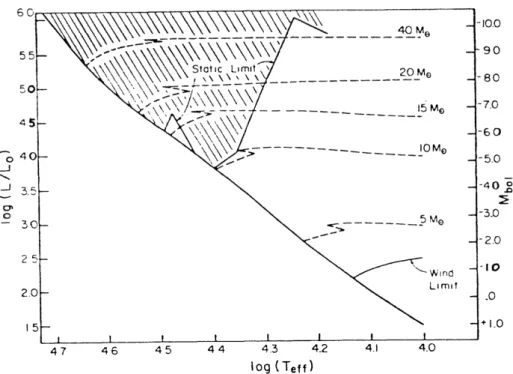
stages of massive stars. . . 25 1.13 Limits in the HR diagram for acceleration winds due to lines. . . 27
1.14 Boxplot distribution of the projected stellar rotation velocity (𝑣 sin 𝑖) as a function of spectral type. . . 28 1.15 Gravity darkening and geometrical oblateness effects due to rotation. . 35 1.16 Temporal evolution of the linear stellar equatorial velocity (left panel)
from Geneva evolutionary models for massive stars with different initial masses. The corresponding angular rotational rate is shown in the right panel. . . 36 1.17 Rotational rate 𝑊 of Be-type stars as a function of effective temperature
from different studies in the literature. . . 37 1.18 Comparison between the fraction of stars rotating faster than a minimum
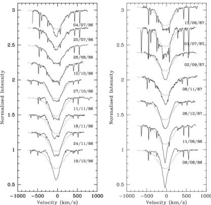
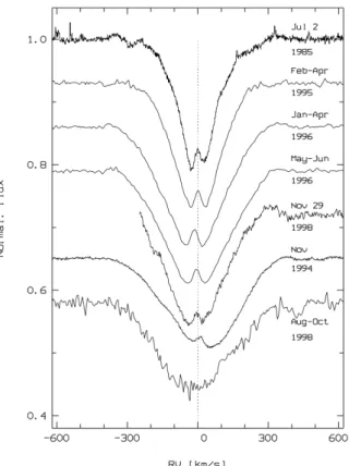
value (theoretical fraction in color lines) and the observed fraction of Be stars in Galatic clusters (left panel). . . 38 1.19 Struve’s picture to explain the emission line profiles of Be stars. . . 41 1.20 Temporal variation from 1986 to 1988 of the observed H𝛼 profile (solid
black lines) of 𝑜 Andromedae (B6IIIpe). . . 42 1.21 Temporal variability of the CQE feature in the He i 𝜆6678 line of 𝜖
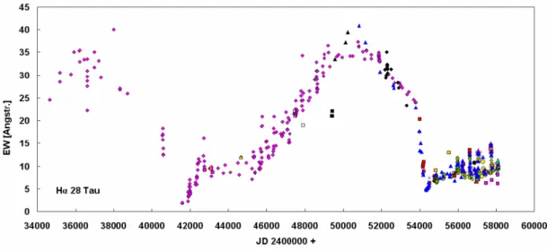
Capricorni (B3Ve). . . 43 1.22 Long-term variability of the H𝛼 equivalent width of 28 Tau (B8Vpe). . 44 1.23 Schemes of different dynamical models to form disks in Be stars. . . 47 1.24 Model intensity map (projected on the sky) in the K-band from Gies
et al. (2007) to the analysis of interferometric data of the Be star 𝛾 Cassiopeiae (B0.5IV). . . 53 1.25 Comparison of Be disks sizes derived in the H𝛼 line and in K-band from
the CHARA Array interferometric survey of Touhami et al. (2013). . . 54 1.26 Theoretical Be disk formation at different wavelength regions from
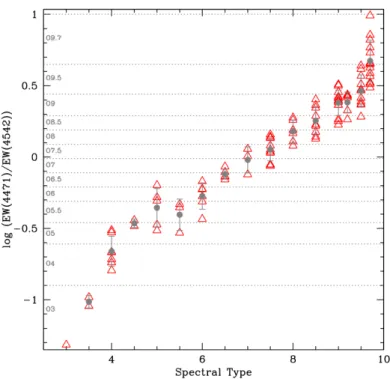
cal-culations with code HDUST. . . 55 2.1 Ratio between the equivalent width measured in He i 𝜆4471 and He ii
𝜆4542 as a function of spectral type of O stars (105 objects). . . 61 2.2 Visible spectra (∼4000-4700 Å) of O dwarfs (class V) from O9V to O2V. 62 2.3 Visible spectra (∼ 3800-4600 Å) from O9V to A0V stars, covering the
entire range of B dwarf stars (B0V-B9V). . . 63 2.4 Geometric scheme for the formation of P Cygni profiles. . . 66 2.5 Comparison of UV line formation through the wind extension. . . 67 2.6 CMFGEN ion fraction of silicon as a function of effective temperature
for the parameter space of O supergiant stars. . . 70 2.7 Effect of varying the effective temperature on the UV and visible regions. 71
2.8 Effect of varying the mass-loss rate on the UV (Si iv 𝜆𝜆 1394,1403), visible (H𝛼), and infrared (Pf𝛾 and Br𝛼) regions. . . 72 3.1 Schematic of an Airy disk, formed by the phenomenon of diffraction,
arising from the incidence of the light wavefronts into a telescope (round pupil). . . 76 3.2 Comparison between the angular resolution (in milliarcsecond) provided
by current single-mirror telescope (blue line ; ZIMPOL, IRDIS, VISIR instruments) and interferometric facilities (green line ; VEGA/CHARA, MATISSE, VLTI + CHARA instruments, and ALMA), as a function of wavelength. . . 77 3.3 Scheme for the propagation of light wavefronts through a double-slit
screen, the Young’s double-slit experiment. . . 79 3.4 Schematic representing the basic elements of an optical long-baseline
interferometer : the telescopes and optical subsystems (relay optics, delay line, and beam combination). . . 82 3.5 Simulated fringe patterns for objects of different sizes, observed using a
two-telescope interferometer. . . 83 3.6 Schematic of two different cases of spatial and temporal coherence. . . 84 3.7 Schematic of a triplet of telescopes used for measuring closure phase. . 89 3.8 Spectrally dispersed (∼2.156-2.175 𝜇m) fringes of 𝜂 Carinae measured
with VLTI/AMBER in high spectral resolution mode (HR, 𝑅 = 12000) at 26 February 2005. . . 92 3.9 Different scenarios for the kinematics of a circumstellar disk, calculated
using a kinematic model : purely-rotating disk, purely-expanding disk, and a hybrid case, respectively, from the left to the right panels. . . 94 3.10 Schematic layout of the CHARA Array, installed on the Mount Wilson
Observatory (California, USA). . . 96 3.11 Aerial view of the Very Large Telescope’s observing platform, installed
at the Cerro Paranal Observatory (Atacama desert, Chile). . . 98 3.12 Schematic layout of the VLTI Array. The Unit Telescopes (UT) are
indicated in red, fixed 8-m telescopes, with stations named from U1 to U4. 99 4.1 Schematic of a plane-parallel geometry. . . 104 4.2 Line-blanketing effect on the emergent spectrum. . . 112 4.3 Schematics of the (𝑝,𝑧) coordinate system, which is used in the code
CMFGEN to solve the radiative transfer problem (ray-by-ray solution method). . . 114
4.4 Intensity profiles, as a function of the wavelength (∼6530–6600 Å, around H𝛼), calculated by myself using CMFGEN . . . 115 4.5 Emergent flux (normalized to the continuum), computed from the same
CMFGEN model in Fig. 4.4, around the H𝛼 line (strong P Cygni profile).116 4.6 Distribution of the BeAtlas models with respect to the stellar mass and
base disk surface density. . . 119 4.7 First two rows : intensity maps (128 x 128 pixels) at different values
of wavelength close to Br𝛾 (from left to right : 2.161, 2.164, 2.165, and 2.166 𝜇) of two HDUST models, from the BeAtlas grid, with different values of inclination angle : 𝑖 = 0 (first row) and 𝑖 = 90° (second row). 123 5.1 Comparison between the visibility curves (squared visibility, 𝑉2) of two
uniform disks with different values of angular diameter : 𝜃UD = 0.1 mas
(black) and 1.0 mas (red). . . 126 5.2 Left panel : modeling to NPOI observations (interferometric data
cente-red on H𝛼) of the Be star 𝑜 Aquarii using geometric models. . . 127 5.3 Example of the graphical interface of LITpro, used in this case to model
VLTI/GRAVITY data of Rigel using a uniform disk model : best-fit model with angular diameter of ∼2.61 mas. See text for discussion. . . 129 5.4 Geometric modeling, using the software LITpro (Fig. 5.3), of our
VLTI/-GRAVITY data of Rigel : squared visibilities at the close-by continuum region (∼2.145-2.155 𝜇m) to Br𝛾. . . 130 5.5 Chart showing the calculation of the intensity map of the central star
plus disk system (total intensity map shown in the bottom) with the kinematic code. See text for discussion. . . 133 5.6 Comparison between kinematic models, calculated around the H𝛼 line,
by varying just one selected parameter : . . . 134 5.7 VLTI/AMBER observations in Br𝛾 (color lines) of the nova T Pyxidis at
different days since the outburst onset (28.76 days in orange and 35.77 days in green). . . 136 5.8 𝜒2 map to VEGA data of 𝑜 Aquarii for kinematic models (calculated
around H𝛼) with different values of disk size (major-axis FWHM of an elliptical Gaussian distribution, in stellar diameter). . . 137 5.9 Kinematic model disk size (in Br𝛾, fit to AMBER data of 𝑜 Aquarii)
sam-pled in a MCMC run using EMCEE with 300 walkers and 200 iterations in total. . . 140
6.1 Comparison between parametric HDUST models (𝑚 = 3.0, left panels) and steady-state non-isothermal HDUST models (non-parametric mo-dels, right panels). . . 213 7.1 VLTI/MATISSE observation of Rigel performed on September 25, 2019. 240 7.2 Intensity profiles from one of our adopted CMFGEN models for Rigel,
used as a reference model in our VLTI/GRAVITY proposal. . . 241 7.3 Simulated visibilities (left panel) and spectra (right panel) in the K-band
(GRAVITY wavelength region) from CMFGEN models with different values of mass-loss rate . . . 242 7.5 LITpro best-fit uniform disk models found from fitting our GRAVITY
data for Rigel, in the continuum region close to Br𝛾 (left panel) and in the core of Br𝛾 (right panel). . . 244 7.6 Image reconstruction by Chesneau et al. (2000) of P Cygni large-scale
cir-cumstellar environment (up to ∼1000 𝑅⋆) using Observatoire de Haute-Provence (OHP) observations with adaptive optics. . . 245 7.7 SPHERE simulated observations (raw images) from our reference
CMF-GEN model for Rigel (with mass-loss rate of 4 × 10⁻⁷ M
⊙yr−1). . . 246
7.8 Example of AMBER differential data (red line) of 𝛼 Arae observed in the Be survey of Meilland et al. (2012). . . 247 7.9 Left : example of H𝛼 line profiles observed with the VEGA instrument
for 17 Be stars of our VEGA survey (34 objects observed in total). . . . 248 7.10 Observation of the Be star 𝛼 Arae with VLTI/MATISSE from the L-band
to the M-band (covering ∼3.0-5.0 𝜇m). . . 249 7.11 Preliminary MCMC analysis of VLTI/MATISSE differential data (in the
Br𝛼 line) of the Be star 𝛼 Arae . . . 250 7.12 Geometric modeling of VEGA squared visibilities of the late-type Be
1.1 Summary of the stellar parameters of OB-type dwarfs (luminosity class V) from spectral type calibrations in the literature. Parameters for B stars are from Townsend et al. (2004) and O stars from Martins et al. (2005a). . . 3 2.1 Summary of the main ultraviolet, visible, and infrared line diagnostic used
to determine the photospheric and wind parameters of massive stars, in particular, O-type, WR, and B supergiant stars. Adapted from Martins (2011). . . 69 3.1 Summary of some very first visible and infrared interferometric studies
using two-telescope configuration. Reproduced from Léna (2014). . . . 80 3.2 Summary of telescope arrays with spectro-interferometric instruments.
Adapted from Hadjara (2017). . . 95 4.1 Summary of basic characteristics of non-LTE and line-blanketed radiative
transfer codes for modeling massive hot stars. Adapted from Chap. 5 of Crivellari et al. (2019) . . . 109 4.2 List of HDUST parameter in the BeAtlas grid. The first row indicates
the spectral type corresponding to the stellar mass for B dwarfs (Town-send et al. 2004). All the model are calculated with the following fixed parameters : scale height at the disk base 𝐻0 = 0.72, fraction of H in
the core 𝑋𝑐 = 0.30, metallicity 𝑍 = 0.014, and disk radius = 50 𝑅eq.
1 Introduction 1
1.1 OB-type stars . . . 2
1.1.1 Physical properties and stellar evolution . . . 2
1.1.2 Enrichment of the interstellar medium . . . 6
1.2 Radiative line-driven winds . . . 11
1.2.1 The phenomenon of stellar winds . . . 11
1.2.2 Elementary concepts of radiative line-driven winds . . . 13
1.2.3 Radiative winds in the HR diagram . . . 25
1.3 Stellar rotation . . . 29
1.3.1 Effects on the stellar shape . . . 29
1.3.2 Stellar rotational rate and oblateness . . . 31
1.3.3 The von Zeipel effect . . . 33
1.3.4 Fast rotation . . . 35
1.4 The Be phenomenon . . . 40
1.4.1 Characterization and physical origin . . . 40
1.4.2 Variability in Be stars . . . 42
1.4.3 Oe and Ae stars : counterparts to the Be phenomenon ? . . . 45
1.5 Circumstellar disks of Be stars . . . 46
1.5.1 Formation and dynamics . . . 46
1.5.2 Geometry and size . . . 52
2 Stellar spectroscopy 58
2.1 Stellar classification . . . 58
2.2 Line formation in the wind : P-Cygni profiles . . . 64
2.3 Multi-wavelength line diagnostics . . . 68
3 Optical long-baseline stellar interferometry 74 3.1 Why we need high angular resolution observations ? . . . 74
3.2 Historical overview . . . 78
3.3 Elementary concepts of OLBI . . . 81
3.4 Light coherence . . . 85
3.5 Interferometric quantities . . . 87
3.5.1 The Zernike-van Cittert theorem . . . 87
3.5.2 Closure phase . . . 89
3.5.3 Visibility calibration . . . 90
3.6 Spectro-interferometry . . . 91
3.7 Spectro-interferometric instruments . . . 95
3.7.1 The CHARA array . . . 95
3.7.2 CHARA/VEGA . . . 97
3.7.3 The VLTI array . . . 97
3.7.4 VLTI/AMBER . . . 100
3.7.5 Comparison between CHARA and VLTI . . . 100
4 Radiative transfer modeling 102 4.1 Elementary concepts of radiative transfer . . . 102
4.2 Overview on radiative transfer codes for hot stars . . . 108
4.3 The code CMFGEN . . . 110
4.4 The code HDUST and the BeAtlas grid . . . 116
4.5 For what CMFGEN and HDUST are suited ? . . . 120
5 Model fitting of interferometric data 124
5.1 Geometric models . . . 125
5.1.1 Applying the Zernike-van Cittert theorem to analytical models . 125 5.1.2 The simplest case : an example of one-component model . . . . 125
5.1.3 Adding other components : an example of two-component model 126 5.2 Analytical model fitting : the software LITpro . . . 128
5.2.1 Overview : a tool dedicated to interferometric modeling . . . 128
5.2.2 Example of modeling : VLTI/GRAVITY data of Rigel . . . 129
5.2.3 Limitations : what is the global 𝜒2 minimum ? . . . 130
5.3 The kinematic code . . . 131
5.3.1 Overview : the model parameters . . . 131
5.3.2 Model description : the central star and the circumstellar envi-ronment . . . 132
5.3.3 Parameters effects on the interferometric quantities . . . 134
5.3.4 An example of model fitting : AMBER data of the nova T Pyxidis135 5.4 Kinematic model fitting using MCMC . . . 136
5.4.1 Why use a MCMC fitting-method to the kinematic code ? . . . 136
5.4.2 The MCMC method . . . 138
5.4.3 The code EMCEE : a MCMC implementation . . . 138
5.4.4 Using prior information with EMCEE . . . 139
5.4.5 Example of modeling : VLTI/AMBER data of 𝑜 Aquarii . . . . 139
5.4.6 Further improvements . . . 141
6 Published studies 142 6.1 Mini-survey of O stars . . . 143
6.1.1 Problems with the theory of line-driven winds : weak winds . . . 143
6.1.2 Master thesis work . . . 144
6.1.3 Improvements during my PhD . . . 145
6.2 The LBV star P Cygni . . . 194
6.2.1 Winds and episodic outbursts of LBVs . . . 194
6.2.2 Intensity interferometry in a nutshell . . . 195
6.2.3 My collaboration with the I2C team . . . 195
6.2.4 Results and conclusions . . . 196
6.3 The Be-shell star 𝑜 Aquarii . . . 208
6.3.1 Probing the Be phenomenon : why study 𝑜 Aquarii with interfe-rometry ? . . . 208
6.3.2 Observing 𝑜 Aquarii in the AMBER and VEGA Be surveys . . . 209
6.3.3 A multi-technique modeling approach : from analytical to nume-rical models . . . 210
6.3.4 Results and conclusions . . . 211
7 Ongoing studies 238 7.1 The radiative line-driven wind of Rigel . . . 238
7.1.1 Rigel : an evolved massive star . . . 238
7.1.2 Multi-band spectro-interferometry : CHARA and VLTI . . . 239
7.1.3 H𝛼 intensity interferometry : I2C team . . . 243
7.1.4 Direct imaging : VLT/SPHERE . . . 245
7.2 Classical Be stars . . . 246
7.2.1 Drawing a big picture of Be disks . . . 246
7.2.2 The VEGA and AMBER large surveys . . . 247
7.2.3 First observations with MATISSE . . . 249
7.2.4 Toward a detailed view on Be stars (other than 𝑜 Aquarii) . . . 251
8 Conclusions and perspectives 253
Introduction
Contents
1.1 OB-type stars . . . . 2
1.1.1 Physical properties and stellar evolution . . . 2
1.1.2 Enrichment of the interstellar medium . . . 6
1.2 Radiative line-driven winds . . . . 11
1.2.1 The phenomenon of stellar winds . . . 11
1.2.2 Elementary concepts of radiative line-driven winds . . . 13
1.2.3 Radiative winds in the HR diagram . . . 25
1.3 Stellar rotation . . . . 29
1.3.1 Effects on the stellar shape . . . 29
1.3.2 Stellar rotational rate and oblateness . . . 31
1.3.3 The von Zeipel effect . . . 33
1.3.4 Fast rotation . . . 35
1.4 The Be phenomenon . . . . 40
1.4.1 Characterization and physical origin . . . 40
1.4.2 Variability in Be stars . . . 42
1.4.3 Oe and Ae stars: counterparts to the Be phenomenon? . . . . 45
1.5 Circumstellar disks of Be stars . . . . 46
1.5.1 Formation and dynamics . . . 46
1.5.2 Geometry and size . . . 52
Stars are unique astrophysical objects to test our understanding about the basic structure of nature. For example, observations of solar neutrinos provided the first clear evidence of the quantum phenomenon called neutrino oscillation, implying that at least one of the neutrino flavors has non-zero mass (e.g., see the Nobel Lecture of McDonald 2016). This disagrees with the so-called Standard Model of elementary particles, and thus opens an entire branch of theoretical research of physics beyond the Standard Model. Conversely, apart from the current understanding of star formation, the study of stars is very well-founded in terms of fundamental physics: combining the background from hydrodynamics, thermodynamics and statistical physics, atomic and molecular physics, and electromagnetism, among others.
The aim of this thesis is to analyse the physical properties and mass loss processes of massive hot stars and study their close environments, ranging from radiatively driven winds (with velocities up to a thousand km s-1) to quasi-stable thin equatorial disks
in rotation. For this purpose, different observational techniques and also modeling methods are employed in this work. In this chapter, I overview in details the current understanding about OB-type stars.
1.1
OB-type stars
1.1.1
Physical properties and stellar evolution
O-type stars (MZAMS1& 17 M⊙) are subject to extreme physical conditions, showing
the highest value of luminosity and effective temperature (𝑇eff) among the canonical
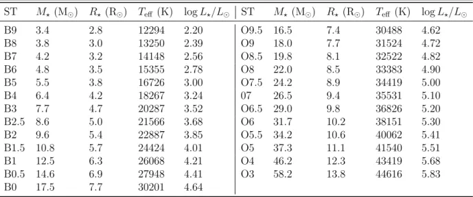
Table 1.1 – Summary of the stellar parameters of OB-type dwarfs (luminosity class V) from spectral type calibrations in the literature. Parameters for B stars are from Townsend et al. (2004) and O stars from Martins et al. (2005a).
ST 𝑀⋆(M⊙) 𝑅⋆ (R⊙) 𝑇eff (K) log 𝐿⋆/𝐿⊙ ST 𝑀⋆ (M⊙) 𝑅⋆(R⊙) 𝑇eff (K) log 𝐿⋆/𝐿⊙
B9 3.4 2.8 12294 2.20 O9.5 16.5 7.4 30488 4.62 B8 3.8 3.0 13250 2.39 O9 18.0 7.7 31524 4.72 B7 4.2 3.2 14148 2.56 O8.5 19.8 8.1 32522 4.82 B6 4.8 3.5 15355 2.78 O8 22.0 8.5 33383 4.90 B5 5.5 3.8 16726 3.00 O7.5 24.2 8.9 34419 5.00 B4 6.4 4.2 18267 3.24 07 26.5 9.4 35531 5.10 B3 7.7 4.7 20287 3.52 O6.5 29.0 9.8 36826 5.20 B2.5 8.6 5.0 21566 3.68 O6 31.7 10.2 38151 5.30 B2 9.6 5.4 22887 3.85 O5.5 34.2 10.6 40062 5.41 B1.5 10.8 5.7 24424 4.01 O5 37.3 11.1 41540 5.51 B1 12.5 6.3 26068 4.21 O4 46.2 12.3 43419 5.68 B0.5 14.6 6.9 27948 4.41 O3 58.2 13.8 44616 5.83 B0 17.5 7.7 30201 4.64
Morgan-Keenan system of stellar classification (Morgan et al. 1943). Based on sophis-ticated spectral type calibrations (Martins et al. 2005a), a typical late-type O dwarf (O9.5V) has 𝑇eff ∼ 30500 K and bolometric luminosity 𝐿⋆ ∼ 41700 L⊙. On the other
hand, an earlier and also (supposedly) more evolved O star is expected to have a quite higher effective temperature and luminosity: 𝑇eff ∼ 42600 K and 𝐿⋆ ∼ 1000000 𝐿⊙
(e.g., O3I).
With lower effective temperature, B-type dwarfs encompass both the range of intermediate- and high-mass stars, having MZAMS between ∼3 M⊙ (B9V, 𝑇eff ∼12000
K) and ∼18 M⊙ (B0V, 𝑇eff ∼ 30000 K). The physical parameters of OB-type dwarf
stars are summarized in Table 1.12. Thus, mainly depending on their initial mass,
B dwarfs are progenitors of either planetary nebulae (MZAMS . 8-9 M⊙), resulting in
white dwarfs as stellar remnant, or core-collapse supernovae that result in neutron stars from the more massive progenitors (e.g., see Fig. 1 of Heger et al. 2003).
Despite being much more abundant than massive stars, based on a typical Salpeter initial mass function (Salpeter 1955), low- and intermediate-mass stars (MZAMS . 8
M⊙) are only able to carry the stellar nucleosynthesis up to the core helium-burning
phase, resulting in the production of carbon and oxygen during their more evolved phases as asymptotic giant branch (AGB) stars. From Table 1.1, one sees that this applies to B stars among the types B9 and B3. However, massive stars (MZAMS & 8
M⊙) are able to continue the nucleosynthesis in their cores beyond the helium-burning
phase up to the production of iron group elements during the silicon-burning phase,
2. In Table 1.1, the quoted value for the initial mass of a B0 dwarf is somewhat larger than for an O9.5 dwarf. We emphasize that this fact is not physically reliable and it happens since the results complied in this table come from different studies in the literature.
Figure 1.1 – Schemes of chemical stratification in evolved massive stars (left) and evolved low-intermediate-mass (right) stars. Left: reproduced from Maeder (2009). Right: reproduced from Herwig (2005).
resulting in core-collapse supernovae (type II, Ib, or Ic).
Fig. 1.1 presents a basic scheme of the chemical stratification in the structure of evolved massive stars, as well as of evolved low-intermediate-mass stars (AGB phase). One sees that concentric layers are successively composed by lighter elements (as H and He) toward the stellar surface. We stress that this description for the fate of stars according to the initial mass is a simplified picture. For instance, it is still largely unknown the pathways of stars with initial masses between ∼8-10 M⊙. In this case,
depending on the mass loss, they can either evolve to the AGB phase, ending their evolution as planetary nebulae, or evolve up to core-collapse supernovae (e.g., Nomoto 1984, 1987; Jones et al. 2013).
The evolution of massive stars results in different types of supernovae, depending mainly on the initial stellar mass and metallicity (e.g., see Fig. 2 of Heger et al. 2003). In Fig. 1.2, we show the modified Conti scenario for the evolution of single non-rotating stars with solar-metallicity, as a function only of their initial masses (Ekström et al. 2013). This is inspired on the scenario originally proposed by Conti (1975), the first study to propose the evolutionary connection between O-type and Wolf-Rayet stars. Nevertheless, this scheme, presented in Fig. 1.2, is a summary of modern results found by state-of-the-art evolutionary models for massive stars calculated using the Geneva stellar evolution code (Ekström et al. 2012).
From Fig. 1.2, we see that stars with MZAMS lower than about 30 M⊙ will end
their evolution as red supergiants (𝑇eff up to ∼ 4000 K, Levesque et al. 2005), before
exploding in type-II supernovae (hydrogen-rich core-collapse supernovae). On the other hand, massive stars with MZAMS larger than 30 M⊙ will finish their evolution as
Wolf-Figure 1.2 – Modified Conti scenario for the evolutionary scheme of massive stars as a function of zero-age main sequence mass. Reproduced from Ekström et al. (2013).
Rayet stars (𝑇eff up to ∼ 200000 K, Tramper et al. 2015), before exploding in type-Ib
or type-Ic supernovae (hydrogen-deficient core-collapse supernovae). It is interesting to note that stars with initial masses between 30 and 40 M⊙ are expected to loop between
the two extreme regions of the HR diagram, passing from the blue to the red supergiant phases and then returning to the blue region of the HR diagram as Wolf-Rayet stars. As pointed out by Ekström et al. (2013), for these more massive stars that can evolve to red supergiants, stellar winds during this phase must be intense enough, in comparison with stars with 10 M⊙ < MZAMS < 30 M⊙, to remove the hydrogen from their atmospheres
and thus resulting in Wolf-Rayet stars, which show very weak or absent hydrogen lines in their spectra.
We stress that the scheme shown above is based on non-rotating models for single stars with solar-metallicity. Other relevant physical processes, which are not taken into account here, must affect these results: metallicity, rotation, magnetic fields, tidal interaction and mass transfer in binary systems, and more accurate values for the wind mass-loss rate at different evolutionary stages. For instance, it is known that a large fraction (up to ∼70%) of massive stars are born in multiple system and a significant fraction (up to ∼30%) of the current single massive stars are in fact merger products from binary system formed in the past (e.g., Sana et al. 2012, 2013a; de Mink et al. 2014). A more detailed discussion on the effects of magnetic field, rotation, and multiplicity, on the evolution of massive stars can be found in Meynet et al. (2011), Meynet et al. (2015), and Sana et al. (2013c), respectively.
In short, our discussion above evidences the importance of mass loss processes on the properties and evolution of massive stars. In particular, Sect. 1.2 is devoted to discuss in details the phenomenon of stellar winds.
As a quantitative example, we show, in Fig. 1.3, how the mass-loss rate of the stellar wind is expected to change as a function of time for a non-rotating single star with MZAMS = 60 M⊙. These values for the mass-loss rate are taken in account in the
Geneva models analysed in Groh et al. (2014). Based on synthetic spectra (calculated with the radiative transfer code CMFGEN) at each evolutionary step, they studied
Figure 1.3 – Mass-loss rate (left axis, solid line) and stellar mass (right axis, dashed line) as function of age in the Geneva evolutionary model for a non-rotating single star with MZAMS = 60 M⊙. Colors
encode different evolutionary phases: H-core (blue), H-shell and H+He-shell (gray), and He-core (orange). The evolution of the spectral type predicted by Groh et al. (2014) is also indicated here. Due to the large amount of mass loss since the beginning of the main sequence, the star ends its evolution with about 13 M⊙. Adapted from Groh et al. (2014).
the spectroscopic properties of a non-rotating single 60 M⊙ star, evaluating how the
spectra type changes as the modeled star evolves from the H-burning phase to the pre-supernova phase.
Interestingly, Groh et al. (2014) showed that a single non-rotating star with MZAMS
= 60 M⊙ must appear in the zero-age main sequence as a O3-4 supergiant (luminosity
class I), not as a dwarf star (class V). After that, the star evolves to the LBV and Wolf-Rayet phases before ending its evolution. From Fig. 1.3 one sees that the mass-loss rate changes highly through the evolution, from ∼10−6 M
⊙ yr-1at the beginning of the
H-core burning phase, reaching a maximum of ∼10−3 M
⊙ yr-1 by the end of the cool
LBV phase. Due to the mass loss, this star with an initial mass of 60 M⊙ will end its
evolution with about 13 M⊙, as a WO1 star until the supernova explosion (Groh et al.
2014).
1.1.2
Enrichment of the interstellar medium
Stars transfer mechanical and radiative energy to the interstellar medium (ISM) by different ways: stellar winds (in addition to episodic mass loss), radiation, and super-novae. In Fig. 1.4, we show the central part of the H ii region 30 Doradus (Tarantula Nebula), called R136, in the Large Magellanic Cloud. This region has been widely stud-ied regarding very massive stars (MZAMS ≈ 100-300 M⊙) and multiplicity properties
Figure 1.4 – The R136 open cluster located in the H ii region 30 Doradus (Tarantula Nebula) in the Large Magellanic Cloud. Imaging from the Hubble Space Telescope/Wide Field Camera instrument in the visible region (photometry in the U-, B-, V-, I-, and H𝛼-bands). This image has field of view of about 46 pc. Source: https://apod.nasa.gov/apod/ap160124.html.
From that, we note that R136 is a very crowded stellar environment. In fact, it is the region of highest stellar density in Tarantula Nebula, being populated by a large number of OB-type stars. The spectroscopic analysis of Doran et al. (2013) confirmed about 500 early-type stars in this region. Massive hot stars are the main source of ultraviolet (UV) radiation, ionizing the nebular gas, remnant of the primordial molecular cloud, and then originating H ii regions. Moreover, we see that the structure of 30 Doradus is highly shaped due to the interaction of the intense winds and radiation fields from early-type stars with the ISM gas.
Therefore, it is conspicuous the importance of massive stars in the enrichment of the ISM, both from a physical (transfer of kinematic energy) and chemical (production and transfer of metals) views. Abbott (1982a) was one of the first quantitative studies to investigate the effects of the winds of massive stars on the ISM. This author evaluated the mechanical and radiative energy contribution from O-type, BA supergiants, and Wolf-Rayet stars to the enrichment of the ISM within a distance of ∼3 kpc. He found that these stars transfer mass (by means of winds) and radiation to the ISM at a rate of 9 × 10⁻⁵ M
⊙ yr-1 kpc-2 and 2 × 1038 erg s-1 kpc-1, respectively.
Fig. 1.5 shows the results found by Castor (1993) for the rate of mass that is injected into the interstellar medium as a function of initial stellar mass. This rate (in units of M yr-1 kpc-2) is weighted by the initial mass function from Garmany et al. (1982).
Figure 1.5 – Mass return rate (logarithmic scale) of massive stars as a function of stellar mass. The evolutionary phases are indicated at the different regions here: O-type, BA supergiant, luminous blue variable (LBV), red supergiant (RSG), carbon Wolf-Rayet (WC), and nitrogen Wolf-Rayet (WN) stars. The region of core-collapse supernovae is indicated by SN. The stellar mass is shown in logarithmic scale. Apart from the stellar mass that returns to the interstellar medium due to supernovae, the peak of mass return comes from stars with initial mass of about 40 M⊙ during the Wolf-Rayet phase.
Reproduced from Lamers & Cassinelli (1999).
In short, it expresses the contribution to the enrichment of the ISM given the initial mass through the different evolutionary phases of massive stars. First, notice that stars with MZAMS ∼ 8-10 M⊙ will transfer mass to the ISM mainly at the end of their
evolutionary paths, when exploding in core-collapse supernovae of type-II (Fig. 1.2). Despite having less intense winds than the more massive stars, these stars with MZAMS
∼8-10 M⊙ also significantly contribute to the mass return to the ISM, taking the SN
contribution into account, since they are more numerous in comparison with the more massive objects. Apart from the mass injection by means of supernovae, the largest individual contribution to the enrichment of the ISM comes from stars with initial masses of ∼40 M⊙ during their evolutionary stages as Wolf-Rayet stars.
However, as pointed out in Sect. 1.1.1, B dwarfs encompasses both intermediate-mass (MZAMS of ∼ 3 M⊙, type B9) and high-mass stars (MZAMS of ∼ 18 M⊙, type B0).
These lower-mass B stars will then evolve to the AGB phase. Our discussion above was focused on the contribution of massive stars to the enrichment of the ISM, but AGB stars are also important contributors of gas and dust to the ISM by their intense winds. Due to winds, mainly during the AGB phase, a star with MZAMS of ∼ 4 M⊙ is expected
Figure 1.6 – Amount of dust mass produced by AGB stars and supernovae as a function of progenitor initial mass from Gall et al. (2011b). The theoretical curve for AGB stars is shown in green, while the curves for supernovae are shown in blue, pink, and cyan according to the dust production efficiency that is used in the models. Measured values for supernovae remnants are shown in colored points according to different values of dust temperature. Further details on these theoretical curves and measured values are found in Sect. 7.2 of Gall et al. (2011b). See text for discussion. Reproduced from Gall et al. (2011b).
to loose about 80% of its initial mass (e.g., Cummings et al. 2016).
AGB stars are responsible to about the half of the recycled gas that is used in the star formation process (e.g., Maeder 1992), and they are important sources of dust in the Universe (see, e.g., Valiante et al. 2009; Gall et al. 2011b, and references therein). Fig. 1.6 shows the predictions from Gall et al. (2011b) for the amount of dust yield both by AGB stars and supernovae. These theoretical curves are compared with measured values for supernovae remnants from the literature. Here, the theoretical curves for supernovae are calculated considering different regimes of dust production efficiency, which is related to the total amount of dust injected into the ISM (see Eq. 21 of Gall et al. 2011a). From that, one sees that the amount of dust produced by AGB stars is somewhat comparable to the one by supernovae regardless of the different theoretical scenarios that are analysed by these authors.
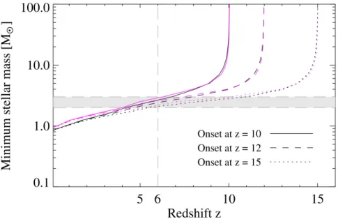
In addition, Fig. 1.7 shows the minimum initial stellar mass for a star dying at a certain epoch (expressed in terms of cosmological redshift 𝑧). Considering the onset of star formation at 𝑧 = 10, just very massive stars with mass up to ∼100 M are able to
Figure 1.7 – Minimum MZAMSthat allows a complete stellar evolution at a certain value of cosmological
redshift (𝑧). Stellar formation starts on three different value of redshift: 𝑧 = 10 (solid line), 𝑧 = 12 (dashed line), and 𝑧 = 15 (dotted line). Black lines corresponds to stellar metallicity 𝑍 = 0.001 and pink lines to 𝑍 = 0.040. The gray region indicates the minimum initial mass (∼2-3 M⊙) for stars
contributing (in this case, during the AGB phase) to the injection of dust into the ISM in the early Universe (𝑧 = 6). Reproduced from Gall et al. (2011b).
contribute to the enrichment of the ISM at this epoch (Gall et al. 2011b).
Based on Fig. 1.7, we see that only stars with MZAMS larger than ∼3 M⊙ are able
to pollute the ISM at the epoch 𝑧 = 6 (Universe with age of ∼ 109 yr). Stars with
initial mass lower than this threshold evolve in time-scales longer than the age of the Universe at 𝑧 = 6. In short, OB-type dwarfs are the progenitors of the sources of the ISM gas and dust at the early Universe.
In conclusion, massive star are rare due to the initial mass function and also to their shorter lifetimes of ∼106-108 Myr. As a rough estimate, there are only ∼14000-18000
O-type stars in the Galaxy (Maíz Apellániz et al. 2013). Despite their rarity, these stars are important because they enrich physically and chemically the ISM with their strong outflows, since the beginning of the main sequence until evolved stages as BSG, RSG, LBV, and Wolf-Rayet stars. Moreover, they are progenitors of more exotic astrophysical objects, neutron stars and black holes, that are connected to high-energy astrophysical phenomena, as gamma-ray bursts and gravitational waves (e.g., Gehrels & Razzaque 2013; Abbott et al. 2016).
1.2
Radiative line-driven winds
1.2.1
The phenomenon of stellar winds
Stellar winds are characterized by a continuous process of mass loss from the stellar atmosphere (i.e., the photosphere3). The reader should pay attention here to the
property of continuity because massive stars lose mass by means of other mechanisms during their evolution, such as supernovae or episodic mass eruptions that eject a large amount of matter in a limited amount of time (time-scale of years), as the giant mass loss eruption that occurred at P Cygni (LBV star, spectral type B1-2Ia) in the 17th century (see, e.g., Israelian & de Groot 1999; Smith 2014).
The mass-loss rate ( ˙𝑀) and the terminal velocity (𝑣∞) are the main fundamental
parameters to describe the hydrodynamics of the wind. With respect to a larger astro-physical context, it is important to constrain the real values for these two parameters in massive stars because they directly provide the kinematic energy injected into the interstellar medium through winds by the wind power 𝑃𝑊 (Abbott 1982a):
𝑃𝑊 =
1
2𝑀 𝑣˙ ∞2. (1.1)
The mass-loss rate is defined as the quantity of mass that the star loses via winds per unit time:
˙
𝑀 = −𝑑𝑀⋆
𝑑𝑡 , (1.2)
where 𝑀⋆ is the stellar mass (expressed as a function of time).
The terminal velocity is the wind velocity that is reached at a sufficiently large distance from the stellar surface (𝑟 → ∞) for enabling null-acceleration (as a result of null-force) on the wind.
These two basic parameters of the wind, ˙𝑀 and 𝑣∞, are related to each one by the
equation of mass continuity:
˙
𝑀 = 4𝜋𝑟2𝜌(𝑟)𝑣(𝑟), (1.3)
where 𝜌(𝑟) is the wind density structure and 𝑣(𝑟) is the wind velocity structure for a certain distance 𝑟 from the center of the star (𝑟 ≥ 𝑅⋆).
Eq. 1.3 stands in the case of a stationary (i.e., time-independent, 𝜕𝑣(𝑟,𝑡)
𝜕𝑡 = 0), smooth, and spherically symmetrical wind. It expresses the conservation of mass through the wind, that is, the same quantity of mass (gas) flows, per unit time, through
3. Throughout this thesis, the terms “(stellar) atmosphere” and “extended atmosphere” are occa-sionally used to design the photosphere and the circumstellar environment, respectively.
a sphere with area given by 4𝜋𝑟2 (at any value of 𝑟).
Based on solutions for the momentum equation of the wind from Castor et al. (1975), the wind velocity structure, 𝑣(𝑟), is usually parameterized in the literature by
the so-called 𝛽-law approximation:
𝑣(𝑟) = 𝑣0+ (𝑣∞− 𝑣0) (︃ 1 −𝑅⋆ 𝑟 )︃𝛽 , (1.4)
where 𝑅⋆ is the stellar radius, 𝑣0 is the velocity at the photosphere (i.e., the base of the
wind is set at the photosphere), and 𝑟 is given as a function of 𝑅⋆. Considering that
𝑣∞>> 𝑣0, Eq. 1.4 can be approximated as follows:
𝑣(𝑟) = 𝑣∞ (︃ 1 − 𝑅⋆ 𝑟 )︃𝛽 . (1.5)
Thus, given the terminal velocity 𝑣∞, the wind velocity is fully parameterized by
the exponent 𝛽. Based on spectroscopic and hydrodynamical studies, 𝛽 is typically found around 0.8-1.0 for O dwarfs (luminosity class V) stars (e.g., Bouret et al. 2013; Muijres et al. 2012). On the other hand, 𝛽 can reach larger values up to ∼ 2.0-3.0 in OB supergiants (e.g., Crowther et al. 2006; Martins et al. 2015). From Eq. 1.5, we note that higher values of 𝛽 implies that the wind accelerates slower. Curé & Rial (2004) investigated the effect of rotation on the wind acceleration of massive stars, and they verified that solutions for slow velocity winds are acceptable in the case of fast rotators, having rotational velocities higher than about 75% the critical value (Sect. 1.3.2). This could be in part one possibility to explain such large values of 𝛽 that are typically observed in more evolved massive stars.
We point out that winds are common in different types of stars: both in young and evolved low-mass stars (e.g., T-Tauri, solar-type, and AGB stars) and in young and evolved massive stars. Despite being created by different physical mechanisms, this means that winds happens virtually in all types of stars, having different effects on stellar evolution depending on the intensity of the mass-loss rate.
For instance, the Sun shows a stable outflow that is well characterized by a quiescent mass-loss rate of ∼10−14 M
⊙ yr-1and a terminal velocity of ≈ 400 km s-1(e.g., Sturrock
et al. 1986). The solar wind is driven by gas pressure due to the high temperature of the solar corona (e.g., Noble & Scarf 1963). Parker (1958) was the first to show quantitatively that a static solar corona is impossible, introducing the term “stellar wind”. Further details on coronal winds can be found in Chapter 5 of Lamers & Cassinelli (1999). For a better comparison with these values mentioned for the Sun, O-type stars
show mass-loss rates up to ∼10−6 M
⊙ yr-1 and terminal velocities up to ≈3000 km s-1
in winds of solar-type stars during the main sequence.
More generally, intermediate- and low-mass stars develop winds with higher mass-loss rates just during evolved (more luminous) evolutionary phases, such as the AGB phase. In this case, mass-loss rates vary from ∼10−7 M
⊙ yr-1 at the initial AGB phase
up to ∼10−4 M
⊙ yr-1 at the end of the AGB phase. This later and more intense wind
phase is called as the AGB super-wind phase (Renzini 1981; Bowen & Willson 1991). It is thought that such very slow winds (𝑣∞ up to ∼30 km s-1) showing a large amount
of mass loss are driven during the AGB phase as follows (e.g., Höfner & Andersen 2007): pulsations transfer gas from the stellar surface to the outer atmospheric layers, where the temperature is low enough to enable the formation of dust grains. From that, the radiative pressure on the coupled system of gas and dust grains (carbonaceous or silicates) drives a steady outflow. The reader interested on further details regarding the mass loss of AGB stars is refereed to the review of Höfner & Olofsson (2018).
In short, intermediate- and low-mass stars are important to the enrichment of the interstellar medium, as discussed in Sect. 1.1.2, but this contribution is limited to later evolutionary phases. Their contribution is also limited in terms of heavy elements: they will mostly enrich the ISM with the injection of carbon, nitrogen, and oxygen. On the other hand, winds of massive stars are relevant during all their evolutionary phases, since the main sequence phase up to their later stages. Due to their high effective temperatures and luminosities, up to ∼106 times the solar luminosity, OB-type stars
are able to develop radiative line-driven winds, as discussed below.
1.2.2
Elementary concepts of radiative line-driven winds
Radiative line-driven winds means that the wind acceleration arises from the scat-tering of the stellar continuum flux by line transitions of (mainly) elements heavier than hydrogen and helium, creating spectral absorption and emission lines. Such photon-matter interaction transfers linear momentum from the stellar radiation field to the gas that composes the photosphere and the wind, and thus dropping the assumption of hydrostatic equilibrium for the stellar atmosphere.This mechanism for driving winds is not limited to massive hot stars, such as OB dwarfs, OBA supergiants, LBVs, and WR stars. After the post-AGB phase, low-and intermediate-mass stars will develop radiative-line driven winds during the phase as central stars of planetary nebula (CSPN) (e.g., Cerruti-Sola & Perinotto 1985; Prinja 1990). Despite having quite low luminosities, when compared with massive stars, CSPNs show very high effective temperature, reaching extreme values as high as ∼150000 K (e.g., Herald & Bianchi 2011; Keller et al. 2011). Moreover, the line-driven mechanism is promising to explain the origin of winds in the accretion disks of
quasars (e.g., Shlosman et al. 1985; Proga et al. 2000). Concerning the massive stars with low 𝑇eff, as the RSGs, the mechanisms for the wind acceleration are thought to
be quite similar to the ones described for AGBs stars in Sect. 1.2.1: a combination of stellar pulsations and radiative pressure on the coupled system of gas and dust grains (that are formed in outer atmospheric layers).
Considering the simplest case of stationary winds, and that the only forces exerted are due the gravity, the gas pressure gradient, and the radiation, the momentum equation of a radiation line-driven wind is expressed as follows:
𝑣d𝑣 d𝑟 = − 𝐺𝑀⋆ 𝑟2 + 1 𝜌 d𝑝(𝑟) d𝑟 + 𝑔rad(𝑟), (1.6)
where 𝐺 is the gravitational constant, 𝑀⋆ is the stellar mass, and 𝑝 is the gas pressure.
Assuming the case of a ideal gas with isothermal temperature 𝑇 , the state equation is described by:
𝑝(𝑟) = 𝑅𝑇
𝜇 𝜌(𝑟), (1.7)
where √︁𝑅𝑇
𝜇 is the isothermal sound speed in the wind, 𝑅 is the ideal gas constant
and 𝜇 is the mean molecular weight of the gas (𝜇 = 0.602 for an atmosphere with solar-metallicity).
On the right hand of Eq. 1.6, the first two terms are common when describing the hydrodynamics of different types of stellar winds. However, the third-term in the equation of motion represents the total radiative acceleration acting on the wind and is expressed as follows:
𝑔rad(𝑟) = 𝑔𝑒(𝑟) + 𝑔line(𝑟), (1.8)
since this results from the momentum transfer by two different ways of photon-atom interaction:
(i) 𝑔𝑒 is the radiative acceleration due to Thomson scattering (i.e., elastic scattering
of photons by electrons, the contribution from the continuum opacity). (ii) 𝑔line is the contribution due to line opacity (bound-bound transitions).
In addition, free-free and bound-free transitions also contribute to the radiative force due to continuum opacity (see, e.g., Eq. 26 of Sander et al. 2015).
Note that both terms are explicitly written here as a function of 𝑟. The first term in Eq. 1.8 is given by:
𝑔𝑒(𝑟) =
𝜅𝑒𝐿⋆
where 𝜅𝑒 is the opacity for electron scattering, 𝐿⋆ is the stellar luminosity, and 𝑐 is
the light speed in the vacuum. The term 𝜅𝑒 is dependent on the gas metallicity and
also the degree of gas ionization that typically ranges from ∼0.28 to 0.35 cm2g−1 in
early-type stars.
From Eq. 1.9, the Eddington parameter Γ𝑒 is defined as the ratio between the
radiative acceleration contribution from Eq. 1.9 and the gravitational acceleration 𝑔(𝑟), which is given by 𝐺𝑀⋆/𝑟2: Γ𝑒= 𝑔𝑒(𝑟) 𝑔(𝑟) = 𝜅𝑒𝐿⋆ 4𝜋𝐺𝑀⋆𝑐 , (1.10)
where 𝑀⋆ is the stellar mass.
Physically, this parameter expresses how close a star is to the gravitationally un-bound limit (Γ𝑒 → 1, the so-called classical Eddington limit), just considering the
radiative force due to electron scattering. From that, most massive hot stars have Γ𝑒
up to a factor of 2 lower than the Eddington limit. In advance of discussion, one sees, from Fig. 1.10, that electron scattering contributes much more to the radiative force at the base of the wind (photosphere) than at large distances through the wind. As these stars display strong winds, this evidences the large contribution from line opacity (𝑔line) to the total radiative force in Eq. 1.8.
The density stratification 𝜌(𝑟) in the momentum equation is related to the velocity 𝑣(𝑟) by the equation of mass continuity (Eq. 1.3). Given a certain value for the mass-loss rate (constant term in Eq. 1.3), the momentum equation can be re-written replacing the term 𝜌(𝑟) by ˙𝑀 /(4𝜋𝑟2𝑣(𝑟)). Therefore, the hydrodynamics of the wind is fully described by Eqs. 1.3 and 1.7 together with Eq. 1.64.
Clearly, the evaluation of the radiative acceleration due to line transitions imposes the biggest challenge to solve the equation of motion of the wind. Consider the absorp-tion of a photon of frequency 𝜈0 by an atom with mass 𝑚 of the stellar atmosphere,
and the subsequently re-emission of a photon by this same atom. The variation of the atom’s radial linear momentum 𝑝r (in the same direction of the initially absorbed
photon path) is given by:
Δ𝑝r = 𝑚Δ𝑣r= ℎ𝜈𝑐0(1 − cos 𝛼), (1.11)
where 𝛼 is the angle formed by the initially absorbed photon path and the subsequent re-emitted photon path (as represented in Fig. 1.8). Thus, in the particular case of 𝛼 = 0, that is, the re-emitted photon has the same direction of the initially absorbed
4. Note that the state equation (Eq. 1.7) was assumed for an isothermal wind . However, it is not a realistic approximation since the temperature and the mean molecular weight must be radially dependent (see., e.g., Sander et al. 2017).
Figure 1.8 – Schematic representation of iteration between a photon with linear momentum ℎ𝜈/𝑐 (energy given by ℎ𝜈) and a particle of mass 𝑚. The particle has velocity 𝑣′ due to the gain of
momentum by absorbing the photon. The velocity of the particle will change to 𝑣′′ after re-emitting
a photon with linear momentum ℎ𝜈′/𝑐, which forms an angle 𝛼 with respect to the initial photon’s
path (linear momentum ℎ𝜈/𝑐). See text for discussion. Reproduced from Lamers & Cassinelli (1999).
photon, the atom does not present any net gain of radial linear momentum. On the other hand, the maximum gain of momentum is achieved when the photon is re-emitted in the particular case of opposite direction (𝛼 = 180°): Δ𝑝r= 2ℎ𝜈0
𝑐 .
One of the basic idea behind the transfer of momentum in radiative line-driven winds is that, statistically, the photon re-emission must follow approximately an isotropic distribution. Thus, after a large number of iterations with photons with linear momen-tum ℎ𝜈/𝑐 coming from the radial direction (as indicated in Fig. 1.8), we can evaluate the mean variation of linear momentum of this atom of mass 𝑚, by the integration of Eq. 1.11 over 4𝜋 radian (sphere) as follows5:
⟨Δ𝑝r⟩= ℎ𝜈0 𝑐 1 4𝜋 ∫︁ 𝜋 0 2𝜋(1 − cos 𝛼) sin 𝛼𝑑𝛼. (1.12)
Here, we found that the mean variation of the linear momentum, due to the inter-action with photons with 𝜈0 coming from a certain direction, is given by the following
expression:
⟨Δ𝑝r⟩= ℎ𝜈0
𝑐 . (1.13)
5. We point out a small mistake in the lower (−𝜋/2) and upper (𝜋/2) limits of the integration shown in Eq. 8.5 of Lamers & Cassinelli (1999)
Thus, the radiative force due to lines that is exerted on a volume element of the wind with mass Δ𝑚, during a interval Δ𝑡, can be written as follows:
𝑔line= 𝑁 ∑︁ 𝑖=1 ⟨Δ𝑝r⟩𝑖 Δ𝑚Δ𝑡, (1.14)
where 𝑖 denotes different line transitions participating in the transfer of linear momen-tum to the gas.
Despite being didactic, the formulation of the line-radiative acceleration as shown above is not useful to evaluate the wind momentum equation. Lucy & Solomon (1970) was one of the first works to attempt this task and to determine the mass-loss rate of massive hot stars from first principles (i.e., solving the momentum equation). These authors identified the absorption resonance lines6 in the ultraviolet region of ion metals,
such as Si iv, C iv, and N v, as the mechanism to break the hydrostatic equilibrium in the atmosphere of these stars. By setting regularity condition at the sonic point of the wind7, they introduced the so-called reversing moving layer theory, which was recently
updated considering more sophisticated non-LTE (Local Thermodynamics Equilibrium) radiative transfer calculations (see Lucy 2007, 2010b,a). One of the main findings of this pioneer work was to estimate an upper limit on the mass-loss rate for line-driven winds due to the contribution from just one line:
˙ 𝑀 . 𝐿⋆
𝑐2. (1.15)
As one could expect, the mass-loss rate of radiative line-driven winds is dependent on the stellar luminosity: higher values of mass-loss rate must be achieved for the more luminous stars. This result found by Lucy & Solomon (1970) can be explained using a simple physical argument as follows.
Consider that just one absorption line in certain rest-frame 𝜈0 contributes to the
radiative acceleration and the wind is optically very thick in such line. The latter hypothesis, i.e., optically very thick line, means that all the photons with 𝜈0are absorbed
in the wind. Thus, we will have the following quantity of linear momentum that is transferred from the radiation field to the wind:
˙ 𝑀 𝑣∞ = 1 𝑐 ∫︁ 𝜈0(1+𝑣∞/𝑐) 𝜈0 4𝜋𝑅2 ⋆𝐹 * 𝜈𝑑𝜈, (1.16) where 𝐹*
𝜈 is the stellar flux in the frequency 𝜈 at the stellar radius.
Due to the Doppler effect, Eq. 1.16 states that photons with frequency between
6. Lines formed due to the electron transition between the ground energy level and the first excited state.
7. Considering an isothermal wind, the sonic point is defined by the distance 𝑟𝑠 in the wind where
𝜈0 and 𝜈0(1 + 𝑣∞/𝑐) contribute to the formation of the spectral line with frequency
rest-frame frequency 𝜈0. Thus, we integrate Eq. 1.16 through the whole wind extension,
i.e., from the base of the wind with 𝑣(𝑟) = 0 up to the outermost wind region where 𝑣(𝑟) = 𝑣∞. This equation expresses the gain of linear momentum of the wind, ˙𝑀 𝑣∞,
due to the absorbed radiation (on the right hand of Eq. 1.16).
Note that the velocity stratification in wind (see, again, Eq 1.5) is important re-garding the wind acceleration of massive hot stars, which have high values of terminal velocities up to ∼3000 km s-1. As a result of the Doppler effect, photons with frequencies
higher than 𝜈0 will be absorbed through the whole wind extension, also contributing to
form such a line: in the outermost part of the wind, photons launched from the stellar surface with rest-frame 𝜈0(1 + 𝑣∞/𝑐).
Therefore, the Doppler effect enables to keep the wind driving due to lines even up to large distances from the stellar surface.
Within a good approximation, we can assume 𝐹*
𝜈 as constant inside the integration
interval in frequency, writing Eq. 1.16 as follows: ˙ 𝑀 𝑣∞∼ 4𝜋𝑅 2 ⋆𝐹 * 𝜈0𝜈0𝑣∞ 𝑐2 , (1.17) where 𝐹*
𝜈0 is the stellar flux in the rest-frame frequency 𝜈0.
Assuming a black body radiation for the stellar flux and that our adopted optically very thick lines happens in the intensity maximum peak8, 𝐹*
𝜈0𝜈0 ∼ 0.62𝜎𝑇eff
4, where
𝜎 is the Stefan-Boltzmann constant. Thus, from Eq. 1.17 and the Stefan-Boltzmann equation:
𝐿⋆ = 4𝜋𝜎𝑅⋆2𝑇eff4, (1.18)
we have the following estimation for the mass-loss rate due to such very thick line: ˙
𝑀 . 0.62𝐿⋆ 𝑐2 ∼
𝐿⋆
𝑐2. (1.19)
For sure, Eq. 1.19 must be seen just as rough estimation for the maximum value of ˙
𝑀, assuming here that all the stellar luminosity is used to accelerate the wind. Massive hot stars present winds that are driven by a large number of lines. Thus, the resulting mass loss of a wind driven by 𝑁thick very thick lines can be expressed as:
˙
𝑀 ∼ 𝑁thick𝐿⋆
𝑐2 , (1.20)
since these transitions are independent among themselves.
8. This is a reasonable assumption since hot stars emit the most part of their energy in the UV and the relevant lines to drive the wind are formed in this spectral region.
Figure 1.9 – Ultraviolet spectrum of the O supergiant (type O9.5I) IC 1613-B11 (located in the dwarf galaxy IC 1613) is shown in black line. The best-fit CMFGEN found by Bouret et al. (2015) is shown in red line. See text for discussion. Reproduced from Bouret et al. (2015).