HAL Id: cea-01803826
https://hal-cea.archives-ouvertes.fr/cea-01803826
Submitted on 9 Jan 2019
HAL is a multi-disciplinary open access
archive for the deposit and dissemination of
sci-entific research documents, whether they are
pub-lished or not. The documents may come from
teaching and research institutions in France or
abroad, or from public or private research centers.
L’archive ouverte pluridisciplinaire HAL, est
destinée au dépôt et à la diffusion de documents
scientifiques de niveau recherche, publiés ou non,
émanant des établissements d’enseignement et de
recherche français ou étrangers, des laboratoires
publics ou privés.
On the modeling and identification of stiffness in
cable-based mechanical transmissions for robot
manipulators
Francesco Fichera, Mathieu Grossard
To cite this version:
Francesco Fichera, Mathieu Grossard. On the modeling and identification of stiffness in cable-based
mechanical transmissions for robot manipulators. Mechanism and Machine Theory, Elsevier, 2017,
108, pp.176-190. �10.1016/j.mechmachtheory.2016.10.020�. �cea-01803826�
On
the modeling and identification of stiffness in cable-based
mechanical
transmissions for robot manipulators
Francesco Fichera, Mathieu Grossard
⁎CEA, LIST, Interactive Robotics Laboratory, Gif-sur-Yvette, France
In this paper, we consider cable-based motor-to-joint transmissions which are known to introduceflexibility phenomena in the dynamic behaviour of robot manipulators. Their effects have to be taken into account for modeling and control design. More in details, slack cables do not provide any force during compression (unlike springs), may present an initial nonzero elongation (preload) and, depending on the material, could exhibit non-constant stiffness. Those features may lead to non-trivial piece-wise elastic torques in a mechanical transmission. In this context, we present a framework to generate a more general (piece-wise) elastic torque model which can be embedded in the classical flexible-joint robot model, coherently with the Lagrangian approach. Moreover, we propose a model based on polynomial stiffness, whose parameters can be identified with conventional identification techniques. The goal is to provide a precise characterization of the elastic torques in a cable-based transmission in order to support mechanical design, preload tuning andfinally, to quantify the eventual error introduced by relying on simpler models such as the linear one. The targeted scope is about multi-link cable-driven robots chain (as it may be the case for compact or lightweight robots for instance,finger hand being viewed generally as a serial small-scaled robot arm). Some theoretical examples related to the multi-joint case, as well as experimental results conducted on a 1-dofflexible transmission, show the usage and the utility of this work.
1. Introduction
The stiffness of a body is defined as the amount of force that can be applied per unit of compliant displacement of the body, or equivalently as the ratio of a steady force acting on a deformable elastic medium to the resulting displacement. Stiffness phenomena in robot manipulator systems may come from various sources: compliance at the joints[1], actuators and other transmission elements[2,3], geometric and material properties of the links[4,5], and active stiffness provided by its position control system[6]. From a modeling point of view, the fundamental difficulty raised by these systems is primarily to model the rigid overall motions and the resulting deformations of the chain in an appropriate theoretical context. In the manipulator stiffness modelling, the commonly encountered Finite Element method does not make any assumptions related to the manipulator components, shape and dimensions
[7]. In an other way, the Virtual Joint method relies on the extension of the traditional rigid model by adding virtual joints at appropriate places (i.e. through a lumped parameters model)[8,9]. An interesting overview on stiffness modeling for robot manipulators is provided in[10].
Most of studies involving stiffness analysis are related to the study of the spatial compliant behavior of the manipulator. They
⁎Corresponding author.
E-mail addresses:francesco.fi[email protected](F. Fichera),[email protected](M. Grossard).
focus on the set of compliant relations associated with passive translational springs and rotational springs. Some authors are interested in generating manipulator stiffness maps defining the manipulator end point stiffness as functions of the joint stiffness and manipulator configurations (in the perspective of searching for the most appropriate configurations for certain tasks)[8,11], or in computing the stiffness matrices and deriving its mathematical properties for control strategy as in[12,13]. In these papers, the authors make the assumption that the compliance in actuators or transmission elements can be represented by a linear torsional spring for each joint.
In this paper, the authors are specifically targeting mechanical cable-based motor(s)-to-joint(s) transmissions, as they are often encountered in various robotic manipulator systems (such as robot hands in[14,15], or even lightweight robots as shown in[16], etc.). Indeed, when designing compact multi-link robots (as it is the case for lightweight robots or anthropomorphic and dexterous multifingered hands), it seems difficult to embed actuators in the joints directly, due to the gain of mass and size that the whole system would get to exert reasonably sized forces. A more practical approach is to use a transmission network to carry out forces from an actuator to the appropriate joint. Such a network typically consists of some combination of cables, linkages, gears, and pulleys. This approach has been widely used for the design of various prototypes of dexterous robot hands[17–19]and serial robot arms[20–23]. The use of cables in mechanical actuators have the advantages of being highly efficient, while presenting low backlash, low inertia; it also permits to deport actuators to the robot base minimizing the mass of the links. However, in spite of their advantages in terms of weight, cable-driven mechanisms can complicate the kinematics of compact devices and the induced flexibility may exhibit undesired behavior in particular operating conditions, like carrying heavy loads or at high velocities. Indeed, this elasticity mainly results from cables elements whose stiffness is not infinite. Some works consider the slack cable or wire rope as a one-dimensional continuum with a distributed model, taking into account the stresses in the cables due to tensile forces and/or bending[24]. In[25], the authors investigated the dynamical formulation based on nonlinearly viscoelastic constitutive laws for the tension and bending moment with the additional constitutive nonlinearity accounting for the no-compression condition. These computations, conducted in the quasistatic regime, are based on cables with linearly elastic material behaviors, whereas the nonlinearity is in the geometric stiffness terms and the no-compression behavior. Depending on the level of details required for modeling or control purposes (for example, one or three dimensional continuum), difficult mathematical expressions may appear, such as absence of analytical solution[26], or even appearance of multiple regions in which the cables loose contact with the mechanical supporting piece[27].
In this context, the contribution of this paper consists in presenting a systematic approach based on analytical mechanics to infer a more general elastic torque model which faithfully describes the real elastic torque of a cable-based transmission. The idea is to consider the elastic force generated by each cable in the transmission and map it in the corresponding elastic torques at the input and output of the transmission. The model here considered allows to integrate a wide number of physical features and phenomena of cable-based actuators, which are usually neglected, such as:
i. slack cables do not provide any force during compression and generate elastic torque only during elongation instead; ii. cables in the same transmission might not share the same physical properties (e.g.length, size, type of material etc.), which may
lead to different elastic behavior;
iii. cables might exhibit nonconstant stiffness, namely the elastic force of each cable may not be linear with respect to their elongation;
iv. cables may preserve an initial elongation in each configuration of the actuator which corresponds to an initial elastic force (or preload).
In spite of its complex effects, mechanical motor-to-joint transmission elasticity is often considered using constant linear elastic model. Due to these raised difficulties and with the view to the practical application in an identification algorithm and/or robot controller, the detailed behavior of the individual slack cables will not be considered here as a distributed model. Instead, we restrict ourselves to macroscopic overall quantities, the properties of the cable being assumed to be the same at every location along its length (except perhaps in the vicinity of the clamped ends). This approach implies that the state of the cable has no direct influence on the state at other locations of the cable. However, on the contrary of the existing papers related to lumped parameters, our work considers nonlinear lumped stiffness, while providing a good trade-off between the model accuracy and computational complexity. Notice also that this general elastic torque model is coherent with the Lagrangian approach and therefore, it can be embedded in a dynamical model of aflexible robot[28], Chapter 13. Moreover, we show that even under the hypothesis of nonlinear elastic torque we can infer a model whose parameters can be identified by means of linear identification methods (i.e.least-square or gradient). We emphasize that we are not claiming that linear elastic model usually adopted within the literature has to be avoided, but only that in certain applications (like in force control or collision detection, for instance) it is useful to have a more precise elastic model. Indeed, the framework here presented can be successfully used to:
•
design a cable-based actuator and predict the elastic torques to be expected with respect to the input and output positions of the transmission and the preload of each cable;•
quantify the error gap introduced by using simpler elastic models[29,28,30].Finally, a detailed analysis characterizing the preload of a cable and its effects are formally presented. In general, the preload affects the actuator's workspace by shaping regions where all the cables are taut and regions where at least one cable is relaxed (hence, it does not contribute to the elastic torque). The characterization of these two functioning modes in a general elastic torque model
allows the designer to predict the efficiency of a cable-based transmission with respect to the required elastic torque and to identify the tuning of the preload on each cable in order to distribute the elastic forces along the cables in the desired way. We anticipate since now that low preloads yield higher efficiency but classical linear elastic models might not suitably represent the real elastic torque. High preloads, instead, yield lower efficiency, although classical linear elastic models might be more precise.
With respect to the existing literature, we mention the work in[31], Chapter 4, where the behavior of cable-based transmissions with cables permanently taut are deeply investigated under the hypothesis of linear elasticity. Nevertheless, we consider the more general case where cables might not be taut in all the configurations and the linearity assumption is not made and also all the features in items i-iv above are considered. Thus, this paper completes and extends the aforementioned results.
Our proposed function for describing the elastic torques is based on piece-wise property on the one hand, and polynomial features on the other hand. While the piece-wise property enables to distinguish the force-closure case from the force-disclosure case, the stiffness contribution of each cable is independently considered using polynomial approximation.
•
From a practical and numerical points of view, polynomial approximation of non-linear functions are often used due to its reasonably low computation costs (in terms of number of operations), while providing a good match with our experimental observations. A coarser polynomial approximation is sufficient as it is quite smooth in both areas (disclosure and force-closure cases).•
From an implementation point of view (in the perspectives of on-line identification techniques for example), polynomials are relatively straightforward, as it requires only multiplications and additions for their evaluation.•
From a mathematical point of view, manipulating polynomial functions for the elongations with prescribed orders quite easily permits to guarantee in a convenient way that the cable stiffness is always positive definite for all the elongation.The paper is structured as follows. InSection 2.1, some classical results on modeling offlexible motor-to-joint mechanical transmission coherently with the Lagrangian approach are recalled.Section 2.2presents the preliminaries of the main contribution of the paper.Section 2.3consists in proposing our framework to infer an elastic torque model from the elastic force generated by each cable.Section 2.4recalls the well-known concept of force closureness and introduces for thefirst time its dual condition. In
Section 3, we apply our framework to the case of cables with polynomial stiffness and the identification of its parameters. A two-step identification procedure is pursued: the elasto-static parameters related to stiffness are identified in a first and separate stand-alone experiment, and a least-mean square algorithm is then used to estimate the remaining dynamic parameters afterwards.Section 4
clarifies some aspects and illustrates the interest of our work through experimental results. Finally, some conclusions complete the paper.
Notation. Given a vector x,x⊤denotes the transpose of x.denotes the set of nonnegative integers,denotes the set of real numbers andndenotes the n dimensional Euclidean space. For a positive integer n, I
n(respectively, 0n) denotes the identity
matrix (respectively, the null matrix) in n n× . The subscripts may be omitted when there is no ambiguity. Given a matrixA∈n m× ,
A( , )i j denotes the entry (i,j) of matrix A. For anys∈, the functionsgn: → is defined bysgn( )≔0 if s=0,s sgn( )≔1 ifs s> 0and
s
sgn( )≔−1 ifs< 0.
2. General model formulation of elastic torque
In this section, wefirst introduce some preliminary results related to flexible robotics. Then, we present the main result yielding a piecewise (nonlinear) elastic torque.
2.1. Related field description
When compared to the rigid case, the dynamic model of manipulators withflexible transmissions (and rigid links) requires twice the number of generalized coordinates to completely characterize the wholeflexible manipulator. Fig. 1shows the generic i-th flexible transmission connecting the motor-side position θi(eventually after reduction gear) and the link-side position qi. Moreover,
theflexibility between motor side and link side is represented by a stiffness Kiwhich transforms deflectionsθi−qiin elastic torque.
Thus for the dynamic model of an n− DOF flexible robot manipulator a possible set of generalized coordinates is given by
q θ, ∈ n. The Lagrangian3 ;= ( , , ̇, ̇) −q θ q θ <( , ) is proficiently used to derive the dynamic manipulator model by taking intoq θ
account the kinetic energy of the robot; and its potential energy < . The Lagrangian approach returns 2n coupled nonlinear differential equations for a n-DOF robot[29,28,30,32,33,16].
The potential energy< q θ( , ) is computed by adding the contributions due to gravity <grav( , )q θ andflexible transmissions
<elas( , )q θ. In this paper, we focus on the elastic potential energy<elas( , )q θ which, according to the Lagrangian approach, allows to
infer the elastic torques due toflexible transmissions through the formulae: < τ q θ q ≔−∂ ( , ) ∂ , elas elas l (1a) < τ q θ θ ≔∂ ( , ) ∂ , elas elas m (1b)
whereτelasl∈nis the elastic torque on the link side andτelasm∈nis the elastic torque on the motor side.
Typically within the literature, deflections are supposed to be small, thus the elasticity of the i-th transmission is linear and is modeled by a spring of constant stiffness K > 0i , which is torsional for rotational joints and linear for translational ones. Under the
assumption of linear elasticity, the Lagrangian approach returns (see(1)): < = 1 q θ K q θ 2( − ) ( − ), elas ⊤ (2a) τelasl=K θ( − ),q (2b) τelasm=K θ( − ),q (2c)
with K= diag( ,K K1 2, …,Kn). Notice that in this case we have τelas=τelasl=τelasm=K θ( − )q and no preload is considered (see next
section).
In cable-based transmissions, the assumption of linear elasticity does not always provide enough resolution. This paper aims to justify and quantify this lack of precision and introduces a more general elastic torque model which is coherent with the Lagrangian approach and which includes the linear case above as a particular case.
2.2. Cable-based transmissions: displacement, elongation and force modeling
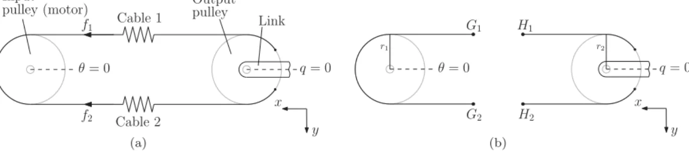
Fig. 2(a) illustrates a simple cable-based transmission composed by two antagonist cables which connect the input pulley on the motor side to the output pulley on the link side. The cables are not infinitely stiff, therefore Cable 1 is responsible for the elastic force
f1and Cable 2 is responsible for the elastic force f2. These forces are responsible for the elastic torques on the motor and link side
(namely the input and output pulleys, respectively).
In order to describe the elastic behavior in a cable-based transmission, we make the following assumption (see also[31], Chapter 4.2).
Assumption 1. Given an n-link robot manipulator actuated by p cables, the following conditions are satisfied:
•
cables have negligible mass;•
cables do not dissipate any energy (namely, there is no friction inside the cable);•
the elasticity of each cable is lumped;•
cables are not connected among them;•
cables do not slip upon surfaces.Notice that cable dynamics is in general much faster than the rest of the actuator, therefore thefirst three items ofAssumption 1
are a good approximation of a cable behavior. The fourth item is useful to keep the discussion simple and it does not exclude the most common cable-based transmissions. Finally the last item is an important requirement for the transmission to work properly. For each cable i= 1, …, , replace the lumped elasticity with two points Gp iand Hi and let g q θ( , ):n×n→p be the
displacement function of all the points Giwith i= 1, …, driven by the motor side andp h q θ( , ):n×n→pbe the displacement
function all the points Hiwith i= 1, …, driven by the link side. Indeed, displacements of Gp idepend only on the part of the
transmission linked to the motor side (ignoring the effects of the link side), whereas displacements of Hidepend only on the part of
the transmission connecting Hito the link side (ignoring the effects of the motor side). To better explain this, consider the following
example.
Example 1 (simple cable-based transmission).Fig. 2(b) illustrates how the lumped elasticity is replaced by points Giand Hiwith
i=1,2. With respect to the system of coordinates, the displacement functions associated to these points are:
(3)
The approach presented in this paper consists in modeling the effects of the elastic force of each cable at the extremities of its lumped elasticity. Points Giand Hiand their displacement functions are used to determine the elongation of the i-th cable. In
particular, the translational elongation of cables is l q θ( , )≔ ( , ) − ( , ) +g q θ h q θ lо wherelоis a constant vector, representing their
initial elongation, namely l q θ( ,о о) = ( ,g qо θо) − ( ,h qо θо) +lо=lо. The notations qо andθо refer to the motor and joint angular
positions when the cables are put in their initial elongation configuration. Thus the vector of elastic force is a function
f q θ( , ): n× n→ pwhose i-th component represents the elastic force on the i-th cable, which is given by:
⎪ ⎪ ⎧ ⎨ ⎩ f q θ f q θ δ l q θ f q θ l q θ l q θ ( , ) = ( , ) ( ( , )) = ( , ), if ( , ) > 0 0, if ( , ) ≤ 0, ∼ ∼ i i i i i i (4a) with f q θ( , ) ≔ ( , ) ( , ),k q θ l q θ ∼ i i i (4b) l q θi( , ) ≔ ( , ) −g q θi h q θi( , ) +lо,i, (4c) δ l q θ( ( , )) ≔ sgn( ( , )) + 1l q θ 2 , i i (4d) where k q θi( , )is the stiffness of the i-th cable and the constant lо,iis its initial elongation.
Cables generate elastic torque only during extension (i.e. l q θi( , ) > 0) and slack cables (unlike springs) do not produce any during compression (i.e. l q θi( , ) < 0). Indeed, (4)returns a nonzero elastic force only during positive elongation and returns 0 during compression or whenever the cable is unperturbed (i.e. l q θi( , ) = 0).
Remark 1. The elastic force in(4)depends on the cable elongation and on k q θi( , ), which represents the stiffness of the i-th cable. Notice that k q θi( , )can be a nonlinear function of the input and output positions q and θ. In order to preserve the fact that cables oppose to their elongation, we require that:
f q θ( , ) ≥ 0, ∀ ( , ) ≥ 0,l q θ i= 1, …, .p
∼
i i (5)
As a consequence, the elastic potential energy of the i-th cable is non-negative and can be expressed by:
< ⎪ ⎪ ⎧ ⎨ ⎩
∫
f q θ dl q θ∫
f q θ dl q θ l q θ l q θ = ( , ) ( , ) = ( , ) ( , ), if ( , ) > 0 0, if ( , ) ≤ 0. ∼ elas i i i i i i i (6) Remark 2. From(4) and (5), whenever q θ( , ) = ( ,qо θо)we have:f qi( ,о θо) = ( ,∼f qi о θ δ l qо) ( ( ,i о θо)) = ( ,k qi о θ lо о,) iδ l(о,i)≔fо,i ≥ 0, (7) which corresponds to the preload imposed on the i-th cable by selecting an initial elongation lо,i. Thus a strictly positive elongation
(i.e. lо,i> 0) corresponds to a taut cable whose initial elastic torque is f q θi( ,о о) > 0. Conversely a negative elongation (i.e. lо,i< 0)
means that the cable is compressed and the corresponding elastic torque is f q θi( ,о о) = 0. Finally, the case in which the cable is neither stretched nor compressed (i.e. lо,i= 0) still(7)returns zero elastic torque, namely f q θi( ,о о) = 0.
2.3. Dynamic modeling: a general elastic torque model
ConsiderAssumption 1and the definitions of g q θ( , ),h q θ( , ), l q θ( , ) with l q θ( ,о о) =lо. Then from(4) and (5), the elastic torque
on the link sideτelasl∈nand on motor sideτelasm∈ncan be expressed respectively by:
τelasl( , ) = ( , ) ( , ),q θ P q θ f q θ (8a) τelasm( , ) = ( , ) ( , ),q θ S q θ f q θ (8b) with P q θ( , )≔− g q θ h q θ ∈ q n p (∂ ( , ) − ∂ ( , )) ∂ × ⊤ andS q θ( , )≔ g q θ h q θ ∈ θ n p (∂ ( , ) − ∂ ( , )) ∂ × ⊤
being the coupling matrices that transform forces in torques and qо,θоare such that:
τelasl( ,qо θо) =τelaslо= ( ,P qо θ fо о) = 0,τelasm( ,qо θо) =τelasmо= ( ,S qо θ fо о) = 0. (8c) Eqs.(8a) and (8b)can be computed by noticing that from(1), we have:
< < ⎛ < < ⎝ ⎜ ⎞ ⎠ ⎟ ⎛ ⎝ ⎜ ⎞ ⎠ ⎟
∫
∫
∫
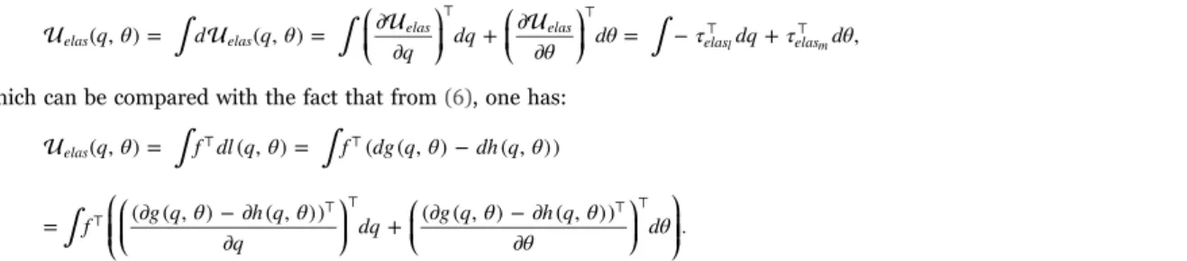
q θ d q θ q dq θ dθ τ dq τ dθ ( , ) = ( , ) = ∂ ∂ + ∂ ∂ = − + , elas elas elas elas elas elas ⊤ ⊤ ⊤ ⊤ l m (9) which can be compared with the fact that from(6), one has:<elas( , ) =q θ
∫
f dl q θ⊤ ( , ) =∫
f⊤( ( , ) −dg q θ dh q θ( , )) (10) ⎛ ⎝ ⎜⎜⎛⎝⎜ ⎞ ⎠ ⎟ ⎛ ⎝ ⎜ ⎞ ⎠ ⎟ ⎞ ⎠ ⎟⎟∫
f g q θ h q θ q dq g q θ h q θ θ dθ = (∂ ( , ) − ∂ ( , )) ∂ + (∂ ( , ) − ∂ ( , )) ∂ . ⊤ ⊤ ⊤ ⊤ ⊤ (11) Eqs.(8)allow to match elastic forces applied on the cables to the elastic torques on the link and motor side. Matrices P q θ( , ) andS q θ( , ) are functions which relate the space of elastic force coordinates to the one of elastic torque coordinates. Notice also that if
P q θ( , ) = ( , ), then τS q θ elasl=τelasm=τelas, which means that the elastic torque has the same amplitude and opposite sign in the motor
and link sides (this was the case of the linear elastic torque inSection 2.1). Condition(8c)is necessary to guarantee that the preload
f q( ,о θо) =fоon cables (or equivalently their initial elongationlо) does not generate elastic torque neither on the link nor on the
motor side. This is an important condition to guarantee the equilibrium of the dynamical system whenever only the preload is present. In other words,f ∈n
о has to be in the null space ofP q( ,о θо)and S q θ( ,о о)in such a way that P q θ f( ,о о о) = ( ,S qо θ fо о) = 0.
2.4. Functioning modes of cable-based actuators
Due to the piece-wise behavior of(4), in cable-based transmissions there might exist elastic torques τelasl, τelasmand( , )q θ pairs
such that fi=0 for some i= 0, …, . In particular, we distinguish two separate cases:p
a. force-closure case: givenτelasl,τelasm∈n, for eachq θ, ∈
nthere exists a set of forces f∈psuch that(8)holds and
f q θi( , ) > 0, ∀ = 0, …, ;i p (12)
b. force-disclosure case: givenτelasl,τelasm∈n, for eachq θ, ∈
nthere exists a set of forces f∈psuch that(8)holds and
f q θi( , ) ≥ 0, ∀ = 0, …, ,i p (13)
and there exists at least one j= 0, …, such that f q θp j( , ) = 0.
The force-closure case has been widely used in previous works, see for instance [31,34] and implies that all the cables are simultaneously taut (see, for instance,Fig. 3(b)). Here we are completing cable-based transmissions behavior by introducing the force-disclosure case, where at least one of the cables is relaxed (seeFig. 3(c)). These two cases depend on: the required elastic torques, the positionq θ, and the preload tuned in the cables in the assembly phase.
In general, there is no a priori preference between the two cases a and b or even between force-closure and force-disclosure networks. Typically, force closure cases have the advantage to reject low frequencies vibrations, although undesired friction effects amongst cables and rigid solid bodies such as pulleys are usually more significant. On the other hand, force disclosure cases restraint such friction effects but might present low frequencies vibrations. Force-closure networks are typical in robotic hand applications where the cables are called elastic tendons (see[31], Chapter 4.1 for more details). However, other robotic applications may prefer the force-disclosure functioning mode or may even exhibit both functioning modes (seeSection 4). This is why we complete the definition of force closure by adding case b.
Here next, we present an example to show how to use the framework we introduced so far.
Example 2 (design of a 2-cable network). RecallExample 1andFig. 2.Fig. 3shows the example of a cable-based transmission composed by an input pulley and an output pulley, interconnected by two antagonist cables (hence p=2) supposed equal and not infinitely stiff. The input pulley is supposed rigidly connected to the motor side (eventually with some reduction gear stages), whereas the output pulley is connected to the robot link (and eventually to a load). The gravity force is oriented along with the z axes so that gravity is not effective. According to[28](see alsoSection 2.1), the dynamics of a 1-DOFflexible robot is represented by:
J qM¨ +τfl( ̇) =q τelasl( , ) +q θ τload (14a)
J θm¨ +τfm( ̇) +θ τelasm( , ) =q θ τ (14b)
withJM∈the rigid body inertia,Jm∈the actuator inertia,τfl( ̇),q τfm( ̇) ∈θ the link and motor friction torques,τelasl( , ) ∈q θ
Fig. 3. Functioning modes in a cable-based transmission. (a) Preload in force-closure case. (b) Still force-closure case. (c) Force-disclosure case. (d) Symmetry of functioning modes.
andτelasm( , ) ∈q θ the link and motor elastic torques,τload∈the load torque andτ∈the motor control torque. For sake of
clarity and without loss of generality, let us assume that the pulleys have the same radius r. From (3) we have that
P q θ( , ) = ( , ) = [ , − ], which implies τS q θ r r elas=τelasl=τelasmto(14). Moreover from(8), we have:
τelas= ( − ),r f1 f2 (15)
where f1and f2are defined in(4), with l q θ1( , ) = ( − ) +r θ q lо,1, l q θ2( , ) = − ( − ) +r θ q lо,2and their stiffness k q θ1( , ) =k q θ2( , )will
be selected later.Consider nowFig. 3(a) with q θ( , ) = ( ,qA θA)such that g q( ,A θA) = ( ,h qA θA) = 0(namely, there is no displacement due
to the pulleys) and control torque τA= 0. If the system is at the equilibrium with respect to(14)(namely, q̇ = ¨ = ̇ = ¨ = 0), itq θ θ follows that τA=τelas= −τloadA= 0. Moreover, we have l qi( ,A θA) =lо,iand from(7), we get f qi( ,A θA) = ( ,k qi A θ lA)о,iδ l(о,i) =fо,i ≥ 0,
with i=1,2. Notice also that(8c)implies f q1( ,A θA) =fо,1=fо,2= ( ,f q2 A θA), hence lо,1=lо,2. This study shows that at the equilibrium
the preload fо does not affect the elastic torque τelas. Moreover if fо,1=fо,2> 0, the transmission satisfies the force-closure
condition(12), otherwise if fо,1=fо,2= 0the transmission satisfies the force-disclosure condition(13).ConsiderFig. 3(b) where a constant control torque τB> 0is applied and the new equilibrium point q θ( ,B B)is such that τB=τelas= −τloadB> 0. From(15), we
have τelas= ( ( ,r f q1 B θB) − ( ,f q2 B θB)) > 0, thus f q θ1( ,B B) − ( ,f q2 B θB) > 0, which implies l q θ1( ,B B) > ( ,l q1 A θA)and l q2( ,A θA) < ( ,l q2 B θB).
In other words, Cable 1 is more stretched with respect toFig. 3(a) so that f q θ1( ,B B) ≥ ( ,f q1 A θA) > 0and conversely, Cable 2 is less stretched so that f q θ2( ,B B) ≤ ( ,f q2 A θA). In this case, if f q θ2( ,B B) > 0then the force-closure condition(12)is still satisfied although the
elastic torque contribution of the cables is unbalanced, otherwise Cable 2 is completely relaxed and does not provide any contribution to the elastic torque according to the force-disclosure condition(13).Fig. 3(c) shows the case where a constant control torque τC>τBis provided, so that Cable 2 is completely relaxed (namely f q2( ,C θC) = 0) and the force-disclosure condition(13)is
satisfied. In particular,(15)returns τelas=τloadc=rf1, moreover since f2 = 0we have l q2( ,C θC) ≤ 0, that is θC−qC≥lо,2/r(notice that
the inverse situation where only Cable 2 contributes to τelas is also possible).Finally Fig. 3(d) resumes that force closure is
guaranteed up to a certain threshold of input torque τBand higher magnitudes of torque leads to force disclosure.
3. Polynomial stiffness and identification
3.1. Polynomial elastic torque model
By applying the framework presented in Section 2, we propose a polynomial elastic stiffness for each cable. Based on experimental results, we infer a piece-wise polynomial elastic torque model which can be embedded in the dynamical model and is suitable for identification through classical methods. The order of the considered polynomial approximation in the approximant is controlled. This provides a good match with numerical computation, since it represents closely the cost of computation (number of operations). The number of parameters usually correlates well with computational effort.
RecallAssumption 1and(4), then in(4b)the polynomial function l q θi( , )↦ ( , )k q θi of the i-th cable stiffness can be expressed by:
∑
k q θi( , )≔ k l q θ( , ) ≥ 0, ∀ ( , ) ≥ 0,l q θ j d i j i j i =0 , i (16) where di∈ Nis the polynomial degree andki j, are real polynomial coefficients. Thus,(4)can be particularized in the followingcompact form:
∑
∑
f q θi( , ) = ( , ) ( , ) ( ( , )) =k q θ l q θ δ l q θi i i k l q θ( , ) δ l q θ( ( , )) = k σ l q θ( ( , )) j d i j i j i j d i j i j =0 , +1 =0 , +1 i i (17) with σ l q θ( ( , ))≔ ( , ) ( ( , )),i l q θ δ l q θi i (18)where we used the fact that δ l q θ( ( , )) = ( ( , ))i δ l q θi i for any i∈ N and l q θi( , ) ≠ 0(recall that l q θi( , ) = 0alone implies σ q θ( , ) = 0
and hence f q θi( , ) = 0).
Notice that the fact that(16)is positive definite for all l q θi( , ) ≥ 0guarantees(5)and hence, the passive nature of the elasticity of each cable(6)(seeRemark 1).
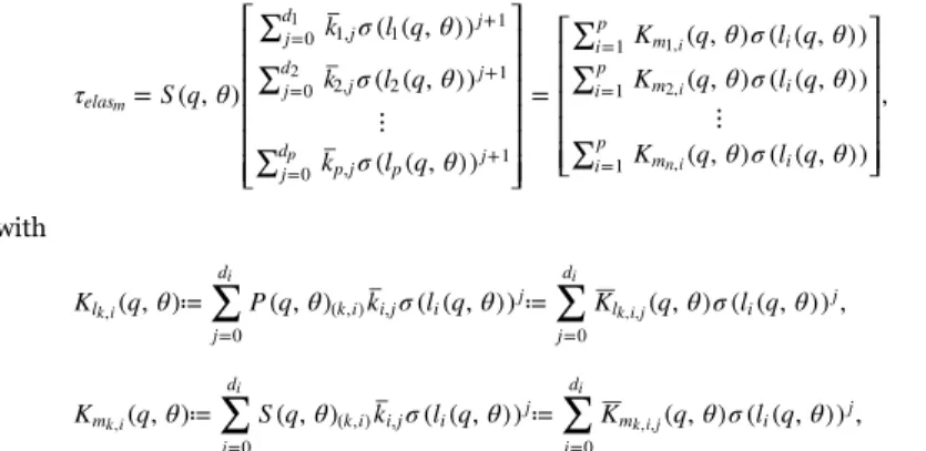
From(4), (8) and (16), the corresponding piece-wise polynomial elastic torques τelasland τelasmare expressed respectively by:
⎡ ⎣ ⎢ ⎢ ⎢ ⎢ ⎢ ⎢ ⎤ ⎦ ⎥ ⎥ ⎥ ⎥ ⎥ ⎥ ⎡ ⎣ ⎢ ⎢ ⎢ ⎢ ⎢ ⎤ ⎦ ⎥ ⎥ ⎥ ⎥ ⎥ τ P q θ k σ l q θ k σ l q θ k σ l q θ K q θ σ l q θ K q θ σ l q θ K q θ σ l q θ = ( , ) ∑ ( ( , )) ∑ ( ( , )) ⋮ ∑ ( ( , )) = ∑ ( , ) ( ( , )) ∑ ( , ) ( ( , )) ⋮ ∑ ( , ) ( ( , )) , elas j d j j j d j j j d p j p j i p l i i p l i i p l i =0 1, 1 +1 =0 2, 2 +1 =0 , +1 =1 =1 =1 l p i i n i 1 2 1, 2, , (19a)
⎡ ⎣ ⎢ ⎢ ⎢ ⎢ ⎢ ⎢ ⎤ ⎦ ⎥ ⎥ ⎥ ⎥ ⎥ ⎥ ⎡ ⎣ ⎢ ⎢ ⎢ ⎢ ⎢ ⎤ ⎦ ⎥ ⎥ ⎥ ⎥ ⎥ τ S q θ k σ l q θ k σ l q θ k σ l q θ K q θ σ l q θ K q θ σ l q θ K q θ σ l q θ = ( , ) ∑ ( ( , )) ∑ ( ( , )) ⋮ ∑ ( ( , )) = ∑ ( , ) ( ( , )) ∑ ( , ) ( ( , )) ⋮ ∑ ( , ) ( ( , )) , elas j d j j j d j j j d p j p j i p m i i p m i i p m i =0 1, 1 +1 =0 2, 2 +1 =0 , +1 =1 =1 =1 m p i i n i 1 2 1, 2, , (19b) with
∑
∑
Kl ( , )≔q θ P q θ( , ) k σ l q θ( ( , )) ≔ K ( , ) ( ( , )) ,q θ σ l q θ j d k i i j i j j d l i j =0 ( , ) , =0 k i i i k i j , , , (19c)∑
∑
Km ( , )≔q θ S q θ( , ) k σ l q θ( ( , )) ≔ K ( , ) ( ( , )) ,q θ σ l q θ j d k i i j i j j d m i j =0 ( , ) , =0 k i i i k i j , , , (19d) where di> 0is the degree of the polynomial elastic stiffness of the i-th cable and the initial elongation lо,i, satisfies condition(8c),that is:
∑ ∑
ip dj Kl ( ,q θ σ l) ( i)j = 0,∑ ∑
K ( ,q θ σ l) ( ) = 0. i p j d m i j =1 =0 о о о, +1 =1 =0 о о о, +1 i k i j i k i j , , , , (19e)Eqs.(19c) and (19d)represent the polynomial stiffness due to the i-th cable on the link side and motor side, respectively. Notice that such stiffness is torsional for rotational joints and axial for translational ones. Indeed, Klk i,( , )q θ, Kmk i,( , )q θ andKlk i j, ,( , )q θ,
Kmk i j, ,( , )q θ are polynomial functions of the elongation l q θi( , )and diis the polynomial degree of the polynomial stiffness k q θi( , )
associated to the i-th cable.
As compared toSection 2.1, the case of linear elasticity (see(2b) and (2c)) is a particular case of(19)and it can be retrieved by selecting p=2, di=0, Klk,1=Kmk,1=Kk, Klk,2=Kmk,2= −Kk, l q θ1( , ) = − ( , ) = −l q θ2 θ qand lо,1=lо,2= 0for all k= 1, …, .n
Example 3 (comparison of linear and polynomial stiffness). ConsiderExamples 1 and 2andFigs. 1–3. If each cable has linear stiffness, then(4) and (16)(with d1=d2= 1) yields:
f1,lin=k1,0 1l q θ δ l q θ( , ) ( ( , )),1 (20a)
f2,lin=k2,0 2l q θ δ l q θ( , ) ( ( , )).2 (20b) On the other hand, if in case of a second order polynomial stiffness(4) and (16)(with d1=d2= 2) yields:
f1,pol= (k1,0 1l q θ( , ) +k l q θ1,1 1( , ) ) ( ( , )),2 δ l q θ1 (21a)
f2,pol= (k2,0 2l q θ( , )) +k l q θ2,1 2( , ) ) ( ( , ))).2 δ l q θ2 (21b) Thus by applying (15), we are able to compare the piece-wise elastic torque with the classical linear elastic torque (2). Fig. 4
Fig. 4. Comparison of the linear elastic torque (solid line), linear and piece-wise elastic torque (dashed line), polynomial and piece-wise elastic torque (dashed-dot bold line). p=2 and lо,1=lо,2.
qualitatively compares the trend of several types of elastic torque model (for sake of clarity, we are assumingτelasl=τelasm=τelas∈).
The classical linear elastic torque (seeSection 2.1) represented by the solid line, does not take into account any preload. Instead by using(19), we can assume linear elastic force on each cable (namely di=0 for all i= 1, …, , kp = 1, …, ) and take into account an
preload, which implies a piece-wise trend of the elastic torque represented by the dashed line. Indeed the gray zone inFig. 4
represents the area where the force-closure case is satisfied whereas the white zones represent the area where the force-disclosure case is satisfied instead. Finally, the dashed-dot bold line shows the case where polynomial stiffness on each cable is considered in
(19) (see Section 4for more details). Notice that for the piece-wise models, the contribution of each cable is independently considered, thus the white areas on the sides represent the force-disclosure zones when only one cable at the time is taut. Moreover, the classical linear elastic model does not consider preload and cannot really approximate the trends of the two piece-wise elastic models. We anticipate now that in the experimental result section, we will show that the polynomial stiffness suits better the stiffness in certain conditions.
3.2. Identification
Robot identification is an important step for the design of hybrid force/position control strategies[35], Chapter 7 and collision detection algorithms[36]. Here next, we briefly present the parameter identification of flexible robot models. The reader is referred to[16]for more exhaustive guidelines.
Be the robot rigid or flexible, the main idea for the identification relies on the linear dependency between the unknown parameters and state and measurements of the model[37–41]. Therefore the dynamical model of aflexible robot can be equivalently written as[28]:
Y=W q q q θ θ θ Λ( , ̇, ¨, , ̇, ¨) , (22)
where Y is the measurement vector (τloadis usually known during identification tasks), W q q q θ θ θ( , ̇, ¨, , ̇, ¨) is the regression matrix, Λ
is the vector of the unknown parameters. Now let lΛ be the estimate of Λ, then we can define the identification error l
ρ=Y−W q q q θ θ θ Λ( , ̇, ¨, , ̇, ¨) . Typically, the purpose of identification algorithms is to calculate lΛ on the basis of measurements of ρ, Y and W. Indeed, an effective algorithm is the least-squares algorithm (LSA), which minimizes the 2-norm of the identification error ρ.
Ordinary least-squares technique is used to estimate parameters solving an over-determined linear with respect to parameters system obtained from a sampling of the dynamic model, along a given trajectory W q q q θ θ θ( , ̇, ¨, , ̇, ¨). In practice, W is a a× full rankb
and well-conditioned matrix, obtained by tracking exciting trajectories and by considering parameters, a being the number of samplings along a given trajectory,a b⪡ . Hence, the estimate of Λ that minimizes the 2-norm identification error is:
l
Λ = ((W WT )−1WT) =Y W Y+ (23)
with W+the pseudo-inverse matrix of W. Then, the standard deviations of the identified parameters,σl
Λj, are estimated using classical
and simple results from statistics considering that the matrix W is deterministic and that the error vector ρ is assumed to be a zero-mean additive independent noise, with standard deviation σρsuch that:
Cρρ= E[ρ ρT ] =σ Iρ2 (24)
whereE[·] is the expectation operator, and I the identity matrix. The variance-covariance matrix of the standard deviation is calculated as follows:
l l
CΛ Λ=σρ2(W WT )−1 (25)
Then,σΛl2j=Cl lΛ Λj jjis the j-th diagonal coefficient ofCl lΛ Λ.
For more details on the LS algorithm, the reader is referred to[42] for the direct formulation (D-LSA) and to[43] for the recursive formulation (R-LSA). Further algorithms can be found in the references therein. The piece-wise polynomial elastic torque presented in(19)has yet the advantage to preserve the linear relationship between the parameterski j, and the robot state position
q θ
( , )(through the l q θi( , )). Thus the classical identification strategy briefly introduced above still holds and in particular(22)can be expressed by: Y≔ [τload⊤ 0 0 τ⊤ ⊤] , (26) ⎡ ⎣ ⎢ ⎢ ⎢ ⎢ ⎢ ⎤ ⎦ ⎥ ⎥ ⎥ ⎥ ⎥ W q θ W q q q W q θ W q θ W q θ W q θ W θ θ θ ( , …, ¨) ≔ ( , ̇, ¨) ( , ) 0 0 0 ( , ) 0 0 0 0 ( , ) 0 0 0 ( , ) ( , ̇, ¨) , l elas elas elas elas m о о о о l l m m (27) Λ≔ [Λl⊤ Λelas⊤l Λelas⊤ m Λm⊤⊤], (28)
where Wl and Wm are the link and motor regressors, respectively, which are unrelated with the elastic torque model,
τelasl=Welasl( , )q θ Λelasl, τelasm=Welasm( , )q θ Λelasm where each component of τelasl, τelasm comes from (19), and
We emphasize that the identification concerns the estimation of the parameterski j, in(19c)–(19d)and that an initial guess (or a
line-search) needs to be performed on the initial elongation of each cable lо,i, if unknown. Indeed, lо,iis injected in the sgn function in
(19)(see also(4)) and therefore it cannot be estimated through linear techniques. However, an empirical guess or a line-search upon
lо,idoes not affect the usefulness of our model and the enhancement of precision with respect to classical techniques. Moreover, in
the next section we will present a twist in the parameter estimation which involves a two-step identification which allows to avoid an a priori guess upon lо,i.
4. Identification and experimental results
In previous examples we showed that the framework allows to generate a model in order to predict the behavior of the cable-based transmission and helping the choice of the designer to satisfy all the specifications. In this section, we want to illustrate:
•
the advantages in the numerical model. We present the identification of a cable-based transmission and we show that piece-wise polynomial behavior is better than linear one and that the approximation error due to a linear elastic model can be quantified;•
the effects of the preload. We show how, given a constant load, varying the preload will affect the cable elongation, the frictionsbetween the taut cables and the pulleys integrated in the chain robot, and the efficiency of the whole transmission.
4.1. Identification phase: a ball-screw cable-based actuator
Fig. 5shows a cable-based transmission developed at CEA Interactive Robotics Laboratory[44], whose sketch could be found in
Figs. 2 and 3. The assembly is realized by using the cables to link the output pulley to a nut which is engaged on a ball screw and its mechanical principle is briefly described as follows. The electric motor transmits a rotational movement to the ball screw. Since the latter is only free to rotate, the nut engaged on it will be only able to translate along its axes, transmitting the movement to the cables and thus to the output pulley. Notice that the complete transmission needs two antagonist ball screws ball-screws in order to supply output torque on both ways. The motor position θ is associated to the ball screw to include the gear ratio and the link position q corresponds to the output pulley position to which the link is rigidly connected. The motor-ball screw coupling is considered stiff. Instead, each considered cable is a multi-strand (flexible) cable, that is attached to the ball-screw, can be stretched and relaxed and are the source offlexibility of the actuator. A motor from has been chosen to power the actuation system due to their simplicity of operation. Both position and current measurements are allowed with its associated drive device for motor control. It is equipped with a standard AKM resolver for position feedback to record the angular position at the motor (transmission input) level. The joint angle measurement is made using a position encoders directly mounted on the joint shaft for absolute (transmission output) measurement of the joint.
Now we are ready to make the identification of the parameters in(14)associated to the cable-based transmission presented above. As anticipated at the end ofSection 3, we present a two-step identification. First, we estimate the elastic model by applying position references to the motor with the output pulley blocked (namely, q=0) and measuring the control torque τ. Then, we identify the remaining parameters with the classical least-square identification algorithms. This two-step identification presents the advantage of isolating the parameters of the elastic model and does not need a guess upon li,о.
4.1.1. Elastic model estimation
Recall that q is blocked in q=0 and moreover, θ is controlled by a classical position PD controller which generates the control torque τ.Figs. 6 and 7present values of τ as a function of θ at the equilibrium (hence τ=τelasaccording to(14)), in case of two
different preloads, respectively.
For each preload, we make an optimal second order polynomial approximation and an optimal linear approximation in a least-square sense, in order to link τelasvalues to θ−qdeflections. For the linear case, the elastic torque model is: (seeSection 2.1):
τelas=K θ( − ),q (29)
withK∈the linear stiffness to be identified. For the second degree polynomial case,(15) and (21)with l1,о=l2,о= 0yield:
τ r f f r k r θ q k r θ q δ θ q k r q θ k r q θ δ q θ k r θ q k r θ q δ θ q k r q θ k r q θ δ q θ K θ q K θ q δ θ q K q θ K q θ δ q θ = ( − ) = [( ( − ) + ( − ) ) ( − ) − ( ( − ) + ( − ) ) ( − )] = ( ( − ) + ( − ) ) ( − ) − ( ( − ) + ( − ) ) ( − ) = ( ( − ) + ( − ) ) ( − ) − ( ( − ) + ( − ) ) ( − ),
elas 1,pol 2,pol 1,0 1,1 2 2 2,0 2,1 2 2
1,0 2 1,1 3 2 2,0 2 2,1 3 2
1,0 1,1 2 2,0 2,1 2 (30)
withK1,0,K1,1∈the coefficients of the second order polynomial stiffness of cable 1 and K2,0,K2,2∈the coefficients of the second
order polynomial stiffness of cable 2, all to be identified.
Indeed, for the polynomial stiffness in (16), if l1,о=l2,о= 0 then from(21) we have f1,poly > 0 wheneverθ−q> 0, whereas
f2,poly > 0wheneverθ−q< 0. Thus to estimate the polynomial elastic torque model, we impose l1,о=l2,о= 0and according to(15),
we let f1,poly and−f2,poly approximate only the positive and negative values of τelas=τ, respectively. This has the advantage of not
requiring a guess upon l1,оand l2,оwithout renouncing to the quality of the results.
Table 1presents the identified elastic parameters for the linear and polynomial model in both cases with low and high preload. In the case of low preload (seeFig. 6), one can see that τelashas a nonlinear trend which is well represented by the polynomial
stiffness. Indeed,Fig. 6(b) shows that the polynomial model introduces an error of max10 , whereas the linear model can go up toN
Table 1
Stiffness identification summary.
Linear Polynomial (d1=d2= 2) Preload K [N m rad−1] K1,0[N m rad−1] K 1,1[N m rad−2] K 2,0[N m rad−1] K 2,1[N m rad−2] Low: K=1819.2 1367.7 37,844.1 1575.3 29,357.2 High: K=3605.2 −3894.7 3891.4 11,171.0 3094.9
Fig. 6. Low preload case: comparison between polynomial elastic model and linear model (q=0). (a) Measured elastic torque (τelas), estimated polynomial piece-wise
N
70 in the deflection range of interest. In the case of high preload (seeFig. 7), τelas has a quite linear trend which is well
approximated both by the polynomial and by the linear model.Fig. 7(b) shows that there is not relevant difference in the estimated elastic torque error. This concludes thefirst step of the identification.
4.1.2. Model identification
In this section, we estimate the remaining parameters (JM, Jm, τfaand τfm) in(14)also considering the classical Coulombs-like
friction effects represented by:
τfa=f qv ̇ + sgn( ̇) andfs q τfm=fvmθ̇ +fsmsgn( ̇).θ (31)
Note that the friction effects that the authors are referring to here is the friction amongst rigid solid bodies that constitute the chain robot manipulator. It is not refering to friction inside the cable, as it is stated inAssumption 1(second item) that cables are not dissipating any energy in our study.Fig. 5shows a mass of about 40 kg which is connected to the link through an inelastic rope and a system of external pulleys. Indeed, the load torque is known and is a function of the link position, namely q τ↦load( )q. We use the
elastic models estimated in the previous section and we use the least-mean square algorithm to estimate the remaining parameters.
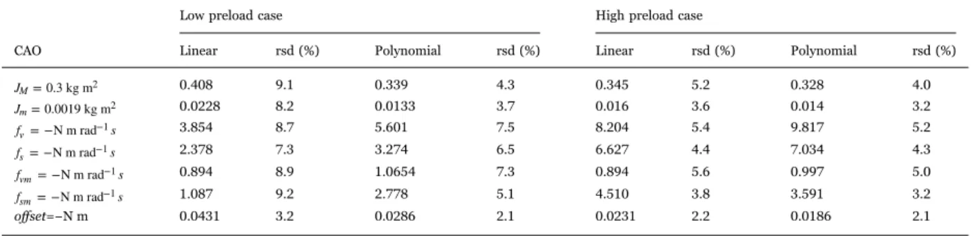
Table 2resumes the identified values for the polynomial and linear case with their relative standard deviation in presence of low preload and high preload settings, respectively. Notice that in case of low preload, the error of the linear model is not negligible and the variance of some parameters from the CAO values is important. On the contrary, the polynomial elastic model is enough precise and the identified parameters are closer to the CAO values. In case of high preload, the variance of the estimated parameters is comparable between the polynomial and the linear case.Figs. 8 and 9propose the torque estimation error with low preload and high preload respectively. As expected, the error introduced by the linear model in case of low preload does not make it suitable to some applications (i.e.collision detection), whereas the polynomial model seems more precise. On the opposite,Fig. 9shows that with high preload, both polynomial and linear elastic models are suitable for collision detection algorithms.
Fig. 7. High preload case: comparison between polynomial elastic model and linear model (q=0). (a) Measured elastic torque (τelas), estimated polynomial
Table 2
Dynamic identification summary (estimated values with their relative standard deviation – rsd – in (%)).
Low preload case High preload case
CAO Linear rsd (%) Polynomial rsd (%) Linear rsd (%) Polynomial rsd (%)
JM= 0.3 kg m2 0.408 9.1 0.339 4.3 0.345 5.2 0.328 4.0 Jm= 0.0019 kg m2 0.0228 8.2 0.0133 3.7 0.016 3.6 0.014 3.2 fv= −N m rad−1s 3.854 8.7 5.601 7.5 8.204 5.4 9.817 5.2 fs= −N m rad−1s 2.378 7.3 3.274 6.5 6.627 4.4 7.034 4.3 fvm= −N m rad−1s 0.894 8.9 1.0654 7.3 0.894 5.6 0.997 5.0 fsm= −N m rad−1s 1.087 9.2 2.778 5.1 4.510 3.8 3.591 3.2 offset=−N m 0.0431 3.2 0.0286 2.1 0.0231 2.2 0.0186 2.1
Fig. 8. Low preload.
5. Conclusions
In this paper, a framework to model elastic behavior of cable-based transmissions has been presented. We used analytical mechanics to infer the elastic model and we introduced the concept of force-disclosure case. Moreover, we dealt with the identification problem and we showed that in case of polynomial elastic stiffness the classical least-square based methods are still suitable. Theoretical results are generalized to multi-axes robots, since all the mathematical developments are related to the multivariable case. Finally, the concept of preload has been introduced and experimental investigations, that were conducted on 1-dofflexible robot, illustrated that the case of cables with low preload values are not faithfully represented by linear elastic models as it is commonly used. On the opposite, classical linear stiffness models become more reliable in the case of high preload values. The tradeoff between these extreme cases is a crucial aspect in machine control and design: the authors hope that this work may help the development of simple but yet more precise numerical models and control techniques. Indeed, control issues inherited from the rigid robotics are worsened due to the risingflexibility. Although several control strategies initially proposed for the control of rigid robot have been extended toflexible robots [45–47], the problem of tracking control, robustness, vibration damping and collision detection require accurate dynamical models in order to characterize and predict the robot behavior.
Future works aim tofind better elastic models than the polynomial one investigated in this paper. Others techniques could be tried, such as wavelets or even optimal basis selection and greedy algorithms (adaptive pursuit). Moreover, the extension of this approach to the case of interconnected cables is also of interest for several applications. Yet, new identification algorithms might suit better the parameter estimation of more sophisticated models.
Appendix
In case of polynomial stiffness of degree difor each i-th cable, with i= 1, …, , we have:p
τelasl=Welasl( , )q θ Λelasl= ( , )P q θ Φelas( , )q θ Λelas, (32a)
τelasm=Welasm( , )q θ Λelasm= ( , )S q θ Φelas( , )q θ Λelas, (32b)
(32c)
Λelas≔[K1,0 K1,1… K1,r1 K2,0 K2,1 … K2,r2 … Kp,0 Kp,1 … Kp r,p] ,⊤ (32d) notice that in (32c) we omitted the dependencies on q and θ for reason of space. Notice that typically matrices P q θ( , ) and S q θ( , ) are known from the direct geometrical model of the robot and eventual unknown parameters therein can be embedded in the parameter vector yielding Λelasland Λelasm.
References
[1] M. Makarov, M. Grossard, P. Rodriguez-Ayerbe, D. Dumur, Modeling and preview hinf control design for motion control of elastic joint robots with uncertainties, IEEE Trans. Ind. Electron. PP (99) (2016) 1.http://dx.doi.org/10.1109/TIE.2016.2583406.
[2] S. Wolf, A. Albu-Schäffer, Towards a robust variable stiffness actuator, in: Proceedings of 2013 IEEE/RSJ International Conference on Intelligent Robots and Systems, 2013, pp. 5410–5417.
[3]E. Nazma, S. Mohd, Tendon driven robotic hands: a review, Int. J. Mech. Eng. Robot. Res. 1 (2012) 1520–1532.
[4]D.-g. Zhang, Recursive lagrangian dynamic modeling and simulation of multi-link spatialflexible manipulator arms, Appl. Math. Mech. 30 (10) (2009) 1283–1294.
[5]C. Damaren, I. Sharf, Simulation offlexible-link manipulators with inertial and geometric nonlinearities, J. Dyn. Syst. Meas. Control 117 (1) (1995) 74–87. [6] L. Zollo, B. Siciliano, C. Laschi, G. Teti, P. Dario, Compliant control for a cable-actuated anthropomorphic robot arm: an experimental validation of different
solutions, in: Proceedings of IEEE International Conference on Robotics and Automation, 2002. ICRA '02, vol. 2, 2002, pp. 1836–1841.
[7]G. Piras, W. Cleghorn, J. Mills, Dynamicfinite-element analysis of a planar high-speed, high-precision parallel manipulator with flexible links, Mech. Mach. Theory 40 (7) (2005) 849–862.
[8]G. Alici, B. Shirinzadeh, Enhanced stiffness modeling, identification and characterization for robot manipulators, IEEE Trans. Robot. 21 (4) (2005) 554–564. [9] G. Carbone, Stiffness performance of multibody robotic systems, in: Proceedings of 2006 IEEE International Conference on Automation, Quality and Testing,
Robotics, vol. 2, 2006, pp. 219–224.
[10] G. Carbone, Stiffness analysis and experimental validation of robotic systems, Front. Mech. Eng. 6 (2) (2011) 182–196.
[11] M.H. Ang, G.B. Andeen, Specifying and achieving passive compliance based on manipulator structure, IEEE Trans. Robot. Autom. 11 (4) (1995) 504–515. [12] Y. Li, S.-F. Chen, I. Kao, Stiffness control and transformation for robotic systems with coordinate and non-coordinate bases, in: Proceedings of IEEE
International Conference on Robotics and Automation, 2002. ICRA '02, vol. 1, 2002, pp. 550–555.
[14] S. yoon Jung, S. kyun Kang, M.-J. Lee, I. Moon, Design of robotic hand with tendon-driven threefingers, in: Proceedings of International Conference on Control, Automation and Systems. ICCAS '07, 2007, pp. 83–86.
[15]J. Martin, M. Grossard, Design of a fully modular and backdrivable dexterous hand, Int. J. Robot. Res. 33 (5) (2014) 783–798.
[16]M. Makarov, M. Grossard, Modeling and motion control of serial robots, in: M. Grossard, N. Chaillet, S. Régnier (Eds.), Flexible Robotics: Applications to Multiscale Manipulations, Wiley, 2013, pp. 275–319.
[17]L. Zollo, S. Roccella, E. Guglielmelli, M. Carrozza, P. Dario, Biomechatronic design and control of an anthropomorphic artificial hand for prosthetic and robotic applications, IEEE/ASME Trans. Mechatron. 12 (4) (2007) 418–429.
[18]M. Luo, G. Carbone, M. Ceccarelli, X. Zhao, Analysis and design for changingfinger posture in a robotic hand, Mech. Mach. Theory 45 (6) (2010) 828–843. [19]J. Martin, M. Grossard, Mechanicalflexibility and the design of versatile and dexterous grippers, in: M. Grossard, N. Chaillet, S. Régnier (Eds.), Flexible
Robotics: Applications to Multiscale Manipulations, Wiley, 2013, pp. 145–180.
[20] Y. Yang, W. Chen, X. Wu, Q.Chen, Stiffness analysis of 3-dof spherical joint based on cable-driven humanoid arm, in: Proceedings of the 5th IEEE Conference on Industrial Electronics and Applications (ICIEA), 2010, pp. 99–103.
[21] X. You, Z. Xu, W. Chen, S. Yu, Y. Jin, Dynamic modeling and tension analysis of a 7-dof cable-driven robotic arm, in: Conference Anthology, IEEE, 2013, pp. 1– 6.
[22] M. Makarov, M. Grossard, P. Rodriguez-Ayerbe, D. Dumur, Active damping strategy for robust control of aflexible-joint lightweight robot, in: Proceedings of 2012 IEEE International Conference on Control Applications (CCA), 2012, pp. 1020–1025.
[23]J. Zhao, B. Xie, C. Song, Generating human-like movements for robotic arms, Mech. Mach. Theory 81 (2014) 107–128. [24]G. Costello, Theory of Wire Rope, Mechanical Engineering Series, Springer, New York, 1997.
[25]W. Lacarbonara, A. Pacitti, Nonlinear modeling of cables withflexural stiffness, J. Math. Probl. Eng. 21 (Article ID 370767) (2008) 1–17. [26] A. Love, A Treatise on the Mathematical Theory of Elasticity, Cambridge University Press, Cambridge, 2013 URL: 〈https://books.google.fr/books?
id=JFTbrz0Fs5UC〉.
[27] W. Seemann, Deformation of an elastic helix in contact with a rigid cylinder, Arch. Appl. Mech. 67 (1) (1996) 117–139.http://dx.doi.org/10.1007/ BF00787145.
[28]A..D. Luca, W. Book, Robots withflexible elements, in: B. Siciliano, O. Khatib (Eds.), Springer Handbook of Robotics, Springer, 2008, pp. 287–319. [29]R. Kelly, D. Santibáñez, P. Loría, Control of Robot Manipulators in Joint Space, Springer, London, 2006.
[30]P. Tomei, A simple PD controller for robots with elastic joints, IEEE Trans. Autom. Control 36 (10) (1991) 1208–1213. [31]R. Murray, Z. Li, S. Sastry, A Mathematical Introduction to Robotic Manipulation, CRC Press, Boca Raton, 1994.
[32]A..D. Luca, B. Siciliano, L. Zollo, PD control with on-line gravity compensation for robots with elastic joints: theory and experiments: theory and experiments, Automatica 41 (10) (2005) 1809–1819.
[33]M. Spong, S. Hutchinson, M. Vidyasagar, Robot Modeling and Control vol. 3, Wiley, New York, 2006.
[34]X. Diao, O. Ma, A method of verifying force-closure condition for general cable manipulators with seven cables, Mech. Mach. Theory 42 (12) (2007) 1563–1576. [35]B. Siciliano, O. Khatib, Springer Handbook of Robotics, Springer, Berlin, 2008.
[36]B. Huard, M. Grossard, S. Moreau, T. Poinot, Position estimation and object collision detection of a tendon-driven actuator based on a polytopic observer synthesis, Control Eng. Pract. 21 (9) (2013) 1178–1187.
[37]W. Khalil, E. Dombre, Modeling, Identification and Control of Robots, Butterworth-Heinemann, Oxford, 2004.
[38] M. Pham, M. Gautier, P. Poignet, Identification of joint stiffness with bandpass filtering, in: Proceedings of IEEE International Conference on Robotics and Automation. 2001 ICRA, vol. 3, IEEE, 2001, pp. 2867–2872.
[39]E. Wernholt, S. Gunnarsson, Nonlinear Grey-box Identification of Industrial Robots Containing Flexibilities, Linköping University Electronic Press, Sweden, 2004.
[40] M. Makarov, M. Grossard, P. Rodriguez-Ayerbe, D. Dumur, A frequency-domain approach forflexible-joint robot modeling and identification, in: Proceedings of SYSID2012, vol. 16, 2012, pp. 583–588.
[41]A. Klimchik, B. Furet, S. Caro, A. Pashkevich, Identification of the manipulator stiffness model parameters in industrial environment, Mech. Mach. Theory 90 (2015) 1–22.
[42]G. Golub, C..V. Loan, Matrix Computations vol. 3, Johns Hopkins University Press, Baltimore, MD, USA, 2012.
[43]S. Sastry, M. Bodson, Adaptive Control: Stability, Convergence and Robustness, Courier Corporation, Upper Saddle River, NJ, USA, 2011. [44] P. Garrec, F. KFOURY, Misalignment-tolerant cable actuator, wO Patent App. PCT/EP2014/053,258, Aug. 28 2014.
[45]M. Spong, Modeling and control of elastic joint robots, J. Dyn. Syst. Meas. Control 109 (4) (1987) 310–318.
[46] S. Nicosia, P.Tomei, On the feedback linearization of robots with elastic joints, in: Proceedings of the 27th IEEE Conference on Decision and Control, 1988, pp. 180–185.
![Fig. 5 shows a cable-based transmission developed at CEA Interactive Robotics Laboratory [44], whose sketch could be found in Figs](https://thumb-eu.123doks.com/thumbv2/123doknet/13162743.390021/11.816.250.571.82.251/shows-cable-transmission-developed-interactive-robotics-laboratory-sketch.webp)