A Characterization of Lyapunov Inequalities
for Stability of Switched Systems
The MIT Faculty has made this article openly available.
Please share
how this access benefits you. Your story matters.
Citation
Junger, Raphael M., Amirali Ahmadi, Pablo Parrilo, and Mardavij
Roozbehani. "A Characterization of Lyapunov Inequalities for
Stability of Switched Systems." IEEE Transactions on Automatic
Control, Volume 62, Issue 6 (June 2017): pp. 3062-3067.
As Published
10.1109/TAC.2017.2671345
Publisher
Institute of Electrical and Electronics Engineers (IEEE)
Version
Original manuscript
Citable link
https://hdl.handle.net/1721.1/121518
Terms of Use
Creative Commons Attribution-Noncommercial-Share Alike
arXiv:1608.08311v1 [math.OC] 30 Aug 2016
A Characterization of Lyapunov Inequalities
for Stability of Switched Systems
Rapha¨el M. Jungers, Amir Ali Ahmadi, Pablo A. Parrilo and Mardavij Roozbehani
Abstract
We study stability criteria for discrete-time switched systems and provide a meta-theorem that characterizes all Lyapunov theorems of a certain canonical type. For this purpose, we investigate the structure of sets of LMIs that provide a sufficient condition for stability. Various such conditions have been proposed in the literature in the past fifteen years. We prove in this note that a family of language-theoretic conditions recently provided by the authors encapsulates all the possible LMI conditions, thus putting a conclusion to this research effort.
As a corollary, we show that it is PSPACE-complete to recognize whether a particular set of LMIs implies stability of aswitchedsystem. Finally, we provide a geometric interpretation of these conditions, in terms of existence of an invariant set.
I. INTRODUCTION
In this note, we study the structure and properties of stability conditions for discrete time switched linearsystems. These are systems that evolve according to the update rule:
xk+1 = Aσ(k)xk, (1)
where the function
σ(·) : N → {1, . . . , m}
is the switching signal that determines which square matrix from the setΣ := {A1, ..., Am} is applied to
update the state at each time step. Thus,the trajectory dependson the particular values of the switching signal at timesk = 1, 2, . . . .Switchedsystems are a popular model for many different engineering applica-tions. As a few examples, applications ranging from viral disease treatment optimization ([HVMCB11]) to multi-hop networks control ([WDA+09]), or trackability of autonomous agents in sensor networks
([CCJ08]) have been modeled withswitched linearsystems.See also the survey [GPV12] for applications in e.g. video segmentation.
Unlike linear systems, many associated analysis and control problems for switched linear systems are known to be very hard to solve (see [TB97], [Jun09] and references therein). Among these, the Global Uniform Asymptotic Stability (GUAS) problemis a particularly fundamental and highly-studied question.
We say that system (1)is GUAS if all trajectoriesx(t) tend to zero as t → ∞,irrespective of theswitching lawσ(k). Becauseswitchedlinear systems are1-homogeneous, there is no distinction betweenlocal and global, or asymptotic and exponential stability, and for brevity we refer to the GUAS notion simply as stability from here on. This stability property is fullyencapsulated in the so-called Joint Spectral Radius (JSR) of the setΣ, which is defined as
ρ (Σ) = lim
k→∞σ∈{1,...,m}max kkAσk...Aσ2Aσ1k
1/k. (2)
This quantity is independent of the norm used in (2), and is smaller than 1 if and only if the system is stable. See [Jun09] for a recent survey on the topic. In recent years much effort has been devoted to approximating this quantity. One of the most successful families of techniques for approximating the JSRconsists ofwriting down a set ofinequalities, whose parameters depend on the matrices defining the system, and which admit a solutiononly if the system is stable. (That is, a solution to theseinequalities
is a certificate for the stability of the system.) Theseinequalities are stated in terms of linear programs, or semidefinite/sum of squares programs, so that they can be solved with modern efficient convex optimization methods, like interior point methods (see for instance [JR98], [Bra98], [Ahm08], [RMFF08], [DB01], [BFT03], [LD06], [GTHL06], [PJ08], [PJB10]). Perhaps the simplest criterion in this family can be traced back to Ando and Shih [AS98], who proposed the followinginequalities, as a stability certificate for a switched system described by a set of matrices1 {Ai} :
AT ri P Ai ≺ P i = 1, . . . , m.
P ≻ 0.
(3)
It is easily seen that if these inequalities have a solution P, then the function xT rP x is a common
quadratic Lyapunov function, meaning that this function decreases,for all switching signals. This proves the following folklore theorem:
Theorem 1: If a set of matricesΣ := {A1, ..., Am} is such that the inequalities in(3) have asolution, then the set is stable.
1We notebyP ≻ 0 the constraint that P is a symmetric, positive definitematrix. Also, throughout the note, we denote the
The conditions in (3) form a set of linear matrix inequalities (LMIs).Othertypes ofmethods have been proposed to tackle the stability problem (e.g. variational methods[MM11], or iterative methods[GZ08]), but a great advantage ofLMI-based methods is that (i) they offer a simple criterion that can be checked with the help of the powerful tools available for solving convex(and in particular semidefinite)programs, and (ii) theyoften come with a guaranteed accuracy of approximation on the JSR(see [AJPR14]).
Recently, we proposed a whole family of LMI-based, stability-proving conditions and proved that they generalize all the previously proposed criteria that we were aware of ([AJPR11], [AJPR14]). In this note, we do not provide new criteria for stability. Rather, we prove that the class of conditions recently proposed by us encapsulates all possible conditions in a very broad and canonical family of LMI-based conditions (see Definition 1). Note that in the conference version of this note [AJPR12], we developed a proof for another (weaker) class of conditions, valid only for nonnegative matrices, which we call ‘entrywise-comparison Lyapunov functions.’
In Section II, we recall the description of this class of conditions, namely the path-complete graph conditions. In Section III, we present our main result: no other class of inequalities than the ones presented in [AJPR14] can be a valid stability criterion. We then show that our result implies that recognizing if a set of LMIs is a valid criterion for stability is PSPACE-complete. In Section IV, we further show how one can construct a single common Lyapunov function (or a geometric invariant set) for system (1) given a feasible solution to the inequalities coming from any path-complete graph. We end with a few concluding remarks in Section V.
II. STABILITY CONDITIONS GENERATED BY PATH-COMPLETE GRAPHS
Starting with the LMIs in (3), many researchers have provided other criteria, based on semidefinite programming, for proving stability of switched systems. The different methods amount to writing down different sets ofinequalities—formally defined below as Lyapunov inequalities—which,if satisfied by a set of functions, imply that the set Σ is stable.
Definition 1: Given a switched system of the form (1), a Lyapunov inequality is a quantified inequality of the form:
∀x ∈ Rn\{0}, Vj(Ax) < Vi(x), (4)
where the functions Vi, Vj : Rn → R are Lyapunov functions (always taken to be continuous, positive
definite (i.e. V (0) = 0 and ∀x 6= 0, V (x) > 0), and homogeneous functions in this note), and the matrix
A is a finite product out of the matrices in Σ. In the special case that the Lyapunov functions are quadratic
We are interested in the problem of characterizing which finite sets of Lyapunov inequalities of the type (4) imposed among a (finite) set of Lyapunov functions V1, . . . , Vk imply stability of system (1).
The simplest example of such a set is the quadratic Lyapunov inequalities presented (in LMI notation) in (3). Here, there is only a single Lyapunov function, and the matrix products out of the set Σ are of
length one.
Remark 1: Due to the homogeneity of the definition of the JSR under matrix scalings (see (2)), one can derive an upper boundγ∗ on the joint spectral radius by applying the Lyapunov inequalities to the scaled set of matrices
Σ/γ = {A/γ : A ∈ Σ}, (5)
and taking γ∗ to be the minimum γ such that (5) satisfies the inequalities for some Lyapunov functions
within a certain class (e.g., quadratics, quartics, etc.). The maximal real number r satisfying rγ∗ ≤ ρ(Σ) ≤ γ∗, for any arbitrary set of matrices then provides a worst-case guarantee on the quality of
approximation of a particular set of Lyapunov inequalities. In particular, it is known [AS98] that the estimateγ∗ obtained with (3) satisfies
1 √
nγ ∗
≤ ρ(Σ) ≤ γ∗, (6)
where n is the dimension of the matrices.
Inarecent paper [AJPR14],wehave presented a framework in which all these methods find a common generalization. Roughly speaking, the idea behind this general framework is that a set of Lyapunov inequalities actually characterizes a set of switching signals for which the trajectory remains stable. Thus, a stability-provingset of Lyapunov inequalities must encapsulate all the possible switching signals and provide an abstract stability proof for all of these trajectories. One contribution of [AJPR14] is to provide a way to represent such a set of Lyapunov inequalities with a directed labeled graph which represents all the switching signals that, by virtue of the Lyapunov inequalities, are guaranteed to make the system converge to zero. Thus, in order to determine whether the corresponding set of inequalities is a sufficient condition for stability, one only has to check that all the possible switching signals are represented in the graph.
In the following, by a slight abuse of notation, the same symbol Σ can represent a set of matrices, or
an alphabet of abstract characters, corresponding to each of the matrices. Also, for any alphabetΣ, we
note Σ∗ (resp. Σt) the set of all words on this alphabet (resp. the set of words of length t). Finally, for
We represent a set of Lyapunov inequalities on a directed labeled graphG. Each node ofGcorresponds to asingle Lyapunov function Vi and eachof its edges, which is labeled by a finite product of matrices fromΣ, i.e., by a word from the set Σ∗, represents a single Lyapunov inequality.As illustrated in Figure 1, for any word w ∈ Σ∗, and any Lyapunov inequality of the form
∀x ∈ Rn\{0}, Vj(Awx) < Vi(x), (7)
we add an arc going from nodei to node j labeled with the word ¯w (the mirror ¯w of a word w is the
word obtained by reading w backwards). So, for a particular set of Lyapunov inequalities, there are as many nodes in the graph as there are (unknown)Lyapunov functions Vi, and as many arcs as there are
inequalities.
Fig. 1. Graphical representation of a single Lyapunov inequality. The graph above corresponds to the Lyapunov inequality
Vj(Aw¯x) < Vi(x). Here, Aw¯ can be a single matrix fromΣ or a finite product of matrices from Σ.
The reason for this construction is that we will reformulate the question of testing whether a set of Lyapunov inequalities provides a sufficient condition for stability, as that of checking a certain property of this graph. This brings us to the notion of path-completeness, as defined in [AJPR14].
Definition 2: Given a directed graph G whose arcs are labeled with words from the set Σ∗, we say that the graph is path-complete if for any finite word w1. . . wk of any length k (i.e., for all words in Σ∗), there is a directed path in G such that the word obtained by concatenating the labels of the edges
on this path contains the wordw1. . . wk as a subword.
The connection to stability is established in the following theorem:
Theorem 2: ([AJPR14]) Consider a set of matrices Σ = {A1, . . . , Am}. Let G be a path-complete
graph whose edges are labeled with words from Σ∗. If there exist Lyapunov functions Vi, one per node
of the graph, that satisfy the Lyapunov inequalities represented by each edge of the graph, then the switched system in (1) is stable.
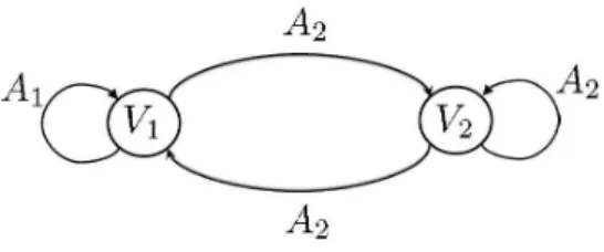
Example 1: The graph depicted in Figure 2 (a graph with m = 2 labels) is path-complete: one can check that every word can be readas a pathon this graph. As a consequence, the following set ofLMIs
Fig. 2. A graph corresponding to the LMIsin (8). The graph is path-complete, and as a consequence anyswitched systemfor which these LMIs have a solution is stable.
AT r 1 P1A1 ≺ P1 AT r1 P1A1 ≺ P2 AT r2 P2A2 ≺ P1 AT r 2 P2A2 ≺ P2 P1, P2 ≻ 0. (8)
Unlike this simple example, the structure of path-complete graphs can be quite complicated, leading to rather nontrivial sets of LMIs that imply stability; see the examples in [AJPR14] such as Proposition 3.6.
In this note, we mainly investigate the converse of Theorem 2 and answer the question “Are there other sets of Lyapunov inequalitieswhich do not correspond to path-complete graphs but are sufficient conditions for stability?” The answer is negative.Thus, path-completeness fully characterizes the set of all stability-proving Lyapunov inequalities. By Remark 1, this also leads to a complete characterization of all valid inequalities for approximation of the joint spectral radius.
To this purpose, in the next section we show that for any non-path-complete graph, there exists a set of matrices which is not stable, but yet makes the corresponding Lyapunov inequalities feasible.This is not a trivial task a priori, because we need to construct a counterexample without knowing the graph
explicitly, but just with the information that it is not path-complete.With this information alone we need to provide two things: (i) a set of matrices that are unstable, and (ii) a set of Lyapunov functionsVi such
that the Lyapunov inequalities associated to the edges (with the matrices found in (i)) are feasible.
III. THE MAIN RESULT (NECESSITY OF PATH-COMPLETENESS)
A. The construction
As stated just above, we want to prove that if a graph is not path-complete, it does not provide a valid criterion for stability, meaning that there must exist an unstable set of matrices that satisfies the
Fig. 3. Graphical representation of the construction of the set of matricesΣw for w = 2212111 : the edges with label 1
represent the matrix A1 (i.e. A1 is the adjacency matrix of the subgraph with edges labeled with a “1”), and the edges with
label2 represent the matrix A2.
corresponding Lyapunov inequalities. Our goal in this subsection is to describe a simple construction that will allow us to build such a set. If a graph is not path-complete, there is a certain word w which
cannot be“read”on the graph. We propose a simple construction of a set of matrices with the following property: any long product of these matrices which is not equal to the zero matrix must contain the product Aw.
Definition 3: Let w ∈ {1, 2, . . . , r}∗ be a word on an alphabet of r characters and let n = |w| + 1.
Wedenote by Σw the set ofn × n{0, 1}-matrices2 {A1, A2, . . . , Ar} such that the (i, j) entry of Al is equal to one if and only if
• j = i + 1, and wi = l, for 1 ≤ i ≤ n − 1, or
• (i, j) = (n, 1) and l = 1.
In other words,Σw is the only set of binary matrices whose sum is the adjacency matrix of the cycle on n nodes, and such that for all i ∈ {1, . . . , n − 1}, the ith edge of this cycle is in the graph corresponding
to Awi, the last edge being in the graph corresponding to A1. Figure 3 provides a visual representation
of the setΣw.
The following lemma characterizes the main property of our construction Aw in a straightforward fashion.
Lemma 1: Any nonzero product in Σ2nw containsAw as a subproduct.
Proof:Recall that the matrices inΣw are adjacency matrices of a subgraph of the cycle on n nodes.
Hence, a nonzero product corresponds to a path in this graph. A path of length more thann must contain
2
a cycle. Since there is only one cycle in this graph, this cycle is the whole graph itself. Finally, a path of length2n must contain a cycle starting at node 1 (i.e., the node corresponding to the beginning of the
wordw). Hence, this product contains Aw.
B. The proof
Let us consider an arbitrary non-path-complete graph. From this graph, we will first construct a set of matrices which is not stable. Then we will prove that the corresponding inequalities, as given by our automatic recipe thatassociates graphs with Lyapunov inequalities via Figure 1, admit a solution.For this purpose, we will take our Lyapunov functions to be quadratic functions (though a similar construction is possible for other classes of Lyapunov functions). Thus, we will have to find a solution (that is, a set of
positive definitematricesPi) to particular sets of LMIs. It turns out that for our purposes, we can restrict
our attention to diagonal matrices P = diag(p), wherep ∈ Rn is a positive vector. For these matrices, the corresponding Lyapunov functions satisfy3:
Vp(x) = n X
i=1
p(i)x2i. (9)
The following proposition provides an easy way to express Lyapunov inequalities among diagonal quadratic forms. It will allow us to write the Lyapunov inequalities in terms of entrywise vector inequal-ities.
Proposition 1: Let p, p′ ∈ Rn
++ (i.e. p, p′ are positive vectors), and A ∈ {0, 1}n×n be matrices with
not more than one nonzero entry in every row and every column. Then, we have
∀x ∈ Rn, Vp′(AT rx) < Vp(x) ⇐⇒ Ap′< p, (10)
where the vector inequalities are to be understood componentwise, and the Lyapunov functions Vp and
Vp′ are as in Equation (9).
Proof:⇒: For an arbitrary index 1 ≤ l′ ≤ n, consider the l′th row in the right-hand side inequality.
If the l′th row of A is equal to the zero vector, then the inequality is obvious. If not, take the index 1 ≤ l ≤ n such that Al′,l= 1, and fix x = el′,that is, thel′th canonical basis vector.Then the left-hand
side of (10) becomes
p′(l) < p(l′),
which is exactly thel′th row of the entrywise inequality we wish to prove.
⇐: Writing P′ = diag(p′), we have: AP′AT r = A X l p′(l)eleT rl ! AT r (11) = X l p′(l)(Ael)(Ael)T r ≺ X l′ p(l′)el′eT rl′ = P,
which is equivalent to the left-hand side of (10).
In the previous subsection, we have shown how to build, for a particular non path-complete graph, a set of matrices, which is clearly not stable. In the above proposition, we have shown that, for such matrices (with not more than one one-entry in every row and every column), the Lyapunov inequalities translate into simple constraints (namely, entrywise vector inequalities), provided that the quadratic Lyapunov functions Pi have the simple form of Equation (9). Now, we put all these pieces together: we show
how to construct such Lyapunov functions, and use our characterization (10) in order to prove that these functions satisfy the Lyapunov inequalities.
Theorem 3: A set of quadratic Lyapunov inequalities is a sufficient condition for stability if and only if the corresponding graph is path-complete.
Proof: The if part is exactly Theorem 2. We now prove the converse: for any non path-complete graph, we constructively provide a set of matrices that satisfies the corresponding Lyapunov inequalities (with Lyapunov functions of the form (9)), but which is not stable.Our proof works in three steps: first, for a given graph which is not path-complete, we show how to build a particular unstable set of matrices. Then, we compute a set of solutions pi for our Lyapunov inequalities, and finally, we prove that these pi are indeed valid solutions, for the particular matrices we have built.
1. The counterexample
For a given graphG which is not path-complete, there is a word w that cannot be read as a subword of
a sequence of labels on a path in this graph. We use the construction above with the particular wordw.
We show below that the set of Lyapunov inequalities corresponding to G admits a solution for the set
of matrices (see Definition 3)
ΣT rw = {AT r: A ∈ Σw}.
Actually, we show that for these matrices, there is in fact a solution within the restricted family of diagonal quadratic Lyapunov functions defined in (9). Since ΣT rw is not stable by construction, this will
conclude the proof.
2. Explicit solution of the Lyapunov inequalities
We have to construct a vectorpi defining a norm for each node of the graph G. In order to do this, we
construct an auxiliary graph G′(V′, E′) from the graph G. The nodes of G′ are the couples (N is the
number of nodes in G and n is the dimension of the matrices in ΣT rw ):
V′ = {(i, l) : 1 ≤ i ≤ N, 1 ≤ l ≤ n}
(that is, each node represents a particular entry of a particular Lyapunov functionpi). There is an edge
in E′ from(i, l) to (j, l′) if and only if
1) there is an edge from i to j in G with label Ak (where Ak can represent a single matrix, or a
product of matrices),
2) the corresponding matrix Ak(Ak is a matrix inΣw, or possibly a product of such matrices) is such
that
(Ak)l,l′ = 1. (12)
We give the labelAk to this edge in G′.
We claim that G′ is acyclic. Indeed, by (12), a cycle (i, l) → · · · → (i, l) in G′ describes a product
of matrices in Σw such thatAl,l = 1. (We can build this product by following the labels of the cycle.)
Now, take a nonzero product of length2n by following this cycle (several times, if needed). By Lemma
1, any long enough nonzero product of matrices inΣw contains the productAw; and thus there is a path
with label w in G′.
Now, by item 1. in our construction ofG′, any such path in G′ corresponds to a path inG with the same
sequence of labels w, a contradiction; and this proves the claim.
Let us constructG′ = (V′, E′) as above. It is well known that the nodes of an acyclic graph admit a
renumbering
s : V → {1, . . . , |V |} : v → s(v)
such that there can be a path from v to v′ only if s(v) > s(v′) (see [Kah62]). This numbering finally
allows us to define our nonnegative vectors pi in the following way:
pi(l) := s((i, l)).
3. Proof that the solution {pi} is valid
We have to show that for every edge i → j of G = (V, E) with label Ak, the following holds ∀x, Vpj(A
T r
By Proposition 1 above, we can instead show that
Akpj < pi. (13)
If (Akpj)l = 0, then (13) obviously holds at its lth component. If (Akpj)l 6= 0, we have a particular
index l′ such that(Ak)l,l′ = 1, and
(Akpj)l= (pj)l′.
Now, it turns out that indeed
(pj)l′ < (pi)l.
This is because(Ak)l,l′ = 1, together with (i, j) ∈ E implies (by our construction) that there is an edge
((i, l) → (j, l′)) ∈ E′. Thus, (pj)l′ < (pi)l, which gives the required Inequality (13), and the proof is
complete.
Example 2: The graph represented in Figure 4 is not path-complete:one can easily check for instance that the wordA1A2A1 cannot be read as a subword of a path in the graph. As a consequence, the set of
LMIs in (14) is not a valid condition for stability, even though it is very much similar to (8).
AT r1 P1A1 ≺ P1 AT r 2 P1A2 ≺ P2 AT r 2 P2A2 ≺ P1 AT r2 P2A2 ≺ P2 P1, P2 ≻ 0. (14)
As an example, one can check that the set of matrices
Σ = −0.7 0.3 0.4 0.4 0 0.8 −0.7 0.5 0.7 , −0.3 −0.95 0 0.4 0.5 0.8 −0.6 0 0.2
makes (14) feasible, even though this set is unstable. Indeed,
ρ(Σ) ≥ ρ(A1A2A1)1/3 = 1.01 . . .
It is not surprising that this unstable product precisely corresponds to a “missing” word in the language generated by the automaton in Figure 4.
Fig. 4. The graph corresponding to the LMIs in (14). The graph is not path-complete: one can easily check for instance that the word A1A2A1 cannot be read as a path in the graph.
C. PSPACE-completeness of the recognizability problem
Our results imply that it is PSPACE-complete to recognize sets of LMIs that are valid stability criteria.
PSPACE-complete problems are a well-known class of problems, harder than NP-complete, see [GJ90] for details.
Theorem 4: Given a set of quadratic Lyapunov inequalities, it is PSPACE-completeto decide whether they constitute a valid stability criterion.
Proof: Our proof works by reduction from thefull language problem. In thefull language problem, one is given a finite state automaton on a certain alphabet Σ, and it is asked whether the
language that it accepts is the language Σ∗ of all the possible words. It is well known that the full language problem is PSPACE-complete ([GJ90]).
A labeled graph corresponds in a straightforward way to a finite state automaton. However, the concept of automaton is slighlty more general, in that they include in their definition a set of starting states, and terminating states, so that each path certifying that a particular word belongs to the language must start (resp. end) in a starting (resp. terminating) state. Thus, in order to reduce the full language problemto the question of recognizing whether a graph is path-complete, we must be able to transform the automaton into a new one for which all the states are starting and accepting. For this purpose, we will need to introduce a new fake characterf in the alphabet.
So, let us be given an arbitrary automaton. We then connect all accepting nodes to all starting nodes, with an edge labeled with the new characterf. Now, we make all the nodes starting and accepting, and
we ask whether all the words in our new alphabetΣ ∪ {f } are accepted in our new automaton, that is, if the obtained graph is path-complete.
If all words can be read on the graph, then in particular,all words starting and ending with the character
generates all the words on the initial alphabet.
Conversely, if the initial automaton generates all the words on the initial alphabet, by decomposing an arbitrary word on the new alphabet as w = w1f w2f . . . f, we see that we can generate all the words
on the new alphabetΣ ∪ {f }. In other words, the new graph is path-complete if and only if the initial automaton was accepting all the words on Σ∗. The proof is complete.
IV. INVARIANT SETS ANDPATH-COMPLETE GRAPHS
Recall that Theorem 2 states that Lyapunov inequalities associated with any path-complete graph imply stability of the switched system in (1). The proof of this theorem, as it appears in [AJPR11], [AJPR14], does not give rise to an explicit common Lyapunov function for system (1). In other words, if the conditions of Theorem 2 are satisfied, then we know that system (1) isstable, but it is not clear how to construct an invariant set for its trajectories. The question hence naturally arises (and has been repeatedly brought up to us in presentations of our previous work) as to whether one can construct a single common Lyapunov functionW (i.e., one that satisfies W (Aix) < W (x), ∀x 6= 0, ∀i ∈ {1, . . . , m}) by combining
the Lyapunov functionsVi assigned to each node of the graph. This is the question that we address in this
section.4 We start with a simple proposition that establishes a “bi-invariance” property, showing that a
path-complete graph Lyapunov function implies existence of two sets in the state space with the property that points in one never leave the other.
Proposition 2: Consider any path-complete graph G with edges labeled by
{A1, . . . , Am} and suppose there exist Lyapunov functions V1, . . . , Vk, one per node of G, that satisfy
the inequalities imposed by the edges. Then, for all α ≥ 0, and for all finite products Aσs· · · Aσ1, if
¯
x ∈ ∩l=1,...,k{x| Vl(x) ≤ α}, then
Aσs· · · Aσ1x ∈ ∪l=1,...,k¯ {x| Vl(x) ≤ α}.
Proof: This is an obvious consequence of the definition of Lyapunov inequalities.
Knowing that points in the intersection of the level sets of Vi never leave their union may be good enough for some applications. Nevertheless, one may be interested in having a true invariant set. This is achieved in the following construction, which is completely explicit but comes at the price of increasing the complexity of the set.
4
For the purposes of this section, we assume that the labels on our edges are matrix products of length one, though the extension to the general case is straightforward.
Theorem 5: For a finite set of matricesA = {A1, . . . , Am} and a scalar γ, let Aγ := {γA1, . . . , γAm}.
Consider any path-complete graph G with edges labeled by the matrices in Aγ. Suppose there exist Lyapunov functions V1, . . . , Vk, one per node of G, that satisfy the inequalities imposed by the edges
of G with γ > 1. Then one can explicitly write down (from the Lyapunov functions V1, . . . , Vk and
matrices A1, . . . , Am) a single Lyapunov function W (x), which is a sum of pointwise maximum of
quadratic functions, and satisfies
W (Aix) < W (x), ∀i ∈ {1, . . . , m}, ∀x 6= 0. (15)
Proof: Since the Lyapunov functions Vi are positive definite and continuous, there exist positive
scalarsαi, βi, such that
αi ≤ Vi(x) ≤ βi,
for allx with ||x|| = 1 and for i = 1, . . . , k. The scalars αi, βi can be explicitly computed by minimizing
and maximizing Vi over the unit sphere. (In fact, one can show that a finite upper bound on βi and a
finite lower bound onαi can be found by solving two polynomially-sized sum of squares programs; such
bounds would be sufficient for our purposes.) Let
ξ := max
i,j∈{1,...,k} βi αj
. (16)
In [AJPR14] (Equation 2.4 and below), the following upper bound is proven on the spectral norm of an arbitrary product of length s:
||Aσs· · · Aσ1|| ≤ ξ 1 dm 1
γs, (17)
where dm is the maximum degree of homogeneity of the functions Vi. Let r be the smallest integer s
that makes the right hand side of the previous inequality less than one. Note that r can be explicitly
computed from γ and V1, . . . , Vk, once the Lyapunov inequalities are solved. Let E(x) := ||x||2. Then
we claim that
W (x) = E(x) + max
i∈{1,...,m}E(Aix) +i,j∈{1,...,m}max 2E(AiAjx)
+ · · · + max
satisfies (15). Indeed, for any l ∈ {1, . . . , m} and any x 6= 0,
W (Alx) = E(Alx) + maxi∈{1,...,m}E(AiAlx)
+ · · · + maxσ∈{1,...,m}r−1E(Aσr−1· · · Aσ1Alx)
≤ maxi∈{1,...,m}E(Aix) + · · · + maxσ∈{1,...,m}rE(Aσr· · · Aσ
1x)
= W (x) − E(x) + maxσ∈{1,...,m}rE(Aσr· · · Aσ 1x)
< W (x),
where the last inequality follows from (17) and the definition of r.
Note that we did not assume in the theorem above that the Lyapunov functions are quadratic, and indeed the proof works for general Lyapunov functions as considered in this paper.
V. CONCLUSIONS
There has been a surge of research activity in the last fifteen years to derive stability conditions for switched systems. In this work, we took this research directionone step further. We showed that all stability-proving Lyapunov inequalities within a broad and canonical family can be understood by a single language-theoretic framework, namely that of path-complete graphs. Our work also showed that one can always use the Lyapunov functions associated with the nodes of a path-complete graph to construct an invariant set for the switched system.As explained before, our results are not only relevant for proving stability of switched systems, but also for the goalof approximating the joint spectral radius of a set of matrices.
A corollary of our main result is that testing whether a set of equations provides a valid sufficient condition for stability is PSPACE-complete, and hence intractable in general. In practice, however, one can choose to work with a fixed set of path-complete graphs whose path-completeness has been certified a priori. In view of this, we believe it is worthwhile to systematically compare the performance of different path-complete graphs, either with respect to all input matrices {Ai}, or those who may have a specific
structure.We leave that for further work.
This note leaves open many questions, on which we are actively working: For example, our main result is devoted to LMI Lyapunov criteria. Intuitively, one might expect that it would be valid for much more general Lyapunov functions. However, our proof uses algebraic properties of these functions, so that it is not clear how to generalize it to more general families.
VI. ACKNOWLEDGEMENT
We would like to thank Marie-Pierre B´eal, Vincent Blondel, and Julien Cassaigne for helpful discussions leading to Theorem 4.
REFERENCES
[Ahm08] A. A. Ahmadi. Non-monotonic Lyapunov functions for stability of nonlinear and switched systems: theory and computation, 2008. Master’s Thesis, Massachusetts Institute of Technology. Available from
http://dspace.mit.edu/handle/1721.1/44206.
[AJPR11] A. A. Ahmadi, R. M. Jungers, P. A. Parrilo, and M. Roozbehani. Analysis of the joint spectral radius via lyapunov functions on path-complete graphs. In Hybrid Systems: Computation and Control (HSCC’11), Chicago, 2011. [AJPR12] A. A. Ahmadi, R. M. Jungers, P. A. Parrilo, and M. Roozbehani. When is a set of LMIs a sufficient condition
for stability? In Proc. of ROCOND12, Aalborg, 2012. Arxiv Preprint http://arxiv.org/abs/1201.3227.
[AJPR14] A. A. Ahmadi, R. M Jungers, P. A. Parrilo, and M. Roozbehani. Joint spectral radius and path-complete graph Lyapunov functions. SIAM Journal on Control and Optimization, 52(1):687–717, 2014.
[AS98] T. Ando and M.-H. Shih. Simultaneous contractibility. SIAM Journal on Matrix Analysis and Applications, 19(2):487–498, 1998.
[BFT03] P.-A. Bliman and G. Ferrari-Trecate. Stability analysis of discrete-time switched systems through Lyapunov functions with nonminimal state. In IFAC Conference on the Analysis and Design of Hybrid Systems, 2003. [Bra98] M. S. Branicky. Multiple Lyapunov functions and other analysis tools for switched and hybrid systems. IEEE
Transactions on Automatic Control, 43(4):475–482, 1998.
[CCJ08] V. Crespi, G. Cybenko, and G. Jiang. The theory of trackability with applications to sensor networks. ACM
Transactions on Sensor Networks, 4(3):1–42, 2008.
[DB01] J. Daafouz and J. Bernussou. Parameter dependent Lyapunov functions for discrete time systems with time varying parametric uncertainties. Systems and Control Letters, 43(5):355–359, 2001.
[GJ90] M. R. Garey and D. S. Johnson. Computers and Intractability; A Guide to the Theory of NP-Completeness. W. H. Freeman & Co., New York, NY, 1990.
[GPV12] A. Garulli, S. Paoletti, and A. Vicino. A survey on switched and piecewise affine system identification. IFAC
Proceedings Volumes, 45(16):344–355, 2012.
[GTHL06] R. Goebel, A. R. Teel, T. Hu, and Z. Lin. Conjugate convex Lyapunov functions for dual linear differential inclusions. IEEE Transactions on Automatic Control, 51(4):661–666, 2006.
[GZ08] N. Guglielmi and M. Zennaro. An algorithm for finding extremal polytope norms of matrix families. Linear
Algebra and its Applications, 428:2265–2282, 2008.
[HVMCB11] E. Hernandez-Varga, R. Middleton, P. Colaneri, and F. Blanchini. Discrete-time control for switched positive systems with application to mitigating viral escape. International Journal of Robust and Nonlinear Control, 21:1093–1111, 2011.
[JR98] M. Johansson and A. Rantzer. Computation of piecewise quadratic Lyapunov functions for hybrid systems. IEEE
Transactions on Automatic Control, 43(4):555–559, 1998.
[Jun09] R. M. Jungers. The joint spectral radius, theory and applications. In Lecture Notes in Control and Information
[Kah62] A. B. Kahn. Topological sorting of large networks. Communications of the ACM, 5:558–562, 1962.
[LD06] J. W. Lee and G. E. Dullerud. Uniform stabilization of discrete-time switched and Markovian jump linear systems.
Automatica, 42(2):205–218, 2006.
[MM11] T. Monovich and M. Margaliot. Analysis of discrete-time linear switched systems: a variational approach. SIAM
Journal on Control and Optimization, 49:808–829, 2011.
[PJ08] P. A. Parrilo and A. Jadbabaie. Approximation of the joint spectral radius using sum of squares. Linear Algebra
and its Applications, 428(10):2385–2402, 2008.
[PJB10] V. Yu. Protasov, R. M. Jungers, and V. D. Blondel. Joint spectral characteristics of matrices: a conic programming approach. SIAM Journal on Matrix Analysis and Applications, 31(4):2146–2162, 2010.
[RMFF08] M. Roozbehani, A. Megretski, E. Frazzoli, and E. Feron. Distributed Lyapunov functions in analysis of graph models of software. Springer Lecture Notes in Computer Science, 4981:443–456, 2008.
[TB97] J. N. Tsitsiklis and V.D. Blondel. The Lyapunov exponent and joint spectral radius of pairs of matrices are hard-when not impossible- to compute and to approximate. Mathematics of Control, Signals, and Systems, 10:31–40, 1997.
[WDA+
09] G. Weiss, A. D’Innocenzo, R. Alur, K. Johansson, and G. J. Pappas. Robust stability of multi-hop control networks. In Proc. of CDC 2009, pages 2210–2215, 2009.