MIT Joint Program on the Science and Policy of Global Change
combines cutting-edge scientific research with independent policy analysis to provide a solid foundation for the public and private decisions needed to mitigate and adapt to unavoidable global environmental changes. Being data-driven, the Joint Program uses extensive Earth system and economic data and models to produce quantitative analysis and predictions of the risks of climate change and the challenges of limiting human influence on the environment— essential knowledge for the international dialogue toward a global response to climate change.
To this end, the Joint Program brings together an interdisciplinary group from two established MIT research centers: the Center for Global Change Science (CGCS) and the Center for Energy and Environmental Policy Research (CEEPR). These two centers—along with collaborators from the Marine Biology Laboratory (MBL) at
Woods Hole and short- and long-term visitors—provide the united vision needed to solve global challenges.
At the heart of much of the program’s work lies MIT’s Integrated Global System Model. Through this integrated model, the program seeks to discover new interactions among natural and human climate system components; objectively assess uncertainty in economic and climate projections; critically and quantitatively analyze environmental management and policy proposals; understand complex connections among the many forces that will shape our future; and improve methods to model, monitor and verify greenhouse gas emissions and climatic impacts.
This reprint is intended to communicate research results and improve public understanding of global environment and energy challenges, thereby contributing to informed debate about climate change and the economic and social implications of policy alternatives.
—Ronald G. Prinn and John M. Reilly, Joint Program Co-Directors
MIT Joint Program on the Science and Policy
of Global Change Massachusetts Institute of Technology 77 Massachusetts Ave., E19-411 Cambridge MA 02139-4307 (USA)
T (617) 253-7492 F (617) 253-9845 [email protected]
http://globalchange.mit.edu/
June 2017
Can Tariffs be Used to Enforce
Paris Climate Commitments?
Can Tariffs be Used to Enforce Paris Climate
Commitments?
niven Winchester1,2
Abstract: We evaluate the potential for using border carbon adjustments (BCAs) and welfare-maximizing tariffs to compel non-compliant countries to meet emissions reduction targets pledged under the Paris Climate Agreement. Our analysis employs a numerical economy-wide model with energy sector detail and, given recent actions by the new US administration, considers BCAs on US exports. We find that BCAs result in small reductions in US emissions and welfare. Consequently, the US is better off when it does not restrict emissions and faces BCAs on its exports than when it implements policies consistent with the Paris Agreement. However, targeted welfare-maximizing tariffs could inflict greater cost on the US than if it complied with its pledged emissions reductions. We conclude that BCAs are an ineffective enforcement mechanism but carefully chosen tariffs could be a mechanism to enforce the Paris Agreement.
1 Joint Program on the Science and Policy of Global Change, Massachusetts Institute of Technology, Cambridge, MA 02139, USA. Email: [email protected].
2 The author gratefully acknowledges helpful comments and suggestions from Rudy Colacicco, Martin Richardson, John Reilly and participants at the 12th Australasian Trade Workshop.
1. INTRODUCTION ...2
2. METHODS ...3
2.1 MODeLInG FRAMeWORK ...3
2.2 SCenARIOS ...5
2.3 BORDeR CARBOn ADJuSTMenTS & eMBODIeD CO2 eMISSIOnS ...6
3. RESULTS ...6
3.1 SeCTORAL eMISSIOnS InTenSITIeS & uS eXPORTS ...6
3.2 PARIS PLeDGeS & BORDeR CARBOn ADJuSTMenTS ... 7
3.3 A TARIFF WAR ... 10
4. CONCLUSIONS ...11
1. Introduction
At the 2015 Paris Climate Conference—the 21st
Confer-ence of the Parties (COP21) under the United Nations Framework Convention on Climate Change (UNFCC)— representatives from 195 countries set out an agreement to mitigate greenhouse gas (GHG) emissions. The frame-work required countries representing at least 55% of global GHG emissions to sign up to the agreement for it to take force. This occurred in October 2016 and the Par-is Agreement was formally ratified on November 4, 2016. Nations that are parties to the agreement are required to submit National Determined Contributions (NDCs) that outline future reductions in GHG emissions out to 2030. The US, under the Obama Administration, submitted its NDC on September 3, 2016. This document stated that the US would reduce economy-wide GHG emissions by 26–28 percent below its 2005 level by 2025. However, this pledge, like all NDCs, is not binding under international law and a nation can back out of the deal with four years notice by withdrawing from the agreement (Stutter, 2017) or in one year by leaving the UNFCC (Mathiesen, 2016). Following the 2016 US presidential election, the future involvement of the US in the global accord is uncertain. Although the carbon pricing scheme recently proposed by an eminent group of Republicans (Baker et al., 2017) and Secretary of State Ross Tillerson’s statement that the US should remain a party to the Paris Agreement (DiChristopher, 2017) indicate that the US may meet its NDC goal, other signs from the Trump Administration paint a different picture. In the lead up to the 2016 elec-tion, Donald Trump vowed to remove the US from the Paris Agreement (Stutter, 2017) and in 2012 Trump post-ed on Twitter, ‘The concept of global warming was creat-ed by and for the Chinese in order to make US manufac-turing non-competitive’ (Wong, 2016). Trump’s actions since taking office have been consistent with his pre-elec-tion view on climate change. Significantly, Trump signed an executive order on March 28, 2017 that initiated a review of the Clean Power Plan—an Obama administra-tion policy that aims to reduce carbon dioxide emission from electricity generation—and rescinded the morato-rium on coal mining on US federal lands (Merica, 2017). Other senior Republicans are also dismissive about climate change. For example, Environmental Protection Agency (EPA) Chief Scott Pruitt stated that carbon dioxide (CO2)
is not a primary contributor to global warming and that the Paris Agreement is a ‘bad deal’ (DiChristopher, 2017). Additionally, House of Representatives Speaker Paul Ryan has stated that ‘the Paris climate deal would be disastrous for the American economy’ (Doyle and Rampton, 2016). The 2016 presidential election has also resulted in a change in US trade policy, from actively seeking trade liberaliza-tion to a more protecliberaliza-tionist stance. Notably, shortly after
his inauguration, President Trump withdrew the US from negotiations for the Trans-Pacific Partnership Agreement. The White House also plans to renegotiate the North American Free Trade Agreement and the President has stated that the US will terminate the agreement if a ‘fair’ deal is not reached (Liptak and Merica, 2017). On April 24, 2017 he announced plans to impose tariffs of up 24% on Canadian lumber entering the US (Gillespie, 2017). In this paper, we evaluate the role of border carbon ad-justments (BCAs) and welfare-maximizing tariffs as a mechanism to persuade a non-compliant country to re-duce GHG emissions. BCAs—tariffs on embodied car-bon emissions imposed by countries with climate poli-cies on imports from countries without them—have been proposed in policy circles. For example, the directive for the EU Emissions Trading System includes provisions for BCAs, and the American Clean Energy and Security Act of 2009 (US Congress, 2009), which was passed by the House of Representatives but died in the Senate, includ-ed import requirements analogous to a tariff on embod-ied carbon emissions (Winchester et al., 2011).
Most previous studies of BCAs have focused on the im-pact of BCAs on emissions and consider tariffs imposed by a group of developed countries on imports from other nations (e.g., Felder and Rutherford 1993; Demailly and Quirion 2008; Ponssard and Walker 2008; Mattoo et al. 2009; Burniauxet et al. 2010; Winchester et al., 2011; Win-chester, 2012; and Sakai and Barrett, 2016). Babiker and Rutherford (2005) consider a menu of border measures (e.g., border carbon adjustments and rebates on exports) imposed by countries parties to the Kyoto agreement on imports from other countries and derive the Nash equi-librium over trade instruments. In reviewing the BCA literature, Böhringer et al. (2012) note that carbon tariffs shift some cost of reducing emissions from regions that restrict emissions to those that do not. We build on this literature by evaluating the role of BCAs and other trade measures as an enforcement mechanism to persuade a non-compliant country to reduce GHG emissions. Motivated by recent actions by the US that would make it appear unlikely it would live up to its Paris commitment, our analysis considers a case where all regions except the US implement polices to reduce emissions and US exports face BCAs. Using a global multi-sectoral, multi-region economy-wide model with energy sector detail, we quan-tify outcomes under this case and compare them to a case where all regions meet their Paris pledges. We also com-pare the impact of BCAs to the Nash equilibrium of a ‘tariff war’ where countries impose welfare maximizing tariffs.1
1 Our quantification of tariff outcomes does not consider the legal aspects of these measures under international treaties. See Kemp (2016) for a discussion of these issues.
This paper has three further sections. Section 2 describes the structure and data sources for our economy-wide model and the scenarios implemented in our analysis. Our results are presented and discussed in Section 3. Section 4 concludes.
2. Methods
2.1 Modeling Framework
Our analysis employs an economy-model with a detailed representation of energy production that builds on the ‘GTAP-Energy in GAMS’ model (Rutherford and Palt-sev, 2000). The model is a static, multi-sector, multi-re-gion applied general equilibrium model of the global economy that links economic activity to energy produc-tion and CO2 emissions from the combustion of fossil
fuels. Regions in the model are interconnected via bilat-eral international trade flows and sectors are linked by purchases of intermediate inputs.
In each region and sector, there is a representative firm that produces output by hiring primary factors and pur-chasing intermediate inputs from other firms. There is also a representative agent in each region that derives income from selling factor services and an exogenous net international transfer that reflects the current ac-count balance. A government sector is not explicitly modelled, but taxes and subsidies on transactions are represented, and government purchases are included in
household consumption in each region. Net fiscal deficits and, where applicable, revenue from the sale of emission permits are passed to consumers as (implicit) lump sum transfers. Although the model is static, investment is in-cluded as a proxy for future consumption and is a fixed proportion of expenditure by each regional household. Sectors, regions and primary factors included in the model are listed in Table 1. The model represents three sectors related to the extraction of fossil fuels (Coal, Crude oil, Natural gas) and two sectors that process these fuels into secondary energy (Refined oil and Electricity). Fossil fuels are also used directly by other sectors and re-gional households. The representation of manufacturing includes four sectors that use energy intensively (Chem-ical, rubber & plastic products; Non-metallic minerals; Iron and steel; and Non-ferrous metals) and seven oth-er manufacturing sectors (Food processing; Fabricated metal products, Textiles, clothing & footwear; Transpor-tation equipment; Electronic equipment; Other machin-ery and equipment; and Other manufacturing). Agricul-tural activities and services are each included in separate aggregated sectors.
The model represents the US and seven regions that ac-count for a high share of US exports or/and have set out ambitious plans to reduce GHG emissions. Most of these regions are individual countries (e.g., Canada, Mexico, and China), but some regions include an aggregation of na-Table 1. Model aggregation.
Sectors Regions
agr Agriculture usa USA
Cru Crude oil anz Australia & New Zealand
Oil Refined oil products can Canada
Col Coal chn China
Gas Natural gas jpn Japan
ele Electricity eur European Union & EFTA
crp Chemical, rubber & plastic products mex Mexico
nmm Non-metallic minerals kor South Korea
is Iron and Steel row Rest of World
Nfm Non-ferrous metals
Fmp Fabricated metals products Primary factors
Fod Food processing cap Capital
Tcf Textiles, clothing & footwear lab Labor
Trn Transportation equipment rcr Crude oil resources
Eeq Electronic equipment rco Coal resources
Ome Other machinery & equipment rga Natural gas resources
Omf Other manufacturing
tions (Australia & New Zealand and the European Union & European Free Trade Area, EFTA). Remaining countries are included in a composite ‘Rest of World’ region. Brazil, Russia and India are not represented as separate regions as several studies estimate that 2030 emissions consistent with NDC pledges are close to or above BAU emissions— see, for example, Fawcett et al. (2015), Aldy et al. (2016), Vandyck et al. (2016) and Jacoby et al. (2017). Primary factors in the model include capital, labor, and primary resources for the extraction of each fossil fuel.
For computational reasons, we also simulate some scenarios using a more aggregated version of the model (see Section 2.2). This aggregation represents two regions, seven sec-tors, and the primary factors listed in Table 1. The regional aggregation representing the US and all other countries are included in a composite region that we label the ‘Coalition’. Sectors in the more-aggregate version of the model include the five energy sectors in Table 1 (Coal, Crude oil, Natural gas, Refined oil, and Electricity), services, and ‘Other in-dustry’, a composite of the remaining sectors.
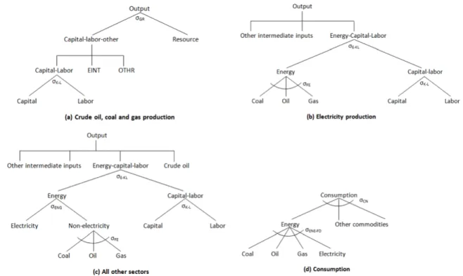
Production in each sector is represented by a multi-level nest of constant elasticity of substitution (CES) functions. Production structures are outlined in panels (a), (b) and (c) of Figure 1. Fossil fuel commodities are produced by a CES aggregate of a sector-specific resource and a com-posite of capital, labor and intermediate inputs. Other sec-tors combine intermediate inputs, capital and labor. Final consumption in each region is also represented by nested a CES function, as outlined in panel (d). Use of Coal, Re-fined oil, or Natural gas, either as intermediate inputs or in
final consumption, result in the release of CO2 emissions
in fixed proportions with the use of each fuel.
Features of the model that have a large influence on the cost of abating emissions include: (1) substitution among different forms of energy in production and final con-sumption, (2) substitution between aggregate energy and capital-labor in production, and (3) substitution between aggregate energy and other goods in final consumption. The production structure and elasticity values that, in tandem with input cost shares, govern these substitution possibilities are detailed in the notes to Figure 1 and are guided by those used in the MIT Economic Projection and Policy Analysis (EPPA) model (Paltsev et al., 2005; Chen et al., 2016). To account for the increased pene-tration of low-carbon generation sources under a carbon price, we set the elasticity of substitution between energy and capital-labor in electricity generation equal to 0.85, compared to 0.6 in Paltsev et al. (2005). This higher elas-ticity of substitution increases the scope for producing electricity with less fuel and more capital in response to rising fuel costs. Implied marginal abatement cost curves in the model are increasing convex functions of the quantity of emissions abated.
International trade in goods and services follows the ‘Armington approach’ that assumes that goods are differ-entiated by country of origin (Armington, 1969). Specif-ically, for each region and commodity, imports are com-bined using a CES function that aggregates goods from different regions, and aggregate imports are and domestic production are combined using a further CES function.
This two-level CES next produces an ‘Armington’ supply for each commodity, which is purchased by firms and households and is a composite of domestic and import-ed varieties. Values for elasticities of substitution in the trade specification are sourced from Hertel et al. (2007). Turning to closure, factor prices are endogenous and there is full employment; factors are immobile internationally, but capital and labor are mobile across sectors; and each re-gion maintains a constant current account surplus/deficit. The model is calibrated using version 9 of the Global Trade Analysis Project (GTAP) database (Aguiar et al., 2016) and the GTAP-Power database (Peters, 2016). These databases include economic data and CO2 emissions from the
com-bustion of fossil fuels for 140 regions and 68 sectors, which we aggregate to the elements in Table 1 using tools provid-ed by Lanz and Rutherford (2016). The database provides a snapshot of the global economy in 2011.
The model is formulated and solved as a mixed comple-mentarity problem using the Mathematical Program-ming Subsystem for General Equilibrium (MPSGE) described by Rutherford (1995) and the Generalized Al-gebraic Modeling System (GAMS) mathematical mod-eling language (Rosenthal, 2012) with the PATH solver (Dirkse and Ferris, 1995).
2.2 Scenarios
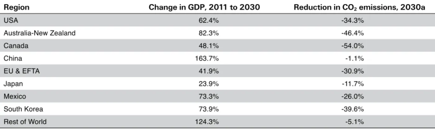
To focus the analysis on the period when NDCs will have the largest impact, our scenarios estimate outcomes in 2030. As the model is calibrated to 2011 data, we imple-ment a forward calibration simulation to generate a 2030 ‘business as usual’ (BAU) case. Our BAU projection sim-ulates autonomous energy efficiency improvements and endogenous increases in total factor productivity to tar-get estimates of GDP in each region in 2030. We impose autonomous energy efficiency improvements of 1% per year in fossil fuel use, and a 0.03% annual efficient im-provement in electricity use. We source estimates of 2030 GDP from the OECD (2014) and report proportional changes in GDP between 2011 and 2030 imposed in the
BAU simulation in Table 2. In the policy scenarios, to-tal factor productivity parameters are set equal to values derived in the BAU simulation and GDP is endogenous. Jacoby et al. (2017) estimate emissions from the combus-tion of fossil fuels under a reference (no climate policies) case and a scenario when regions meet their Paris pledges. From these estimates, we calculate proportional reduc-tions from the 2030 baseline projection of fossil fuel CO2
emissions needed to meet the Paris pledges for each region in our model (Table 2). Estimated proportional emissions reductions due to the accord are largest in Canada, Austra-lia–New Zealand, the US and the EU & EFTA.2
We impose emissions reductions in the model using an endogenous price for CO2 emissions. Each representative
household is endowed with emission permits and firms are required to purchase one emission permit for each ton of CO2 emitted. The quantity of permits endowed
to the representative household in region r is equal to , where is total CO2
emissions from the combustion of fossil fuels in the 2030 BAU equilibrium, and is proportional reduction in emissions consistent with the Paris Agree-ment shown in Table 2. This approach in analogous to implementing a cap-and-trade program in each region with trading of emission permits across sectors, but without international trading of emissions permits. We explore the impact of BCAs under the Paris Agree-ment in three policy scenarios, and a further policy sce-nario (using the aggregated version of the model) is con-sidered to evaluate the outcome of a tariff war. To facilitate welfare analysis without calculating climate damages, global CO2 emissions are constant at the level
consis-2 The Paris pledge for some countries specifies a reduction in emis-sions relative to an historic year (e.g., the EU has pledged to reduce its emissions by at least 40% below the 1990 level by 2030). In the modeling exercises, the 2030 baseline is known with certainty, so the reduction in emissions relative to the baseline can calculated to match the emissions reduction relative to a historic year.
Table 2. Baseline GDP projections and 2030 reductions in CO2 emissions from fossil fuels and industry needed to comply with the Paris pledges.
Region Change in GDP, 2011 to 2030 Reduction in CO2 emissions, 2030a
USA 62.4% -34.3% Australia-New Zealand 82.3% -46.4% Canada 48.1% -54.0% China 163.7% -1.1% EU & EFTA 41.9% -30.9% Japan 23.9% -11.7% Mexico 73.3% -26.0% South Korea 73.9% -39.6% Rest of World 124.3% -5.1%
tent with implementation of Paris pledges by all regions. In scenarios where the US does not restrict emissions, this is achieved by multiplying the endowment of CO2
permits in non-US regions by a scaler ( ), so that glob-al emissions equglob-al the level when glob-all regions meet their Paris pledges. That is, the endowment of CO2 permits is
region r is given by As US
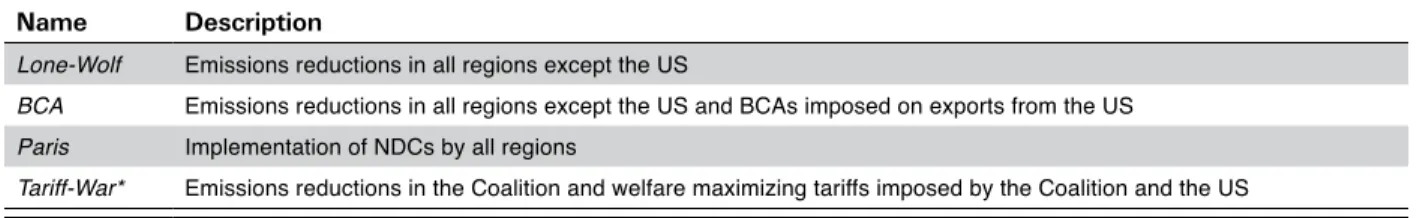
emissions are endogenous when it does not meet its Paris pledges, is determined endogenously in each scenario. Policy scenarios considered in the analysis are sum-marized in Table 3. In the first scenario, Lone-Wolf, all regions except the US reduce their CO2 emissions (and
there are no BCAs). In the second scenario, BCA, all re-gions except the US restrict emissions and tariffs, based on embodied CO2, are imposed on US exports of all
sec-tors except services. The third scenario, Paris, simulates emissions reductions pledged in NDCs under the Paris Climate Agreement in all regions (including the US). For computational reasons, our final policy scenario,
Tariff-War, is only implemented in the two-region,
sev-en-sector aggregation of the model described in Section 2.1. In this scenario, the US does not restrict emissions, the Coalition restricts emissions to meet the global Paris pledge, and the two regions impose welfare maximizing tariffs on each other’s exports of Other industry. This simulation is implemented by solving the model for, in one-percentage point increments, US and tariffs on Oth-er industry imports between 0% and 35%, Coalition tar-iffs on Other industry imports between 0% and 35%, and all combinations of those tariffs.
2.3 Border Carbon Adjustments & Embodied CO2 Emissions
In the BCA scenario, tariffs are used to retrospectively apply the carbon price in each importing region on emis-sions embodied in goods sourced from the US. The ad
valorem tariff imposed on imports of good i from the US
by region r ( ) is given by:
(1)
where is the price of a permit to release one ton of CO2 in region r, denotes tons of CO2 emissions
embodied in each unit of good i, and is the unit price of good i exported from the US.
Following Rutherford and Babiker (1997), our embod-ied emissions calculations include those from direct and indirect sources. Direct emissions are those that result from the combustion of fossil fuels in the sector in ques-tion, and indirect emissions are associated with interme-diate inputs. is calculated as:
(2)
where is direct emissions from the burning of fos-sil fuel f (coal, oil, gas) by industry i, is the quan-tity of intermediate input j used by industry i per unit of output, and is the share of intermediate input j sourced domestically, all in the US.We multiply by to prevent emissions embodied in imported inter-mediates from being charged twice—once when they are produced abroad and once when they are (incorporated in other goods) exported by the US. Applying equation (2) to each sector gives rise to a system of i equation and
i unknowns. We assign values for , and using the GTAP database and solve the system of equa-tion simultaneously to determine the value for each .
3. Results
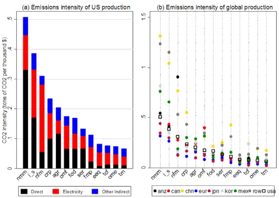
3.1 Sectoral Emissions Intensities & US Exports For each sector (except energy production sectors), Figure 2a illustrates the emissions intensity of produc-tion in the US and separately identifies direct emissions, emissions from electricity use, and emissions associated with other intermediate inputs. The four energy intensive sectors have the highest emissions intensities and elec-tricity is a large source of indirect emissions, especially for Non-metallic minerals. The emissions intensity of production across regions is compared in Figure 2b. In general, emissions intensities are highest in developing countries, especially China, and US emissions intensities are high relative to those in other developed countries. US exports by destination and sector (excluding energy production sectors) are reported in Figure 3. Excluding the Rest of the World, the EU (25.9%), Canada (11.7%), China (10.4%) and Mexico (8.6%) account for the largest share of US exports. The data also reveal that Non-metal-lic minerals (0.7%), Iron and steel (1.5%), and Non-fer-Table 3. Scenarios.
Name Description
Lone-Wolf Emissions reductions in all regions except the US
BCA Emissions reductions in all regions except the US and BCAs imposed on exports from the US
Paris Implementation of NDCs by all regions
Tariff-War* Emissions reductions in the Coalition and welfare maximizing tariffs imposed by the Coalition and the US * The Tariff-War scenario is only implemented in the two-region, seven-sector aggregation of the model.
rous metals (2.6%)—the three most emissions intensive goods—account for relative small proportions of total US exports. On the other hand, Chemical, rubber & plastic products, which is relatively emissions intensive, accounts for a significant share (14.8%) of US exports. 3.2 Paris Pledges & Border Carbon Adjustments Results from our modeling exercises are displayed in Table 4 (CO2 prices, welfare and US emissions) and
Figure 4 (US exports). In the Lone-Wolf scenario, CO2
prices, in 2011 dollars per metric ton (t) of CO2, are
high-est in Canada ($252/tCO2), the EU & EFTA ($181/tCO2),
Australia-New Zealand ($151/tCO2) and South Korea
($144/tCO2). Conversely, carbon prices are relatively low
in China ($5/tCO2) and Rest of World ($15/tCO2).
Proportional welfare changes reported in Table 4 are an-nual equivalent variation changes in consumer income relative to GDP (and do not account for benefits from avoided climate damages). Decreases in welfare are larg-est in Canada (3.1%), Australia–New Zealand (2.9%),
Figure 2. CO2 emissions intensity of production by sector.
Mexico (2.3%) and the EU & EFTA (2.2%). Despite a low carbon price, Rest of World also experiences a relatively large welfare decrease (1.5%) as it includes countries that are major crude oil exporters. Welfare decreases in Ja-pan (0.1%) and Korea (0.9%) are moderate as mitigation costs for these fossil fuel importers are partially offset by decreases in fossil fuel prices.
US welfare increases by 0.21% relative to BAU in the
Lone-Wolf scenario due to a fall in fossil fuel prices and
improved competitiveness in export markets. As illustrat-ed in Figure 4a, exports of Chemicals, rubber and plastic products experience the largest absolute increase in ex-ports, but the proportional change in these exports (2.6%) is less than that for Non-metallic minerals (9.4%), and Iron and steel (9.6%). The largest changes in exports involve US goods shipped to the EU. US emissions increase by 1.9%
relative to BAU due to decreased global fossil fuel prices and increased energy-intensive production, indicating leakage of emissions. Proportional emissions reductions in other regions are larger than those under each region’s Paris commitment, as these regions pursue deeper emis-sions reductions to hold global emisemis-sions constant. In the BCA scenario, the largest carbon tariff is 12.8% (Table 5) and applies to US Non-metallic minerals (the most CO2-intensive sector) exported to Canada (the
re-gion with the highest carbon price). Carbon tariffs on US energy-intensive goods exported to the EU range from 4.4% to 9.3%, and tariffs imposed by China and Rest of World are less than 1%. Carbon tariffs increase the CO2 prices in most regions as they increase the cost
of abating emissions by importing goods from the US. Despite the CO2 price increases, welfare in all non-US
re-Table 4. CO2 prices, welfare and emissions.
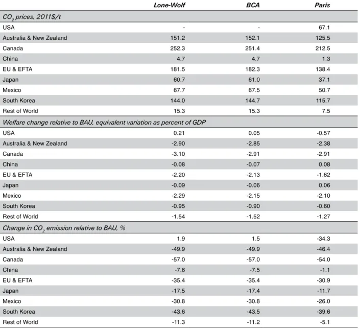
Lone-Wolf BCA Paris
CO2 prices, 2011$/t
USA - - 67.1
Australia & New Zealand 151.2 152.1 125.5
Canada 252.3 251.4 212.5 China 4.7 4.7 1.3 EU & EFTA 181.5 182.3 138.4 Japan 60.7 61.0 37.1 Mexico 67.7 67.5 50.7 South Korea 144.0 144.7 115.7 Rest of World 15.3 15.3 7.5
Welfare change relative to BAU, equivalent variation as percent of GDP
USA 0.21 0.05 -0.57
Australia & New Zealand -2.90 -2.85 -2.38
Canada -3.10 -2.91 -2.91 China -0.08 -0.07 0.08 EU & EFTA -2.20 -2.13 -1.62 Japan -0.09 -0.06 0.06 Mexico -2.29 -2.15 -2.10 South Korea -0.95 -0.90 -0.60 Rest of World -1.54 -1.52 -1.27
Change in CO2 emission relative to BAU, %
USA 1.9 1.5 -34.3
Australia & New Zealand -49.9 -49.9 -46.4
Canada -57.0 -57.0 -54.0 China -7.6 -7.5 -1.1 EU & EFTA -35.4 -35.4 -30.9 Japan -17.5 -17.4 -11.7 Mexico -30.8 -30.8 -26.0 South Korea -43.6 -43.5 -39.6 Rest of World -11.3 -11.2 -5.1
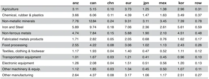
Figure 4. Absolute (right axis, bars) and proportion (left axis, dots) in the value of uS exports relative to BAu. Table 5. Ad valorem tariffs on uS exports in the BCA scenario, %.
anz can chn eur jpn mex kor row
Agriculture 3.11 5.15 0.10 3.73 1.25 1.38 2.96 0.31 Chemical, rubber & plastics 3.66 6.06 0.11 4.39 1.47 1.63 3.49 0.37 Non-metallic minerals 7.76 12.84 0.24 9.31 3.11 3.45 7.39 0.78 Iron and Steel 5.89 9.74 0.18 7.06 2.36 2.61 5.61 0.59 Non-ferrous metals 4.74 7.84 0.15 5.68 1.90 2.10 4.51 0.48 Fabricated metals products 1.71 2.82 0.05 2.05 0.68 0.76 1.62 0.17 Food processing 2.55 4.22 0.08 3.06 1.02 1.13 2.43 0.26 Textiles, clothing & footwear 1.17 1.93 0.04 1.40 0.47 0.52 1.11 0.12 Transportation equipment 1.01 1.67 0.03 1.21 0.41 0.45 0.96 0.10 Electronic equipment 1.26 2.08 0.04 1.51 0.51 0.56 1.20 0.13 Other machinery & equip. 1.12 1.85 0.03 1.34 0.45 0.50 1.07 0.11 Other manufacturing 2.64 4.37 0.08 3.17 1.06 1.17 2.51 0.27
gions increases relative to the Lone-Wolf scenario due to terms-of-trade improvements at the expense of the US. Welfare decreases in the US, but there is still a small wel-fare increase relative to BAU. US exports, relative to BAU, decrease for most commodities, and are proportionally the largest for Non-ferrous metals (12.5%), Non-metallic minerals (9.5%), and Chemical rubber & plastic prod-ucts (5.4%) (Figure 4b). These changes are driven by de-creased exports to Canada and the EU with exports to China and Rest of World, which impose relative low car-bon tariffs, increasing. US exports of services, which are not subject to a BCA, increase to all regions. The carbon tariffs result in a small reduction in US emissions and US emissions still increase to relative to BAU.
In the Paris scenario, a US carbon price of $67/tCO2 is
required to meet its NDC emissions reduction target. US exports for all commodities decrease with the larg-est proportional reductions occurring for the four en-ergy-intensive industries (Figure 4c). Welfare in the US falls by 0.57% relative to BAU. As US welfare in this sce-nario is significantly higher than in the BCA case, this indicates that BCAs would not be sufficient to make it economically advantageous for the US to implement pol-icies to meet its Paris pledges.
Due to emissions reductions in the US, carbon prices decrease elsewhere relative to the Lone-Wolf scenario, as less mitigation is required to meet the global constraint on CO2 emissions. Consequently, welfare is higher in
each non-US region in the Paris scenario than in the
Lone-Wolf scenario. Welfare increases due to the
con-straint on US emissions are smallest for the regions that trade intensively with the US (Canada and Mexico) as US exports become more expensive and the decrease in US income reduces demand for their exports.
3.3 A Tariff War
Welfare changes and CO2 prices from simulating our
sce-narios (including the Tariff-War case) when the model represents two regions and six sectors are displayed in Table 6. Estimated welfare changes in the US from the
more aggregated version of the model in the first three scenarios are qualitatively similar to those in Table 4: (1) The US experiences a small welfare gain when it does not restrict emissions and other nations do, (2) BCAs result in a small reduction in US welfare, and (3) meeting its Paris pledge results in a moderate reduction in US wel-fare. In the BCA scenario, the Coalition imposes a 0.28% tariff on Other industry goods produced in the US. The Nash equilibrium in the Tariff-War scenario occurs when the US imposes a tariff of 19% on Other industry imports and the Coalition imposes a 23% tariff on these goods. The tariff war results in a decrease in US welfare that is more than double that in the Paris scenario, indi-cating that when faced with the threat of a tariff war the best play for the US is to meet its Paris pledge (and avoid a tariff war). In the Coalition, welfare is higher when there are BCAs than in the Tariff-War scenario, indicat-ing that, in simple one-shot game, the Coalition also has an incentive to avoid a tariff war and the BCA scenario represents the Nash equilibrium.
Focusing on the simple one-shot Nash equilibrium, how-ever, ignores other important considerations. First, the Coalition may derive utility by enforcing ‘fairness’, and this utility gain not considered in our simulations may offset the welfare decrease simulated in the Tariff-War scenar-io relative to the BCA scenarscenar-io. Second, the experimental economics literature has shown that agents that coop-erate are willing to punish free-riding, even if it is costly for them (Fehr and Gächter, 2000). Additionally, the US, under the Trump administration, has indicated that it is willing to use trade measures to increase domestic welfare. If the US pursues such policies, the optimal strategy for the coalition is to impose a welfare maximizing tariff.
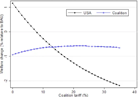
To illuminate possible outcomes, Figure 5 reports welfare changes in the two regions for alternative values of the Co-alition tariff when the US imposes a welfare maximizing tariff (conditional on the coalition tariff) and the Coali-tion reduces emission to meet the global Paris pledge. The optimal US tariff is 18% for values of the Coalition tariff Table 6. CO2 prices and welfare from the two-region, six sector model.
Lone-Wolf BCA Paris Tariff-War
CO2 prices, 2011$/t
USA - - $66.2
-Coalition $18.5 $18.5 $10.1 $18.7
Welfare change relative to BAU, equivalent variation as percent of GDP
USA 0.02 -0.02 -0.72 -1.50
Coalition -0.40 -0.39 -0.21 -0.57
Change in CO2 emission relative to BAU, %
USA 1.3 1.3 -34.3 -0.8
less than or equal to 18%, 19% for Coalition tariff values between 14% and 24%, 20% for Coalition tariffs between 25% and 34%, and 21% when the Coalition tariff is 35%. US welfare is a decreasing function of the tariff imposed by the Coalition and US welfare falls by 2.2% relative to BAU when the Coalition imposes a 35% tariff. The change in Coalition welfare is negative for all Coalition tariffs because this region reduces emissions and faces optimal US tariffs. At low tariffs, an increase in the Coalition tariff leads to relative large increases in welfare in this region. Coalition welfare is maximized when it imposes a 23% tariff and increases in the tariff beyond this value lead to relative small reductions in coalition welfare.
Figure 5 reveals two key outcomes. First, proportional US welfare losses from a tariff are much larger than those in the Coalition. Second, by imposing a tariff higher than the welfare maximizing one, the Coalition can inflict rel-atively large welfare decreases on the US while incurring small welfare decreases. A uniform response from the Coalition would, however, require a high level of coor-dination and possibly also income transfers among these regions. Nevertheless, our results indicate that there is scope for the Coalition to use tariffs as a mechanism to enforce the US to implement climate policies.
4. Conclusions
Avoiding undesirable human-induced climate change will require multilateral cooperation between nations. The Paris Agreement attempts to achieve this goal but meeting planned emissions reduction will rely on coun-ties voluntarily agreeing to stay in the accord. The ab-sence of legal channels to enforce this agreement means
that other measures will be required to persuade nations to achieve emission reduction targets. BCAs are one such mechanism and this paper quantitatively evaluated the impact of these tariffs using an economy-wide model with energy sector detail. As there are several indications that the current US Administration may withdraw the US from the Agreement or fail to meet its commitments, we considered a case where all countries except the US enact policies to reduce emissions and trade measures— BCAs and welfare-maximizing tariffs—are imposed on US exports.
In our analysis, BCAs imposed by each region were a function of the carbon price in that region and emissions embodied in US exports. The required carbon tariffs were quite low (less than 5%) in most cases, and higher tariffs (up to 13%) only applied to a small share of US exports and could be avoided by re-routing exports to regions with lower BCAs. Consequently, BCAs had only a small negative impact on US emissions and welfare. As US welfare was significantly lower when it met its Par-is pledge than when it faced BCAs but did not regulate GHG emissions, we conclude that BCAs will not be ef-fective in enforcing climate commitments.
In contrast, welfare changes were relatively large in the Nash equilibrium of tariff war between the US and the Co-alition (the rest of the world). US welfare under a tariff war was significantly lower than when it restricted emissions to meet its Paris pledge (and avoided the tariff war). While the final outcome will depend on the objective of the coalition and the behavior of the US, these results indicate that there is scope to use carefully chosen tariffs as an enforcement tool against regions that fail to meet their Paris pledges.
5. References
Aguiar, A., B. Narayanan & R. McDougall, 2016: An Overview of the GTAP 9 Data Base. Journal of Global Economic Analysis 1(1): 181–208.
Aldy, J. ,W. Pizer, M. Tavoni, L.A. Reis, K. Akimoto, G. Blanford, C. Carraro, L.E. Clarke, J. Edmonds, G.C. Iyer, H. C. McJeon, R. Richels, S. Rose & F. Sano, 2016: Economic tools to promote transparency and comparability in the Paris Agreement. Nature
Climate Change 6, 1000–1004.
Armington, P.S., 1969: A theory of demand for products distinguished by place of production. IMF Staff Papers, 16, 159–176.
Babiker, M.H. & T.F. Rutherford, 2005: The Economic Effects of Border Measures in Subglobal Climate Agreements. Energy
Journal 26(4): 99–125.
Baker, J.A. III, M. Feldstein, T. Halstead, N.G. Mankiw, H.M. Paulson, Jr., G.P. Shultz, T. Stephenson & R. Walton, 2017. The Conservative Case
for Carbon Dividends. Climate Leadership Council, Washington
DC. Retrieved from https://www/clcouncil.org/wpcontent/
uploads/2017/02/TheConservativeCaseforCarbonDividends.pdf.
Böhringer, C., E.J. Balistreri & T.F. Rutherford, 2012: The role of border carbon adjustment in unilateral climate policy: Overview of an Energy Modeling Forum study (EMF 29). Energy Economics 34(Suppl 2): S97–S110.
Burniaux, J-M, J. Château & R. Duval, 2010: Is there a case for carbon-based border tax adjustments? An applied general equilibrium analysis. Economics Department Working Paper No.
794, OECD.
Chen, Y.-H., S. Paltsev, J.M. Reilly, JF. Morris & M.H. Babiker, 2016: Long-term economic modeling for climate change assessment.
Economic Modeling 52(B): 867–883.
Demailly, D. & P. Quirion, 2008. European Emissions Trading Scheme and Competitiveness: A Case study on the Iron and Steel Industry. Energy Economics 30(4): 2009–27.
DiChrstopher, T., 2017: EPA chief Scott Pruitt says carbon dioxide is not a primary contributor to global warming. CNBC, 3/9/2017. Retrieved from http://www.cnbc.com.
Dirkse, S.P. & M.C. Ferris, 1995: The PATH Solver: a non-monontone stabilization scheme for Mixed Complementarity Problems.
Optimization Methods and Software 5: 123–156.
Doyle, A. & R. Rampton, 2016: Paris climate accord to take effect; Obama hails ‘historic day’. Reuters, 10/5/2016. Retrieved from
http://www.reuters.com.
Felder, S. & T.F. Rutherford, 1993: “Unilateral CO2 Reduction and Carbon Leakage.” Journal of Environmental Economics and
Management 25(2): 163–176.
Fehr, E. & S. Gächter, 2000: Cooperation and punishment in public goods experiments. The American Economic Review 90(4): 980–996.
Gillespie, P., 2017: Trump slaps first tariffs on Canadian lumber.
The Cable News Network, 4/25/2017. Retrieved from http:// www.cnn.com.
Hertel, T., D. Hummels, M. Ivanic & R. Keeney, 2007: How Confident can we be of CGE-Based Assessments of Free Trade Agreements?
Economic Modelling 24(4): 611–635.
Jacoby, H., Y.-H., Chen & B. Flannery, 2017: Transparency in the Paris
Agreement. Joint Program on the Science and Policy of Global
Change Report 308, Massachusetts Institute of Technology. Kemp, L. 2016: US-proofing the Paris Climate Agreement, Climate
Policy, 17(1): 86–101.
Lanz, B. & T. Rutherford, 2016: GTAPinGAMS: Multiregional and small open economy models. Journal of Global Economic Analysis, 1(2): 1–77.
Liptak, K. & D. Merica, 2017: Trump agrees ‘not to terminate NAFTA at this time’. The Cable News Network, 4/27/2017. Retrieved from
http://www.cnn.com.
Mathiesen, K., 2016: January 20, 2018: The day US could leave the Paris Agreement. Climate Home, 9/11/2016. Retrieved from
http://www.climatechangenews.com/.
Merica, D., 2017: Trump dramatically changes US approach to climate change. The Cable News Network, 3/29/2017. Retrieved from
http://www.cnn.com.
Mattoo, A., A. Subramanian, D. van der Mensbrugghe & J. He, 2009: Reconciling Climate Change and Policy. World Bank Policy Research Working Paper no. WPS 5123.
OECD, 2014: Long-term baseline projections, No. 95 (Edition 2014), OECD Economic Outlook: Statistics and Projections (database). DOI: 10.1787/data-00690-en (Accessed 4/24/2017)
Paltsev, S., J. Reilly, H.D. Jacoby, R.S. Eckaus, J. McFarland,
M. Sarofim, M. Asadooria & M. Babiker, 2005. The MIT Emissions
Prediction and Policy Analysis (EPPA) Model: Version 4. Joint
Program on the Science and Policy of Global Change Report 125, Massachusetts Institute of Technology.
Peters, J., 2016: The GTAP-Power Data Base: Disaggregating the electricity sector in the GTAP Data Base. Journal of Global
Economic Analysis 1(1): 209–250.
Ponssard, J-P. & N. Walker, 2008: EU emissions trading and the cement sector: A spatial competition analysis. Climate Policy 8(5): 467–93.
Rosenthal, E.R., 2012: GAMS - A User’s Guide. GAMS Development Corporation, Washington DC.
Rutherford, T.F. & M. Babiker, 1997: Input-Output and general equilibrium estimates of embodied carbon: A dataset and static framework for assessment. Economics Discussion Paper 97–02, University of Colorado, Boulder.
Rutherford, T.F. & S. Paltsev, 2000: GTAP-Energy in GAMS: The Dataset and Static Model. Economics Discussion Paper 00–02, University of Colorado, Boulder.
Rutherford, T.F., 1995: Extension of GAMS for complementary problems arising in applied economic analysis. Journal of
Economics Dynamics and Control 19(8): 1299–1324.
Sakari, M. & J. Barrett, 2016: Border carbon adjustments: Addressing emissions embodied in trade, Energy Policy 92: 102–110. Stutter, J.D., 2017: The Paris Agreement is bigger than Trump ... isn’t
it? The Cable News Network, 2/22/2017. Retrieved from http://
www.cnn.com.
Vandyck, T., K. Keramidas, B. Saveyn, A. Kitous & Z. Vrontisi, 2016: A global stocktake of the Paris pledges: Implications for energy systems and economy. Global Environmental Change 41: 46–63. US Congress, 2009: The American Clean Energy and Security Act of
2009 (H.R. 2454). US House of Representatives, Washington, DC.
Winchester, N., 2012: The impact of border carbon adjustments under alternative producer responses. American Journal of Agricultural
Economics 94(2): 354–359.
Winchester, N., S. Paltsev & J.M. Reilly, 2011: Will border carbon adjustments work? The B.E. Journal of Economic Analysis & Policy 11(1), Article 7.
Wong, E., 2016: Trump has called climate change a Chinese hoax. Beijing says it is anything but. New York Times, 11/18/2016. Retrieved from http://www.nytimes.com.
For limited quantities, Joint Program Reports are available free of charge. Contact the Joint Program Office to order. Complete list: http://globalchange.mit.edu/publications
MIT Joint Program on the Science and Policy
of Global Change Massachusetts Institute of Technology 77 Massachusetts Ave., E19-411 Cambridge MA 02139-4307 (USA)
T (617) 253-7492 F (617) 253-9845 [email protected]
http://globalchange.mit.edu/ 312. Can Tariffs be Used to Enforce Paris Climate Commitments?
Winchester, June 2017
311. A Review of and Perspectives on Global Change Modeling for Northern Eurasia. Monier et al., May 2017
310. The Future of Coal in China. Zhang et al., Apr 2017
309. Climate Stabilization at 2°C and Net Zero Carbon Emissions.
Sokolov et al., Mar 2017
308. Transparency in the Paris Agreement. Jacoby et al., Feb 2017
307. Economic Projection with Non-homothetic Preferences: The Performance and Application of a CDE Demand System.
Chen, Dec 2016
306. A Drought Indicator based on Ecosystem Responses to Water Availability: The Normalized Ecosystem Drought Index. Chang et al., Nov 2016
305. Is Current Irrigation Sustainable in the United States? An Integrated Assessment of Climate Change Impact on Water Resources and Irrigated Crop Yields. Blanc et al., Nov 2016
304. The Impact of Oil Prices on Bioenergy, Emissions and Land Use. Winchester & Ledvina, Oct 2016
303. Scaling Compliance with Coverage? Firm-level Performance in China’s Industrial Energy Conservation Program. Karplus et al., Oct 2016
302. 21st Century Changes in U.S. Heavy Precipitation Frequency
Based on Resolved Atmospheric Patterns. Gao et al., Oct 2016
301. Combining Price and Quantity Controls under Partitioned Environmental Regulation. Abrell & Rausch, Jul 2016
300. The Impact of Water Scarcity on Food, Bioenergy and Deforestation. Winchester et al., Jul 2016
299. The Impact of Coordinated Policies on Air Pollution Emissions from Road Transportation in China. Kishimoto et al., Jun 2016
298. Modeling Regional Carbon Dioxide Flux over California using the WRF-ACASA Coupled Model. Xu et al., Jun 2016
297. Electricity Investments under Technology Cost Uncertainty and Stochastic Technological Learning. Morris et al., May 2016
296. Statistical Emulators of Maize, Rice, Soybean and Wheat Yields from Global Gridded Crop Models. Blanc, May 2016
295. Are Land-use Emissions Scalable with Increasing Corn Ethanol Mandates in the United States? Ejaz et al., Apr 2016
294. The Future of Natural Gas in China: Effects of Pricing Reform and Climate Policy. Zhang & Paltsev, Mar 2016
293. Uncertainty in Future Agro-Climate Projections in the United States and Benefits of Greenhouse Gas Mitigation.
Monier et al., Mar 2016
292. Costs of Climate Mitigation Policies. Chen et al., Mar 2016
291. Scenarios of Global Change: Integrated Assessment of Climate Impacts. Paltsev et al., Feb 2016
290. Modeling Uncertainty in Climate Change: A Multi-Model Comparison. Gillingham et al., Dec 2015
289. The Impact of Climate Policy on Carbon Capture and Storage Deployment in China. Zhang et al., Dec 2015
288. The Influence of Gas-to-Liquids and Natural Gas Production Technology Penetration on the Crude Oil-Natural Gas Price Relationship. Ramberg et al., Dec 2015
287. Impact of Canopy Representations on Regional Modeling of Evapotranspiration using the WRF-ACASA Coupled Model.
Xu et al., Dec 2015
286. Launching a New Climate Regime. Jacoby & Chen, Nov 2015
285. US Major Crops’ Uncertain Climate Change Risks and Greenhouse Gas Mitigation Benefits. Sue Wing et al., Oct 2015
284. Capturing Natural Resource Dynamics in Top-Down Energy-Economic Equilibrium Models. Zhang et al., Oct 2015
283. Global population growth, technology, and Malthusian constraints: A quantitative growth theoretic perspective.
Lanz et al., Oct 2015
282. Natural Gas Pricing Reform in China: Getting Closer to a Market System? Paltsev & Zhang, Jul 2015
281. Impacts of CO2 Mandates for New Cars in the European
Union. Paltsev et al., May 2015
280. Water Body Temperature Model for Assessing Climate Change Impacts on Thermal Cooling. Strzepek et al., May 2015
279. Emulating maize yields from global gridded crop models using statistical estimates. Blanc & Sultan, Mar 2015
278. The MIT EPPA6 Model: Economic Growth, Energy Use, and Food Consumption. Chen et al., Mar 2015
277. Renewables Intermittency: Operational Limits and Implications for Long-Term Energy System Models. Delarue & Morris, Mar 2015
276. Specifying Parameters in Computable General Equilibrium Models using Optimal Fingerprint Detection Methods.