Numerical Modeling and High Speed Parallel Computing: New Perspectives for Tomographic Microwave Imaging for Brain Stroke Detection and Monitoring

HAL Id: hal-01356092

https://hal.archives-ouvertes.fr/hal-01356092

Preprint submitted on 24 Aug 2016

HAL is a multi-disciplinary open access

archive for the deposit and dissemination of

sci-entific research documents, whether they are

pub-lished or not. The documents may come from

teaching and research institutions in France or

abroad, or from public or private research centers.

L’archive ouverte pluridisciplinaire HAL, est

destinée au dépôt et à la diffusion de documents

scientifiques de niveau recherche, publiés ou non,

émanant des établissements d’enseignement et de

recherche français ou étrangers, des laboratoires

publics ou privés.

Distributed under a Creative Commons Attribution| 4.0 International License

Computing: New Perspectives for Tomographic

Microwave Imaging for Brain Stroke Detection and

Monitoring

Pierre-Henri Tournier, Marcella Bonazzoli, Victorita Dolean, Francesca

Rapetti, Frédéric Hecht, Frédéric Nataf, Iannis Aliferis, Ibtissam El Kanfoud,

Claire Migliaccio, Maya de Buhan, et al.

To cite this version:

Pierre-Henri Tournier, Marcella Bonazzoli, Victorita Dolean, Francesca Rapetti, Frédéric Hecht, et

al.. Numerical Modeling and High Speed Parallel Computing: New Perspectives for Tomographic

Microwave Imaging for Brain Stroke Detection and Monitoring. 2016. �hal-01356092�

For Review Only

Abstract—This paper deals with microwave tomography for

brain stroke imaging using state-of-the-art numerical modeling and massively parallel computing. Microwave tomographic imaging requires the solution of an inverse problem based on a minimization algorithm (e.g. gradient based) with successive solutions of a direct problem such as the accurate modeling of a whole-microwave measurement system. Moreover, a sufficiently high number of unknowns is required to accurately represent the solution. As the system will be used for detecting the brain stroke (ischemic or hemorrhagic) as well as for monitoring during the treatment, running times for the reconstructions should be reasonable. The method used is based on high-order finite

elements, parallel preconditioners from the Domain

Decomposition method and Domain Specific Language with open source FreeFEM++ solver.

Index Terms— High Performance Computing, Parallel

computers, Finite element analysis, Microwave antenna arrays, Electromagnetic Diffraction, Microwave Imaging, Biomedical Imaging, Inverse Problems

I. INTRODUCTION

Stroke, or cerebrovascular accident (CVA), is classically characterized as a neurological deficit attributed to an acute focal injury of the central nervous system (CNS) by a vascular cause, including cerebral infarction, intracerebral hemorrhage (ICH), and subarachnoid hemorrhage (SAH), and is a major cause of disability and death worldwide [1]. About 85% of strokes are ischemic due to cerebral infarction, caused by an interruption of the blood supply to some part of the brain, 15% are hemorrhagic (10% primary and 5% subarachnoid

F. Hecht, F. Nataf, and P.-H. Tournier are with LJLL, UPMC, CNRS, France and INRIA-Paris, EPC Alpines, France.

I. Aliferis, I. El Kanfoud, C. Migliaccio, Ch. Pichot are with Université Côte d'Azur, CNRS, LEAT, France.

M. Bonazzoli, V. Dolean, and F. Rapetti are with are with Université Côte d'Azur, CNRS, LJAD, France. V. Dolean is also with Université Côte d'Azur, CNRS, LEAT, France and Dept. Maths and Stats, U. Strathclyde, Glasgow, UK.

M. Darbas is with Université Picardie, Amiens, France.

M. de Buhan is with MAP5, Université Paris Descartes, Paris, France. S. Semenov, is with EMTensor GmbH, Vienna, Austria.

This work is supported by ANR grant MEDIMAX (ANR-13-MONU-0012).

hemorrhage) [2]. Differentiating between these different types of strokes is an essential part of the initial workup of the patients because the subsequent management and treatment of each patient is vastly different. Rapid and accurate diagnosis is crucial since the only drug currently approved by the FDA for treatment of acute ischemic stroke is intravenous tissue plasminogen activator (tPA) administered within 3 hours of stroke onset. Neuroimaging has to play a vital role in the workup of acute stroke by providing information essential to accurately triage patients, and expedite clinical decision-making with regards to treatment. CT and MRI [3] are actually the "gold" standards but they are bulky diagnostic instruments and cannot be used in continuous brain monitoring. A non-invasive and transportable/portable device would have clear clinical applications at the bedside in a Neurological Intensive Care Unit (NICU).

Microwave tomography is a novel, early development stage imaging modality with a large number of potential attractive medical applications. A difference between the dielectric properties (complex permittivity) of normal and diseased brain tissues is a great potential for this imaging modality. Detecting and identifying strokes is challenging as it corresponds to a small opposite variation of the permittivity values of brain tissues of about +/- 10 % of the baseline tissue values for the two types of strokes (ischemic or hemorrhagic) [4]. The rapid data acquisition time is another attractive feature of microwave tomography but rapid tomographic reconstructions are mandatory for developing a novel imaging modality with a new paradigm: detecting, identifying and monitoring stroke continuously during treatments by exposing head tissues to low-level microwave incident field and capturing the scattered signal by an array of antennas. Tomographic imaging requires the solution of an inverse problem based on a minimization algorithm. Reconstruction algorithms are computationally intensive with successive solutions of the forward problem needing efficient numerical modeling and high-performance parallel computing. A majority of works in the literature has made use of geometrically simple phantoms or with only a limited amount of tissue-mimicking materials. The modeling must have to accurately take account of the high heterogeneity and complexity of head tissues (skin, fat, skull, bone marrow,

Numerical Modeling and High Speed Parallel

Computing: New Perspectives for Tomographic

Microwave Imaging for Brain Stroke Detection and

Monitoring

Pierre-Henri Tournier, Marcella Bonazzoli, Victorita Dolean, Francesca Rapetti, Frédéric Hecht,

Frédéric Nataf, Iannis Aliferis, Ibtissam El Kanfoud, Claire Migliaccio, Maya de Buhan, Marion

For Review Only

brain/white matter, brain/grey matter, cerebrospinal fluid,

arteries, etc.) for normal cases and for different possible brain pathology cases (ischemic and hemorrhagic strokes, brain injuries, etc.). Another major point refers to the accurate modeling of the incident field from transmitting and receiving antennas. This interaction is very complex, as it must be seen as a coupling problem between the antennas and the head rather than a simple scattering problem. In addition, the electric field is measured by means of receiving antennas (sensors). Therefore, we do not have access directly to the electric field but only via antenna S parameters. The purpose of this work is to solve the inverse problem associated to a prototype developed by EMTensor GmbH (Vienna, Austria) [5] using state-of-the-art modeling, high-performance and massively parallel computing.

II. TOMOGRAPHICSYSTEM

The model of microwave imaging is based on BRain IMaging Generation1 (BRIMG1), a tomographic microwave system developed by EMTensor GmbH [5]. The system consists of a cylindrical metallic chamber composed of 5 rings of 32 Transmitting/Receiving antennas (Fig. 1). The antennas are ceramic (εr = 59) loaded open-ended waveguides. The diameter of the chamber is 285 mm with a height of 280 mm. The rings are 30 mm equally spaced, the first one being located at 40 mm from the top of the chamber. The chamber is filled with a matching liquid medium during measurements. The operating frequency of the system is 0.9 GHz to 1.8 GHz. The data acquisition cycle of the system is fully electronically controlled, allowing for a total data acquisition of about 30 s. The imaging chamber is in horizontal position, allowing easy positioning a human head within an imaging domain (Fig. 2). The head of the patient is introduced in the chamber as shown in Fig. 2. A special thin membrane is used for isolating the human head from the matching liquid and keeping the liquid within the chamber. A carbon loaded silicon rubber (CLSR) is also used for reducing reflection from boundary conditions (Fig. 3).

Fig. 1. Left: General view of BRIMG1(courtesy of EMTensor GmbH). Right: Computational domain.

A switching matrix connected to a network analyzer selects the transmitting and receiving antennas. The system is potentially delivering a 160 × 160 matrix of S parameters. The measured S parameters due to the scattered field of an object

under investigation are obtained by complex subtraction betweentwo measurements with empty chamber and with the head, respectively. The raw data can be wirelessly transferred to a remote computing center.

Fig. 2. BRIMG1: Human head measurement (courtesy of EMTensor GmbH)

Fig. 3. BRIMG1: Side sketch (courtesy of EMTensor GmbH). The HPC machine will compute the tomographic images, which can be quickly transferred from the computing center to the hospital.

III. FORWARDMODELING

We consider the domain Ω ⊂ R3 for representing the whole-chamber (Fig. 1) as an inhomogeneous dissipative nonmagnetic medium of complex permittivity

ε

(x)

. For each transmitting antenna j = 1, . . . N at radial frequency ω, the wave equation for the electric field vector

E

_j

(x)

with an

e

iωt

time-dependence is

∇ × (∇ × E

_j

) − k

2

E

_j

= 0 in Ω

(1) with

k

2

= k

2

(x) =

ω

2

ε

_r

(x)

ε

₀

µ

₀, where k(x) is the complex wavenumber of the inhomogeneous medium, ε0 and μ0 the permittivity and permeability of free space, respectively. The boundary conditions on the perfectly conducting parts Γc of the walls of the chamber are

For Review Only

where n is the unit outward normal to ∂Ω.

The impedance boundary conditions on the aperture of transmitting open-ended waveguide j and receiving waveguide i = 1,..., N, j ≠ i are

(∇ × E

_j

) × n + iβn × (E

_j

× n) = g

_j

on Γ

_j (2)

(∇ × E

_j

) × n + iβn × (E

_j

× n) = 0 on Γ

_i

, i ≠ j

(3) where β is the propagation constant of the TE10 fundamental mode of the waveguide. In equation (2) we impose an incident wave corresponding to the excitation of the fundamental mode

E

0_j

of the j-th waveguide with

g

_j

= (∇ × E

0_j

) × n + i

β

n × (E

_j0

× n)

(4) On the other hand, equation (3) corresponds to a first order Silver–Müller absorbing boundary condition, approximating a transparent boundary condition on the aperture of the receiving waveguide antenna i = 1,..., N, i ≠ j. On the bottom of the chamber we impose a metallic boundary condition, whereas we impose an impedance boundary condition on the top of the chamber. As a result, the whole boundary value problem for each transmitting antenna t = 1, . . . , N is to find

E

_j such that

∇ × (∇ × E

_j

) − k

2

E

_j

= 0 in Ω

E

_j

× n = 0 on Γ

c

(∇ × E

_j

) × n + i

β

n × (E

_j

× n) = g

_j

on Γ

_j

(∇ × E

j

) × n + i

β

n × (E

j

× n) = 0 on Γ

i

, i ≠ j

⎧

⎨

⎪

⎪

⎪

⎩

⎪

⎪

⎪

(5)

Now, let

V = v ∈ H(curl,Ω),v × n = 0 on Γ

{

_c

}

, where

H (curl,Ω) = v ∈ L

₂

(Ω)

3

_{,∇ × v ∈ L}

2

(Ω)

3

{

}

is the space of square integrable functions whose curl is also square integrable. For each transmitting antenna j = 1,..., N, the variational form of problem (5) is : find

E

_j

∈ V

such that

∇ × E

j

(

)

. ∇ × v

₍

₎

− k

2

E

j

.v

⎡

⎣

⎤

⎦

Ω

∫

+

_Γ

iβ E

(

j

× n

)

i 1=1 N

∪

∫

. v × n

₍

₎

=

_Γ

g

j j

∫

.v ∀v ∈V

(6) IV. HIGH-ORDER EDGE FINITE ELEMENTS

For using a finite element discretization of the variational problem, we introduce a tetrahedral mesh Th of the domain Ω and a finite dimensional subspace

V

_h

⊂ H (curl,Ω)

. A simple conformal discretization for space

H (curl,Ω)

is given by low order Nédélec edge finite elements of polynomial degree r = 1 [7].

In order to have a higher numerical accuracy with the same total number of unknowns, we consider a high order edge

element discretization, choosing the high order extension of Nédélec elements presented in [8] and [9].

We implemented edge elements of degrees 2 and 3 in FreeFem++, an open source domain specific language (DSL) specialized for solving boundary value problems by using variational discretizations (finite elements, discontinuous Galerkin, hybrid methods,...) [6]. High order elements can be used by loading the plugin Element Mixte3d and declaring the finite element space fespace using the keywords Edge13d,

Edge23d, respectively (standard edge elements of degree 1 are

already present in FreeFem++ and called Edge03d)

.

V. DOMAIN DECOMPOSITION PRECONDITIONING

The discretization of the problem presented in Section III using the high order edge finite elements described in Section IVproduces a linear system

Au

_j

= b

_j (7)

for each transmitting antenna j. Direct solvers are not suited for such large linear systems arising from complex three dimensional models because of their high memory cost. On the other hand, matrices resulting from high order discretizations are ill conditioned as shown numerically in [8] for similar problems, and preconditioning becomes necessary when using iterative solvers.

Domain decomposition preconditioners are naturally suited to parallel computing and make it possible to deal with smaller subproblems [13]. The domain decomposition preconditioner we employ is called Optimized Restricted Additive Schwarz (ORAS)

M

_ORAS−1

=

R

s T

_D

s

A

s −1

_R

s s=1 N_sub

∑

(8)

where Nsub is the number of overlapping subdomains Ωs into which the domain Ω is decomposed (Fig. 4). Here, the matrices As are the local matrices of the subproblems with impedance boundary conditions (∇ × E) × n + i

ϖ

n × (E × n) as transmission conditions at the interfaces between subdomains. This preconditioner is an extension of the restricted additive Schwarz method proposed by Cai and Sarkis [15], but with more efficient transmission conditions between subdomains than Dirichlet conditions [16].

In order to describe the matrices Rs, Ds, let N be an ordered set of the unknowns of the whole domain and let

N =

N

_s

s=1 Nsub

∪

be its decomposition into the (non disjoint) ordered subsets corresponding to the different (overlapping) subdomains Ωs. The matrix Rs is the restriction matrix from Ω to the subdomain Ωs: it is a #Ns × #N Boolean matrix and its (i, j) entry is equal to 1 if the i-th unknown in Ns is the j-th one in N. Notice that

R

_sT is then the extension matrix from the subdomain Ωs to Ω. The matrix Ds is a #Ns × #Ns diagonal matrix that gives a discrete partition of unity, i.e.

For Review Only

R

_sT

_D

s

R

s

s=1

Nsub

∑

= I

; in particular the matrices D deal with the unknowns that belong to the overlap between subdomains.The preconditioner without the partition of unity matrices Ds,

M

_ORAS−1

=

R

_sT

D

_s

A

_s−1

R

_s

s=1 N_sub

∑

which is called Optimized Additive Schwarz (OAS), would be symmetric for symmetric problems, but in practice it gives a slower convergence with respect to

M

_ORAS−1 [10].These domain decomposition preconditioners are implemented in the HPDDM library [12], an open source high-performance unified framework for domain decomposition methods. HPDDM can be interfaced with various programming languages and open source finite element libraries such as FreeFem++, which we use in the simulations.

Fig. 4. Computational domain divided into 128 subdomains.

VI. NUMERICAL RESULTS

A. Comparison with Experimental Measurements

The measured physical quantities are the S parameters of the scattering matrix, which are the complex reflection and

transmission coefficients measured by the 160 receiving

antennas when a signal is transmitted by one of the 160 transmitting antennas. A set of measurements then consists in a complex matrix of size 160 × 160. In order to compute the numerical counterparts of these reflection and transmission coefficients, we use the following formula, which is appropriate in the case of open-ended waveguides

S

_ij

=

E

_j

.E

_i0 Γi

∫

E

_i02 Γi

∫

, i ≠ j

(9)

where Ej is the solution of the problem (5) when the j-th waveguide antenna transmits the signal, and

E

_i0

is the TE10 fundamental mode of the i-th receiving waveguide (

E

_j denotes the complex conjugate of

E

_j). The

S

_ijwith i ≠ j

denote the transmission coefficients, and

S

_ii the reflection coefficients.

For a comparison of the computed coefficients

S

_ijwith the measured ones, the imaging chamber is filled with a homogenous matching solution in order to reduce the return loss of the ceramic-loaded waveguide antennas and to match with the average brain tissues. The relative complex permittivity of the matching solution chosen for the experiments and numerical solution at frequency f = 1 GHz is

ε

matching= 44 − i20. The relative permittivity inside the ceramic-loaded waveguides is

_ε

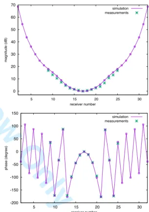
ceramics= 59, assuming a lossless ceramic material.

Fig. 5. Normalized amplitude (top) and phase (bottom) between the computed and measured S-parameters.

For this test case, the set of experimental data consists in S parameters from the 160 receiving antennas when each antenna from the second ring from the top is transmitting. Figure 4 shows the normalized magnitude (dB) and phase (degree) of the complex coefficients

S

_ijcorresponding to a transmitting antenna in the second ring from the top and to the 31 receiving antennas in the middle ring (note that measured coefficients are available only for 17 receiving antennas). The computed coefficients are obtained by solving the direct problem with edge finite elements of polynomial degree r = 2. The normalization is done by dividing every transmission

0 10 20 30 40 50 60 70 5 10 15 20 25 30 magnitude (dB) receiver number simulation measurements -200 -150 -100 -50 0 50 100 150 5 10 15 20 25 30 phase (degree) receiver number simulation measurements

For Review Only

coefficient by the transmission coefficient corresponding to

the receiving antenna directly opposite to the transmitting antenna, which is thus set to 1. Since we normalize with respect to the coefficient having the lowest expected magnitude, the magnitude of the transmission coefficients shown in Fig. 5 is larger than 0 dB. We can see that the transmission coefficients computed from the simulation are in very good agreement with the measurements.

B. High-Order Element Efficiency

The goal of the following numerical experiments is to assess the efficiency of the high order finite elements described in Section IV compared to the classical lowest order edge elements in terms of accuracy and computing time, which are of great importance for such an application for brain imaging. For this test case, a non dissipative plastic-filled cylinder of diameter 6 cm and relative permittivity

ε

cyl= 3 is inserted in the imaging chamber with same background matching medium as defined in Section A. We consider the 32 antennas of the second ring as transmitting antennas at frequency f = 1 GHz, and all the 160 antennas are receiving.

Fig. 6. Cross-Section of the chamber showing the magnitude of the real part of the total field E in the chamber with the plastic tube.

We evaluate the error on the reflection and transmission coefficients Sij with respect to the coefficients

S

_ijref computed from a reference solution. The error is calculated with the following formula err = S_ij− S_ijref 2 j,i

∑

S_ijref 2 j,i

∑

(10)

The reference solution is computed on a fine mesh of approximately 18 million tetrahedra using edge finite elements of degree r = 2, resulting in 114 million unknowns. The section in Fig. 6 shows the computational domain and the magnitude of the real part of the total field E over the

cross-section when one antenna of the second ring from the top is transmitting. We compare the computing time and the relative error (10) for different numbers of unknowns corresponding to several mesh sizes, for approximation degrees r = 1 (15 pts/λ) and 2 (10 pts/λ) (Table I). We report the results on Fig. 7 and 8. All these simulations are carried out using 512 subdomains with one MPI process and two OpenMP threads per subdomain, for a total of 1024 cores on the Curie supercomputer ( http://www-hpc.cea.fr/fr/complexe/tgcc-curie.htm).

Degree 1 Time

(s) Error Degree 2 Time (s) Error

# unknowns # unknowns 2,373,214 22 0.384 1,508,916 39 0.242 8,513,191 53 0.184 5,181,678 62 0.099 21,146,710 130 0.117 12,693,924 122 0.057 42,538,268 268 0.083 26,896,130 236 0.036 73,889,953 519 0.068 45,781,986 396 0.019 Table I. Total number of unknowns, computing time (seconds), and relative error on computed Sij.

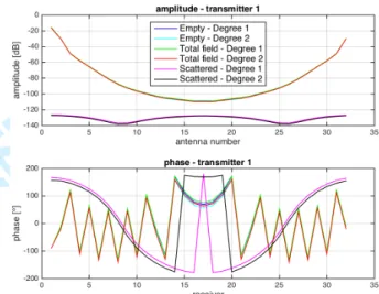
Fig. 7. Comparison between degrees r=1 and r=2 on empty, total and scattered fields (amplitude and phase).

Fig. 8. Computation time (seconds) and relative error on computed Sij using elements of degree r=1 and r=2 for different mesh sizes and number of unknowns in millions.

0.01 0.1 1 0 50 100 150 200 250 300 350 400 450 500 550 2.4M 8.5M 21M 43M 74M 1.5M 5.2M 13M 27M 46M relative error time to solution (s) Degree 1 Degree 2

For Review Only

As we can see, the higher order approximation (r = 2) allows a

given accuracy with much fewer unknowns and much less computation time than the lowest order approximation (r=1). For example, at a given accuracy err of E ≈ 0.1, the finite element discretization of degree r=1 requires 21 million unknowns and a computing time of 130 seconds, while the high order finite element discretization (r=2) only needs 5 million unknowns, with a corresponding computing time of 62 seconds. It turns out we obtain the same accuracy with 10 points per wavelength with degree r=2 than with 20 points per wavelength with degree r =1.

VII. INVERSE PROBLEM

A. Mathematical Formulation

The inverse problem that we consider consists in finding the unknown complex dielectric permittivity

ε

(x)

in Ω, such that the solutions

E

_j

(x)

, j = 1,...,N of problem (4) lead to corresponding scattering parameters S (14) that coincide with the measured scattering parameters

S

_ijmeas, for i, j = 1, . . . , N. Let

κ = k

2 be the unknown complex parameter of the inverse problem, and let us denote by

E

_j

(

κ

)

the solution of the direct problem (5) with the complex dielectric permittivity ε. The corresponding scattering parameters will be denoted by

S

_ij

(κ )

for i, j = 1, . . . , N.

The misfit of the parameter

κ

to the data can be defined with the following cost functional

J (κ) =

1

2

S

ij

(κ) − S

ij meas2 i=1 N

∑

j=1 N

∑

=

1

2

E

_j

(κ).E

i 0 Γi

∫

E

_i02 Γi

∫

− S

_ijmeas 2 i=1 N

∑

j=1 N

∑

(11)

In a classical way, solving the inverse problem consists in minimizing the functional J with respect to the parameter

κ

. Computing the differential of J in a given arbitrary direction

δκ

yields DJ (κ,δκ) = Re (S_ij(κ) − Sij meas₎ δ Ej(κ).Ei 0 Γi

∫

E_i02 Γi

∫

⎡ ⎣ ⎢ ⎢ ⎢ ⎤ ⎦ ⎥ ⎥ ⎥ i=1 N

∑

j=1 N

∑

(12)

for

δκ ∈ C

and where

δ

E

_j

(

κ

)

is the solution of the following linearized problem

∇ × ∇ ×δ E

(

j

)

−κδ Ej=δκ Ej in Ω δ Ej× n = 0 on Γc ∇ ×δ Ej

(

)

× n + iβn × δ E

(

j× n

)

= 0 on Γi,i =1,..., N ⎧ ⎨ ⎪ ⎪ ⎩ ⎪ ⎪ (13)

We now use the adjoint approach in order to simplify the expression of DJ. This will allow us to compute the gradient efficiently after discretization, with a number of computations independent of the size of the parameter space.

Introducing the solution

F

_j

(

κ

)

of the following adjoint problem

∇ × ∇ × F

(

j

)

−

κ F

j

= 0 in Ω

F

_j

× n = 0 on Γ

c

∇ × F

_j

(

)

× n + iβn × F

(

_j

× n

)

=

S

_ij

(κ ) − S

ij meas

(

)

E

_i02 Γi

∫

E

_i0

_{on Γ}

i

,i =1,..., N

(14)

we get after some integration by parts (not detailed here) δκ Ej.Fj Ω

∫

= (S_ij(κ) − Sij meas₎ Ei 0_.δE j Γi

∫

E_i02 Γi

∫

⎡ ⎣ ⎢ ⎢ ⎢ ⎤ ⎦ ⎥ ⎥ ⎥ i=1 N

∑

(15) Finally, the differential of J can be computed as

DJ (

κ

,

δκ

) =

Re

_⎣

⎡

∫

_Ω

δκ

E

j

.F

j

⎤

_⎦

j=1 N

∑

(16) We can then compute the gradient to use in a gradient-based local optimization algorithm. The numerical results presented in Section B are obtained using a limited-memory Broyden-Fletcher-Goldfarb-Shanno (L-BFGS) algorithm. Note that every evaluation of J requires the solution of the state problem (5) while the computation of the gradient requires the solution of (5) as well as the solution of the adjoint problem (14). Moreover, the state and adjoint problems use the same operator. Therefore, the computation of the gradient only needs the assembly of one matrix and its associated domain decomposition preconditioner.

Numerical results for the reconstruction of a hemorrhagic stroke from synthetic data are presented in the next section. The cost functional J considered in the numerical results is slightly different from (11), as we add a normalization term for each pair (i,j) as well as a Tikhonov regularization term

J (κ) =

1

2

S

_ij

(κ) − S

_ijmeas2

S

_ijempty2

+

α

2

i=1 N

∑

j=1 N

∑

_∫

_Ω

∇κ

2 (17)

where the

S

_ijemptyrefer to the coefficients computed from the simulation with empty chamber, which is the chamber filled only with the homogeneous matching solution as described in the previous section, with no object inside. In this way, the contribution of each (i,j) pair in the cost functional is normalized and does not depend on the amplitude of the coefficient, which can vary greatly between (i,j) pairs as shown in Fig. 5. The Tikhonov regularization term aims at reducing the effects of noise in the data. For now, the regularization parameter α is chosen empirically so as to

For Review Only

obtain a visually good compromise between reducing the

effects of noise and keeping the reconstructed image pertinent. All calculations carried out in this section can be accommodated in a straightforward manner to the definition (17) of the cost functional.

As is usually the case with most medical imaging techniques, the reconstruction is performed cross-section by cross-section. For the study, one cross-section corresponds to one of the five rings of 32 antennas. This allows exhibiting another level of parallelism, by solving an inverse problem independently for each of the five rings in parallel. More precisely, each of these inverse problems is solved in a domain truncated around the corresponding ring of antennas, containing at most two other rings (one ring above and one ring below). We impose absorbing boundary conditions on the artificial boundaries of the truncated computational domain.

VIII. NUMERICAL RESULTS

Results in this paper were obtained on Curie supercomputer (http://www-hpc.cea.fr/fr/complexe/tgcc-curie.htm), a system composed of 5,040 nodes composed of two eight-core Intel Sandy Bridge processors clocked at 2.7 GHz. The interconnect is an InfiniBand QDR full fat tree and the MPI implementation used was BullxMPI version 1.2.8.4. Intel compilers and Math Kernel Library in their version 16.0.2.181 were used for all binaries and shared libraries, and as the linear algebra backend for dense computations. One-level preconditioners such as (8) assembled by HPDDM require the use of a sparse direct solver. In the following experiments, we have used either PARDISO [17] from Intel MKL or MUMPS [18]. All linear systems resulting from the edge finite elements discretization are solved by GMRES right-preconditioned with ORAS (8) as implemented in HPDDM. The GMRES algorithm is stopped once the unpreconditioned relative residual is lower than 10-8_{. First, we developed a very accurate} virtual model of a human head. Second, we solved the inverse problem with corrupted synthetic data generated using the virtual brain model simulating a hemorrhagic stroke.

1) Virtual Head Model

We want to assess the feasibility of the microwave imaging technique presented in this paper for stroke detection and monitoring through a numerical example in a realistic configuration.

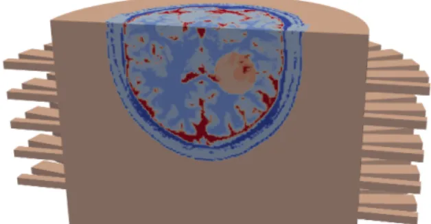
We use synthetic data corresponding to an accurate numerical model of a human head with a simulated hemorrhagic stroke as input for the inverse problem. The numerical model of the virtual head comes from CT and MRI scans and consists of a complex permittivity map of 362 × 434 × 362 data points with a spatial resolution of 500 µm. In the simulation, the head is immersed in the imaging chamber as shown in Fig. 9.

Fig. 9. Imaginary part of the relative complex permittivity of the virtual head model immersed in the imaging chamber with a simulated ellipsoid-shaped hemorrhagic stroke.

2) Reconstructions of a Hemorrhagic Stroke

In order to simulate the evolution of a hemorrhagic stroke, we use a synthetic ellipsoid-shaped stroke whose size (principal axes) increases over time, from 3.9 cm × 2.3 cm × 2.3 cm (small stroke) to 7.7 cm × 4.6 cm × 4.6 cm (large stroke). For this test case, the relative complex permittivity of the ellipsoid is assumed to be inhomogeneous where the relative complex permittivity at each quadrature point of the mesh is taken as the mean value between the original healthy brain permittivity values (baseline values) and the permittivity of blood (

ε

_rblood= 68 − i44) at f = 1 GHz. The imaging chamber is filled with the matching solution

_ε

_rmatching= 44 – i20. In a real experiment, a special membrane fitting the shape of the head is used in order to isolate the head from the matching medium (Fig. 3). We do not take this membrane into account in this synthetic test case. The synthetic data are obtained by solving the direct problem using a mesh composed of 17.6 million tetrahedra (corresponding to approximately 20 points per wavelength) and consist in the computed transmission and reflection coefficients

S

_ij. We subsequently add noise to the real and imaginary parts of the coefficients

S

_{ij (10% multiplicative} White Gaussian Noise (WGN)), with different values for real and imaginary parts, such as

S

_ijcorrupted

= S

ij

(1+10%AWGN )

(18) The corrupted data

S

_ijcorrupted are then used as input for the inverse problem. Furthermore, we do not assume any priori knowledge on the input data, and we set the initial guess for the inverse problem as the homogeneous matching solution everywhere inside the chamber. We use a piecewise linear approximation of the unknown parameter κ, defined on the same mesh used to solve the state and adjoint problems. For the purpose of parallel computations, the partitioning introduced by the domain decomposition method is also used to compute and store locally in each subdomain every entity involved in the inverse problem, such as the parameter κ and the gradient.

For Review Only

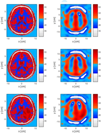
reconstructed relative permittivity, respectively, for the three

evolution steps of the hemorrhagic stroke, from a healthy brain, a brain with a small and large stroke. Increasing the size of the ellipsoid simulates the evolution of the stroke. Each reconstruction corresponds to the solution of an inverse problem in the truncated domain containing only the first two rings of antennas from the top. The transmitting antennas are on the first ring and receiving antennas on first and second rings. Therefore the scattering matrix contains only 64×32

S

_ij coefficients. Each reconstruction starts from an initial guess consisting of the homogeneous matching solution. The solution is obtained at about 30 iteration steps when reaching the convergence criterion of 10-2 _{for the value of the cost} functional using the L-BFGS algorithm.

Fig. 10. Transverse cross-section of the virtual brain during the evolution of a simulated hemorrhagic stroke: real part of the relative complex permittivity. Left: virtual brain model. Right: reconstructed permittivity. From top to bottom: healthy brain, brain with small stroke, brain with large stroke.

The evolution of the stroke can be visually monitored from the real and imaginary parts of the reconstructed complex permittivity. Nevertheless, the threshold to firmly conclude must only be determined from clinical studies on a large number of patients. One important point is to discriminate a hemorrhagic from an ischemic stroke. For this study case, the reconstructed values show an increase of the complex permittivity allowing the assumption of a hemorrhagic stroke versus an ischemic one.

Fig. 11. Transverse cross-section of the virtual brain during the evolution of a simulated hemorrhagic stroke: imaginary part of the relative permittivity. Left: virtual brain model. Right: reconstructed permittivity. From top to bottom: healthy brain, brain with small stroke, brain with large stroke.

The distribution of the relative error on the real and imaginary parts of the reconstructed complex permittivity for the small stroke case is shown in Fig. 12. We compute the relative error using (19) for each pixel (n,m) of the reconstructed relative complex permittivity. This error can be positive or negative.

err

_relative

(m,n) =

ε

r reconstructed

_{(m,n) −ε}

r exact

_(m,n)

ε

r exact

_(m,n)

(19)

We note that lowest errors are located outside the brain and in the stroke. This can be expected as the inversion algorithm performs better for homogeneous media such as the matching liquid but also for the stroke, as the complex permittivity value of the stroke is calculated as the mean value between the healthy tissues and the blood. This process tends to average the values, which is more favorable for the inversion algorithm. But, even if the brain is highly heterogeneous, the stroke can be detected and monitored with the proposed algorithm.

We now calculate the L2 norm of the error of the reconstructed images in such manner as (10). Results are shown in Table III. The L2 norm is interesting as it gives a global quantitative criterion for estimating the performance of the reconstructed values. The L2 _{norm confirms the results shown in Fig.12 for}

For Review Only

the small stroke. The error on the real part of the complex

relative permittivity is lower than on the imaginary part. It is of the order of 10% for the real part whereas it is about 20% for the imaginary part.

Fig. 12. Small stroke: Distribution of the relative error on the real (left) and imaginary (right) parts of the reconstructed complex permittivity. From top to bottom: healthy brain, brain with small stroke, brain with large stroke.

Relative Error Real part Imaginary Part

Healthy Brain 8.95% 20.74% With Small Stroke 8.92% 20.72% With Large Stroke 8.53% 18.92% Table III. Average error on the reconstructed values (real and imaginary parts of the complex permittivity).

Although we have shown in section IV B that high order edge elements are efficient when solving the direct problem with very high accuracy, the reconstructed images differ very slightly when using different discretization orders and mesh sizes in the inverse problem. It turns out for our study case that elements of degree r=1 with 10 pts/λ are sufficient for detecting the stroke.

Reconstructed images for each test case shown in Figs. 10 and 11 are obtained with a total computing time of less than 2 minutes (94 seconds for the large stroke case) using 4096 cores of Curie. These preliminary results are very encouraging as we are already able to achieve a satisfactory reconstruction time in the perspective of using such an imaging technique for monitoring. This allows clinicians to obtain almost

instantaneous images 24/7 or on demand. Although the reconstructed images do not feature the complex heterogeneities of the brain, which is in accordance with what we expect from microwave imaging methods, they allow the characterization of the stroke and its monitoring.

IX. CONCLUSION

The idea behind this work comes from the paradigm to develop a (portable/transportable) microwave imaging system whose raw data are wirelessly transferred to a HPC. The HPC machine will then compute the 3D image of the patient's brain. Once reconstructed, the image is quickly transmitted from the computing center to the hospital for stroke detection (including ischemic/hemorrhagic discrimination) and monitoring during treatment.

We have developed a tool that reconstructs a tomographic microwave image of the brain in 94 seconds on 4096 computing cores. This computational time corresponds to clinician acceptance for rapid diagnosis or medical monitoring at the hospital. These images were obtained from corrupted synthetic data from a very accurate model of the complex permittivity of the brain. To our knowledge, this is the first time that such a realistic study (operational acquisition device, highly accurate three-dimensional synthetic data, 10% noise) shows the feasibility of microwave imaging. This study has been possible by the use of massively parallel computers and facilitated by HPDDM and FreeFem++ tools that we developed. The next step will be the validation of these results on clinical data.

ACKNOWLEDGMENT

This work was granted access to the HPC resources of TGCC@CEA under the allocations 067519 and 2016-067730 made by GENCI.

Authors would like to thank the French National Research Agency (ANR) for their support.

REFERENCES

[1] R. Sacco, et al. “An updated definition of stroke for the 21st century: a statement for healthcare professionals from the American Heart Association/American Stroke Association,” Stroke, 44(7), pp. 2064-2069, July 2013.

[2] Intercollegiate Stroke Working Party. National clinical

guideline for stroke, 4th edition. London: Royal College of

Physicians, 2012.

[3] S. Wegener, “Neuroimaging of acute ischaemic stroke: current challenges,” European Medical Journal (EMJ), pp. 49-52, July 2014.

[4] S. Semenov, R. Svenson, V. Posukh, A. Nazarov, Y. Sizov, A. Bulyshev, A. Souvorov, W. Chen, J. Kassell, and G. Tatsis, “Dielectrical spectroscopy of canine myocardium during acute ischemia and hypoxia at frequency spectrum from 100 kHz to 6 GHz,” IEEE Trans. Med. Imag., Vol. 21, No.6, pp. 703-707, June 2002.

[5] S. Semenov, B. Seiser, E. Stoegmann, and E. Auff, “Electromagnetic tomography for brain imaging: from virtual

For Review Only

to human brain,” 2014 IEEE Conference on Antenna

Measurements & Applications (CAMA), Antibes Juan-les-Pins, 2014. Paper CAMA1162-SP132.4.pdf.

[6] F. Hecht, “New development in FreeFem++,” J. Numer.

Math., vol. 20, no. 3-4, pp. 251–265, 2012.

[7] J.-C. Nédélec, “Mixed finite elements in R3_{,” Numer.}

Math., vol. 35, no. 3, pp. 315–341, 1980.

[8] F. Rapetti, “High order edge elements on simplicial meshes,” M2AN Math. Model. Numer. Anal., vol. 41, no. 6, pp. 1001–1020, 2007.

[9] F. Rapetti, and A. Bossavit, “Whitney forms of higher degree,” SIAM J. Numer. Anal., vol. 47, no. 3, pp. 2369– 2386, 2009.

[10] M. Bonazzoli, V. Dolean, F. Rapetti, and P.-H. Tournier, “Parallel preconditioners for high order discretizations arising from full system modeling for brain microwave imaging,” Jun. 2016, preprint (available: https://hal.archives-ouvertes.fr/hal-01328197).

[11] P. Jolivet, V. Dolean, F. Hecht, F. Nataf, C. Prud’homme, and N. Spillane, “High-performance domain decomposition methods on massively parallel architectures with FreeFem++,”

Journal of Numerical Mathematics, vol. 20, no. 3-4, pp. 287–

302, 2012.

[12] P. Jolivet, F. Hecht, F. Nataf, and C. Prud’Homme, “Scalable domain decomposition preconditioners for heterogeneous elliptic problems,” in Proc. of the Int.

Conference on High Performance Computing, Network- ing, Storage and Analysis. IEEE, 2013, pp. 1–11.

[13] V. Dolean, P. Jolivet, and F. Nataf, An Introduction to

Domain Decomposition Methods: algorithms, theory and parallel implementation. SIAM, 2015.

[14] G. Karypis, and V. Kumar, “A fast and high quality multilevel scheme for partitioning irregular graphs,” SIAM

Journal on Scientific Computing, vol. 20, no. 1, pp. 359–392,

1998.

[15] X.-C. Cai, and M. Sarkis, “A restricted additive Schwarz preconditioner for general sparse linear systems,” SIAM J. Sci.

Comput., vol. 21, no. 2, pp. 792–797, 1999.

[16] V. Dolean, M. Gander, and L. Gerardo-Giorda, “Optimized Schwarz methods for Maxwell’s equations”,

SIAM J. Sci. Comput. 2009; vol. 31, no.3, 2193–2213.

[17] O. Schenk, and K. Gärtner, “Solving unsymmetric sparse systems of linear equations with PARDISO,” Future

Generation Computer Systems, vol. 20, pp. 3475–487, 2004.

[18] P. Amestoy, I. Duff, J.-Y. L’Excellent, and J. Koster, “A fully asynchronous multifrontal solver using distributed dynamic scheduling,” SIAM Journal on Matrix Analysis and Applications, vol. 23, no.1, pp.15–41, 2001.

[19] F. Pellegrini, and J. Roman, “SCOTCH: A software package for static mapping by dual recursive bipartitioning of process and architecture graphs, in High-Performance