HAL Id: hal-03195735
https://hal.archives-ouvertes.fr/hal-03195735
Submitted on 14 Apr 2021
HAL is a multi-disciplinary open access
archive for the deposit and dissemination of
sci-entific research documents, whether they are
pub-lished or not. The documents may come from
teaching and research institutions in France or
abroad, or from public or private research centers.
L’archive ouverte pluridisciplinaire HAL, est
destinée au dépôt et à la diffusion de documents
scientifiques de niveau recherche, publiés ou non,
émanant des établissements d’enseignement et de
recherche français ou étrangers, des laboratoires
publics ou privés.
Copyright
Log Data Preparation for Predicting Critical Errors
Occurrences
Myriam Lopez, Marie Beurton-Aimar, Gayo Diallo, Sofian Maabout
To cite this version:
Myriam Lopez, Marie Beurton-Aimar, Gayo Diallo, Sofian Maabout. Log Data Preparation for
Pre-dicting Critical Errors Occurrences. Trends and Applications in Information Systems and
Technolo-gies, 1366, pp.224-233, 2021, Advances in Intelligent Systems and Computing,
�10.1007/978-3-030-72651-5_22�. �hal-03195735�
Log Data Preparation for Predicting Critical
Errors Occurrences
Myriam Lopez1, Marie Beurton-Aimar1
Gayo Diallo1,2, Sofian Maabout1
1 University of Bordeaux, LaBRI, UMR 5800, Talence, France
{myriam.lopez, marie.beurton, sofian.maabout}@labri.fr
2 BPH INSERM 1219, Univ. of Bordeaux, F-33000, Bordeaux, France
Abstract. Failure anticipation is one of the key industrial research ob-jectives with the advent of Industry 4.0. This paper presents an approach to predict high importance errors using log data emitted by machine tools. It uses the concept of bag to summarize events provided by re-mote machines, available within log files. The idea of bag is inspired by the Multiple Instance Learning paradigm. However, our proposal follows a different strategy to label bags, that we wanted as simple as possible. Three main setting parameters are defined to build the training set allow-ing the model to fine-tune the trade-off between early warnallow-ing, historic informativeness and forecast accuracy. The effectiveness of the approach is demonstrated using a real industrial application where critical errors can be predicted up to seven days in advance thanks to a classification model.
Keywords: Predictive Maintenance (PdM), Machine Learning (ML), Classifi-cation, Log data, data preparation
1
Introduction
Predictive maintenance is of paramount importance for manufacturers ([6, 10]). Predicting failures allows anticipating machine maintenance and thus enabling financial saving thanks to shortening the off-period of a machine and anticipating the spare parts orders.
Nowadays, most modern machines in the manufacture domain are equipped with sensors which measure various physical properties such as oil pressure or coolant temperature. Any signal from these sensors is subsequently processed later in order to identify over time the indicators of abnormal operation ([12]). Once cleaned, historical data from sensors can be extremely valuable for predic-tion. Indeed, their richness makes it possible to visualize the state of the system over time in the form of a remaining useful life estimation ([5]).
In parallel, machines regularly deliver logs recording different events that enable tracking the conditions of use and abnormalities. Hence, event-based pre-diction is a key research topic in predictive maintenance ([13, 4]).
Our contribution in this paper is a data preparation approach whose output is used to learn a model for predicting errors/failures occurrences. It relies on the exploitation of historical log data associated to machines. The purpose is to predict sufficiently early the occurrence of a critical malfunction in the pur-pose of maintenance operations facilitation. The propur-posed framework is applied on a real industrial context and the empirical obtained performances show its effectiveness.
After introducing in the next section key definitions and parameters, we detail the data preparation process. Afterwards, we report on some of the experiments conducted in the context of our case study. Thereafter, we provide an overview of related work. Finally, we conclude and outline some indications for future work.
2
Dataset Collection and Preliminary Definitions
We suppose that we are given a log file F emitted by a machine M where the errors that have been observed by sensors associated to M are reported. We assume that the errors are logged in regular time intervals. Moreover, we consider a set of errors E = L ∪ H where L is the set of low errors `j and H is the
set of critical errors hj (high errors that will be called target in the following).
Our aim is to predict high errors wrt other errors. Each record in F is a pair hi, Ei where i is a timestamp expressed in days and E ∈ N|E| is a vector where
E[j] represents the number of occurrences of error ej∈ E at timestamp i. Hence,
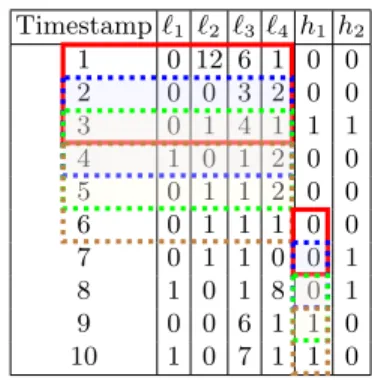
F is a temporal ordered sequence of such records. The following is the running example we use throughout the paper as an illustration of the approach. Example 1. Let the errors set be E = {`1, `2, `3, `4} ∪ {h1, h2} and consider the
following sequence (Table 1):
T imestamp `1 `2 `3 `4 h1 h2 1 0 12 6 1 0 0 2 0 0 3 2 0 0 3 0 1 4 1 1 1 4 1 0 1 2 0 0 5 0 1 1 2 0 0 6 0 1 1 1 0 0 7 0 1 1 0 0 1 8 1 0 1 8 0 1 9 0 0 6 1 1 0 10 1 0 7 1 1 0
Table 1: Example of a log event dataset with timestamp
For example, the first row/record whose timestamp is 1 says, among others, that at day 1, there have been 12 occurrences of low error `2and no occurrence
To come up with a prediction model and collect the data, three parameters, depicted in Figure 1, are applied :
– Predictive Interval : it describes the history of data used to perform pre-dictions and, its size in days is defined by the parameter P I. The information contained in that interval is gathered in a structure referred as a bag. – Responsive Interval : since, from a practical point of view, making a
prediction for the next day is of little interest, a common strategy is to constrain the model to forecast sufficiently early. The Responsive Interval is located immediately after the Predictive Interval and its size which controls how much early we want the model to forecast, is defined by the parameter RI.
– Error Interval : intuitively, this interval, whose size is defined by parameter EI, allows to make error occurrence prediction wrt a time interval instead of a time unit. It therefore introduces a degree of uncertainty of the prediction’s temporality.
Fig. 1: The key parameters of model prediction
Example 2. Let P I = 3, RI = 4 and EI = 2. With this setting, we want to predict high errors wrt bags of size 3, and this prediction concerns a period whose duration is 2 days starting 4 days after the end of the observed bag. More precisely, the fact that EI = 2 means that a predicted error occurrence may happen either at the first, the second, or both days within the error interval. Consider the bag B1defined between timestamps i = 1 and i = 3 in the Table 1.
Then the prediction period (Error Interval) concerned by B1 is in timestamp
[8, 9]. That is, at i = 3, we observe the bag B1 and we should be able to say
whether, or not, a high error will occur between i = 8 and i = 9.
3
Proposed Methodology
The current section describes how training and test sets are prepared. Indeed, in order to train a binary predictive model, a prerequisite is to build a training set where each sample is labeled YES/NO and corresponds to a situation where, respectively, a high error occurred or not.
Definition 1. Let Bi be a bag and given a target high error hj. Bi is labeled
YES iff time interval [i + P I + RI; i + P I + RI + EI − 1] contains an occurrence of hj. Bi is labeled NO otherwise.
Example 3. Let P I = 3, RI = 2 and EI = 2. Consider again the running ex-ample and let us focus on error h1. To decide the label of bag B1, we need to
check whether in [6; 7] error h1 has been observed. Since target has not been
observed, then B1takes label NO. Hence, referring to Table 1 and applying the
definition above, the bags B1and B2are labeled as NO and the bags B3and B4
are labeled as YES. Observe that since their corresponding EI period is outside the bounds of the available history, bags 5, 6, 7 and 8 cannot be labeled.
3.1 Summarization Strategy
The reader may notice that the above configuration (labeled bags) is close to the one encountered in the Multiple Instance Learning (MIL) [3]. However, our setting cannot be in conformance with MIL because the objective is a prediction based on the whole bag rather than individual samples. Thus, we choose an alternative approach, by summarizing every bag Bi by maximizing values and
transform it into a single features vector3.
Example 4. Let P I = 3 and consider the bag B1 starting at i = 1 and ending at
i = 3. The bag is summarized by the vector h0, 12, 6, 2i. That is, for each `j we
take the maximum of its values in B1. So, with RI = 2 and EI = 2 and when
considering the target error h1 we obtain the data set presented in Figure 2.
Timestamp `1 `2 `3 `4 h1 h2 1 0 12 6 1 0 0 2 0 0 3 2 0 0 3 0 1 4 1 1 1 4 1 0 1 2 0 0 5 0 1 1 2 0 0 6 0 1 1 1 0 0 7 0 1 1 0 0 1 8 1 0 1 8 0 1 9 0 0 6 1 1 0 10 1 0 7 1 1 0 Bag `1 `2 `3 `4 h2 Label h1 B1 0 12 6 2 1 NO B2 1 1 4 2 1 NO B3 1 1 4 2 1 YES B4 1 1 1 2 0 YES
Fig. 2: Bag summarization strategy by MAX() function
Each sample in the right pane of Figure 2 on one hand, is the total number of occurrences of every `j during a period of size P I = 3. The last columns testify
whether h1 has occurred (YES) or not (NO) after this period at a precise time
interval. The table on the left pane reminds the original data set.
3
Other methods of summarization can be used but in our use case, the MAX() function allowed us to obtain good prediction performances.
3.2 Overall Data Preparation Process
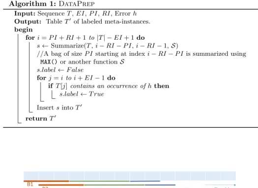
Figure 3 and Algorithm 1 depict our preprocessing stage. From a log file T , the consecutive records are gathered into bags using a sliding window of size P I. The label of each bag Bi depends on the content of interval EIi. The starting point
of EIi is RI time units after the end point of Bi. Once the bags are identified
and labeled, they are summarized by MAX() function to obtain the input data set T0 for model learning. As it may be seen from Algorithm 1, the complexity of data preparation is linear with the size of the sequence: the outer most loop is executed O(|T |) times. At each iteration, P I data rows are summarized and the label is assigned after checking EI row records. Hence, the overall complexity is O(|T |×(P I +EI)). From a computing point of view, the outer loop can be easily made parallel because the different iterations are independent of each others.
Algorithm 1: DataPrep
Input: Sequence T , EI, P I, RI, Error h Output: Table T0 of labeled meta-instances. begin
for i = P I + RI + 1 to |T | − EI + 1 do
s ← Summarize(T , i − RI − P I, i − RI − 1, S)
//A bag of size P I starting at index i − RI − P I is summarized using MAX() or another function S
s.label ← F alse
for j = i to i + EI − 1 do
if T [j] contains an occurrence of h then s.label ← T rue
Insert s into T0 return T0
Fig. 3: Data Preparation Process. The bags of the training set are built by sliding windows with the following model parameters: P I = 3; RI = 4; EI = 2
4
Experiments
4.1 Dataset Description
We collected raw data from a one-year history of several log files. Each file is associated to a specific machine. All machines belong to the same model4. However, they are not subject to the same conditions of use. Given a combination of parameters (P I; RI; EI), each log file is processed using Algorithm 1. Output files are then merged to constitute our input dataset. The latter is partitioned into a 80/20 ratio of training and test sets respectively. The partitioning relies on a stratified sampling to keep a similar proportion of positive samples both in the test and training sets.
The dataset contains 193 features (i.e., distinct low errors) and 26 high errors (our targets). For every high error, we designed several models, each of which is obtained by combination of three parameter values (P I; RI; EI). As part of our study, we were interested in the 11 most frequent target errors which occur in the dataset. Depending on the target, we ended up with an average of 1000 samples, among which, from 4% to 30% are positive. Although a balance correction technique is in general recommended in such a case, our experiments showed that subsampling did not provide any substantial accurracy gain5. Then,
we decided not to make use of subsampling.
In the following experiments the default value for both parameters P I and RI is 7 days. The value of the RI parameter is chosen as constraint because the idea is that the model anticipates 7 days before the error target occurs.
4.2 Settings
All experiments were conducted with the RapidMiner software6. Several classi-fier algorithms were explored, e.g., SVM, Naive Bayes, Random Forest, Decision Tree and the multi-layer feed-forward artificial neural network (NN) algorithm of the H2o framework [1]. NN algorithm outperformed the others and was sub-sequentely chosen as the actual predictive model. Experiments were set with 4 layers of 100 neurons each, 1000 epochs and a Cross Entropy loss function for the learning phase.
To assess the performance of a prediction model, different metrics can be used. Among these, Accuracy and F1-score are suitable one. Accuracy is the ratio of correct predictions. F1-score wrt to the positive class is given by the harmonic mean of precision and recall7:
2(precision × recall) (precision + recall) =
2 × T P
2 × T P + F P + F N (1)
4
Regretfully, for confidentiality reasons we cannot share the data used for this study
5
Due to lack of space the results will not be detailed in this paper.
6 Rapidminer.com 7 precision= T P T P +F P and recall= T P T P +F N.
T P , T N , F P , F N represent respectively, true positives, true negatives, false positives and false negatives. Because negative cases are much more frequent than positive one, accuracy alone is not sufficient to assess the performance of the model. F1-score allows to observe in more details the behavior of the model regarding the class of interest, in our case, the positive one.
4.3 Impact of the Error Interval Choice
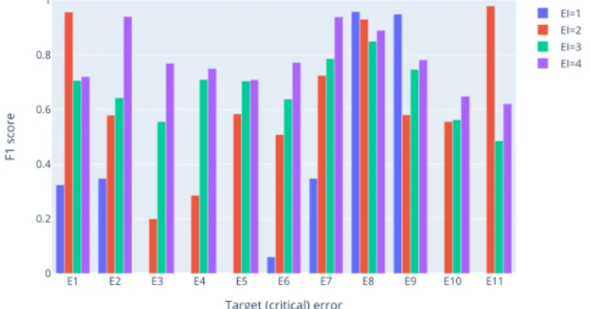
Parameter EI introduces a flexibility wrt positive predictions as well as a rigidity for negative ones. Indeed, a positive prediction says that at some point in a future time interval, a high error may occur while a negative prediction says, no occurrence at any point in a future time interval. Intuitively and regarding positive predictions, one may expect that the higher EI, the more correct the model’s predictions are. To analyse this hypothesis we varied EI from 1 to 4 days and for each target error, we computed F1-score wrt the positive class8
The obtained results are depicted in Figure 4.
Fig. 4: F1-score evolution wrt EI
Overall, our initial assumption is confirmed. We observe that for about half of the errors, setting EI to 1 day leads to a significant degradation of the model’s performance. In these cases the model yields to F1 score equal to zero (see errors E3 ; E4 ; E5 ; E10 and E11) explained by a null value of true positive prediction. For E8 and E9, the results show a different phenomenon from overall behaviour. Indeed, the largest F1 score for these errors is obtained when EI is set to 1.
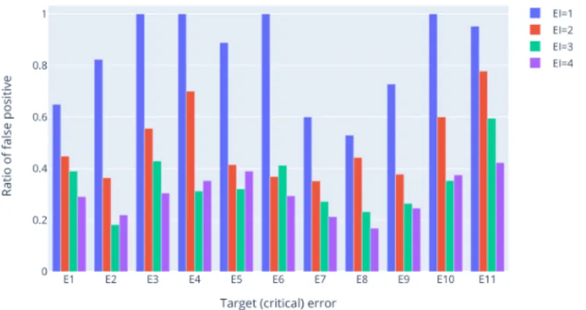
F1-score gives a global picture of the predictive model behavior wrt positive class in that it combines precision and recall measures. From the application perspective, false alarms, i.e., false positives ratio (F P R) is a key indicator9.
8 Due to space limitation, we do not present here the prediction for negative class. 9
F P R = F P
Fig. 5: False positive (false alarm) ratio wrt EI
Figure 5 shows the evolution of F P R with respect to EI. We observe that in general, increasing EI tends to decrease F P R, hence it increases the precision. Increasing the size of the EI concomitantly increases the number of positives examples in the training dataset. That can explain that we obtained better performances with a greater EI. Although these performances may also in some cases mask an over-expression of false positives, the phenomenom is not present here, as proven in Figure 5.
Despite the general trend of F1-score and precision wrt EI, the model per-formance is not monotonic. For example, the learned model for error E1 has the highest F1-score when EI = 2. This indicates that for every error, one needs to calibrate the most convenient EI regarding applications/F1-score needs.
5
Related Work
Fault anticipation for predictive maintenance has attracted a large body of re-search (please see e.g., recent surveys [9, 8, 14]) and several paradigms have been used for this purpose. Our solution belongs to the class of approaches based on supervised machine learning. As such, we focus our comparison to these tech-niques and more specifically on [11] and [7] that are, to our knowledge, the closest previous works.
Let us start with [11]. Despite some subtle differences, the task of tagging the bags as negative or positive instances is similar to that of [11]. However, in the latter, negative bags propagate their label to each individual instance belonging to them. By contrast, every positive bag is aggregated using the average measure and gives rise to a new positive meta-instance. Therefore, the training data set is a mix of meta-instances (positive in this case) and simple instances (negative ones). The rational behind the use of the average score is that the so obtained instance is considered as a representative of a daily behavior inside a bag. In fact, and unless having a small standard deviation inside positive bags, a daily
record can be very different from the average of the bag it belongs to. Hence learning from bag averages and predicting from single instances may present some discrepancy. The data for our case study present high deviations inside the bags, which makes it hopeless to identify positive records using averaged records. In our case, the data preparation process considers positive and negative bags equally. In that way, consider the occurrence or not of a high error/failure is explained by the whole bag associated to it, and not just some instances belonging to that bag. Moreover, in contrast to what has been suggested in the work of [11], this way of proceeding reduces the issue of unbalanced classes that we are confronted with.
Now let us consider the prediction phase. In [11], prediction is instance based (i.e., daily records) and these predictions are then propagated to bags. More precisely, during the prediction phase, successive instances belonging to the un-classified bag, are provided to the learned model. If one of them is un-classified as positive then the whole bag is positive. It is negative otherwise10. So
funda-mentally, predictions are daily based in the sense that the real explanation of a possible error/failure occurrence depends actually on what happens during a day while ours needs are to combine events of larger intervals. This is also the reason why, unlike [11], our work is not in conformance with Multi-Instance Learning paradigm (MIL). Indeed, the MIL main hypothesis states that a bag is positive iff one of its instances is positive [3, 2], while our approach does not impose any condition on individual instances. We have applied the methodology of [11] over our use case, but could not obtain F1-score better than 0.2.
A more recent work with a similar data preparation process as [11] is [7]. The main difference is that its learned model is a regression that estimates the probability of a future error occurrence. If this probability is higher than some fixed threshold, then an alert is fired. Hence, during data preparation, the labels associated to bags are probabilities instead of YES/NO labels. Intuitively, the closer a bag is to an error, the higher is its probability. To handle this property, the authors used a sigmoid function. The reported results show that the proposed techniques outperform those of [11] by a large margin. We believe that this is mainly due to the data nature defining the use case and in general there is no absolute winner. As it has been shown in the experiments, our targeted use case does not need such complex techniques to achieve high prediction accuracy.
6
Conclusion and Future Works
We described an approach to exploit log data for predicting critical errors that may cause costly failures in the industry manufacture domain. The approach is based on aggregation of temporal intervals that precede these errors. Combined with a neural network, our solution turns to be highly accurate. Its main advan-tage, compared to other techniques, is its simplicity. Even if we do not claim that
10Notice that in [11], during data preparation, bags are first labeled and then, their
labels are propagated to instances while for bag label prediction, the labels of its instances are first predicted and then the bag label is deduced.
it should work for every similar setting (log based prediction), we argue that it could be considered as a baseline before trying more sophisticated options. We applied our solution to a real industrial use case where a dozen of highly criti-cal errors were to be predicted. The obtained accuracy and F1-score belong to respectively [0.8; 0.95], and [0.6; 0.9] which can be considered as highly effective compared to the reported results on log based failures prediction litterature.
So far, we designed one model per target error. In the future, we plan to analyze in more depth the errors to see whether it would be possible to combine different predictions in order to reduce the number of models. In addition, we are interested in automating the parameters setting: given a (set of) target(s), to find the optimal values of P I, EI and RI such that the learned model performances is maximized.
References
1. Candel, A., Parmar, V., LeDell, E., Arora, A.: Deep learning with H2O (2016), h2O AI Inc
2. Carbonneau, M., Cheplygina, V., Granger, E., Gagnon, G.: Multiple instance learn-ing: A survey of problem characteristics and applications. Pattern Recognit. 77, 329–353 (2018)
3. Dietterich, T.G., Lathrop, R.H., Lozano-P´erez, T.: Solving the multiple in-stance problem with axis-parallel rectangles. Artif. Intell. 89(1-2), 31–71 (1997), https://doi.org/10.1016/S0004-3702(96)00034-3
4. Gmati, F.E., Chakhar, S., Chaari, W.L., Xu, M.: A Taxonomy of Event Prediction Methods. In: Proc. of IEA/AIE conf. Springer (2019)
5. Guo, L., Li, N., Jia, F., Lei, Y., Lin, J.: A recurrent neural network based health indicator for remaining useful life prediction of bearings. Neurocomputing 240, 98–109 (2017)
6. Hashemian, H.M.: State-of-the-art predictive maintenance techniques. IEEE Trans. Instrum. Meas. 60(1), 226–236 (2011)
7. Korvesis, P., Besseau, S., Vazirgiannis, M.: Predictive maintenance in aviation: Failure prediction from post-flight reports. In: Proc. of ICDE Conf. (2018) 8. Krupitzer, C., Wagenhals, T., Z¨ufle, M., et al.: A survey on predictive maintenance
for industry 4.0. CoRR abs/2002.08224 (2020)
9. Ran, Y., Zhou, X., Lin, P., Wen, Y., Deng, R.: A survey of predictive maintenance: Systems, purposes and approaches. CoRR abs/1912.07383 (2019)
10. Salfner, F., Lenk, M., Malek, M.: A survey of online failure prediction methods. ACM Comput. Surv. 42(3), 10:1–10:42 (2010)
11. Sipos, R., Fradkin, D., M¨orchen, F., Wang, Z.: Log-based predictive maintenance. In: SIGKDD conference. pp. 1867–1876. ACM (2014)
12. Wang, C., Vo, H.T., Ni, P.: An iot application for fault diagnosis and prediction. In: IEEE International Conference on Data Science and Data Intensive Systems. pp. 726–731 (2015)
13. Wang, J., Li, C., Han, S., Sarkar, S., Zhou, X.: Predictive maintenance based on event-log analysis: A case study. IBM J. Res. Dev. 61(1), 11 (2017)
14. Zhang, W., Yang, D., Wang, H.: Data-driven methods for predictive maintenance of industrial equipment: A survey. IEEE Systems Journal 13(3), 2213–2227 (2019)