HAL Id: inria-00278553
https://hal.inria.fr/inria-00278553v2
Submitted on 14 May 2008
HAL is a multi-disciplinary open access
archive for the deposit and dissemination of
sci-L’archive ouverte pluridisciplinaire HAL, est
destinée au dépôt et à la diffusion de documents
mammalian chromosomes
Claire Lemaitre, Eric Tannier, Christian Gautier, Marie-France Sagot
To cite this version:
Claire Lemaitre, Eric Tannier, Christian Gautier, Marie-France Sagot. Precise detection of
rearrange-ment breakpoints in mammalian chromosomes. [Research Report] RR-6533, INRIA. 2008, pp.26.
�inria-00278553v2�
inria-00278553, version 2 - 14 May 2008
a p p o r t
d e r e c h e r c h e
3 9 9 IS R N IN R IA /R R --6 5 3 3 --F R + E N G Thème BIOPrecise detection of rearrangement breakpoints in
mammalian chromosomes
Claire Lemaitre — Eric Tannier — Christian Gautier — Marie-France Sagot
N° 6533
mammalian chromosomes
Claire Lemaitre
∗†, Eric Tannier
†, Christian Gautier
†, Marie-France Sagot
†Th`eme BIO — Syst`emes biologiques Projet Helix
Rapport de recherche n°6533 — Mai 2008 — 26 pages
Abstract: Genomes undergo large structural changes that alter their organisation. The chromosomal regions affected by these rearrangements are called breakpoints, while those which have not been rearranged are called synteny blocks. We developed a method to pre-cisely locate rearrangement breakpoints on a genome by comparison with the genome of a related species. Contrary to current methods which search for synteny blocks and simply return what remains in the genome as breakpoints, we propose to investigate the breakpoints themselves in order to refine them. By aligning each breakpoint sequence against its specific orthologous sequences in the other species, we can look for weak similarity inside the break-point, thus extending the synteny blocks and narrowing the breakpoints. The identification of the narrowed breakpoints relies on a segmentation algorithm and is statistically assessed. Since this method requires as input synteny blocks with some properties which, though they appear natural, are not verified by current methods for detecting such blocks, we further give a formal definition and provide an algorithm to compute them. The whole method is applied to locate breakpoints on the human genome when compared to the mouse and dog genomes. Among the 355 human-mouse and 240 human-dog breakpoints, 168 and 146 respectively span less than 50 Kb. We compared the resulting breakpoints with some pub-licly available ones and show that we achieve a better resolution. Furthermore, we suggest that breakpoints are rarely reduced to a point, and instead consist in often large regions that can be distinguished from the sequences around in terms of segmental duplications, similarity with related species, and transposable elements. We hope that this new result may provide some insight into the mechanism and evolutionary properties of chromosomal rearrangements.
Key-words: rearrangement, genome dynamics, genome evolution, breakpoint analysis
∗clemaitr@biomserv.univ-lyon1.fr
†Universit´e de Lyon, F-69000, Lyon ; Universit´e Lyon 1 ; CNRS, UMR5558, Laboratoire de Biom´etrie
et Biologie Evolutive, F-69622, Villeurbanne, France.
Projet Helix, INRIA Rhˆone-Alpes, 655 avenue de l’Europe, 38330 Montbonnot Saint-Martin, FranceShared foot note
dans les g´
enomes de mammif`
eres
R´esum´e : Les g´enomes ´evoluent par mutations ponctuelles et par des modifications `a plus grande ´echelle qui alt`erent leur organisation. Les r´egions g´enomiques affect´ees par ces r´earrangements sont appel´ees points de cassure, alors que celles qui n’ont subit aucun r´earrangement sont appel´ees blocs de synt´enie. Nous avons d´evelopp´e une m´ethode pour d´etecter pr´ecis´ement les points de cassure sur un g´enome, par comparaison avec un g´enome d’une esp`ece proche. Contrairement aux m´ethodes actuelles qui cherchent les blocs de synt´enie et identifient les points de cassure simplement par les r´egions restantes, nous proposons de nous concentrer sur chaque point de cassure pour le raffiner. En alignant chaque s´equence de point de cassure avec ses s´equences orthologues dans l’autre g´enome, nous pouvons d´etecter des similarit´es faibles, permettant d’´etendre les limites des blocs de synt´enie. L’identification des limites du point de cassure est effectu´ee par un algorithme de segmentation et est ensuite ´evalu´ee statistiquement. Cette m´ethode impose certaines propri´et´es aux blocs de synt´enie, qui, bien que naturelles, ne sont pas respect´ees par les m´ethodes actuelles. Nous proposons, alors, une d´efinition formelle des blocs de synt´enie et donnons un algorithme pour les calculer. La m´ethode est appliqu´ee afin d’identifier les points de cassure sur le g´enome humain, compar´e avec ceux de la souris et du chien. Parmi les 355 points de cassures homme-souris et les 240 homme-chien, 168 et 146 respectivement sont r´eduits `a moins de 50 Kb. Nous avons compar´e nos r´esultats avec des donn´ees publi´ees, et nous montrons que nous obtenons une meilleure r´esolution. De plus, nous observons que les points de cassure sont rarement r´eduits `a un point, mais, au contraire, constituent une r´egion ´etendue qui se diff´erencie des r´egions voisines en termes de duplications segmentaires, de similarit´e avec des esp`eces proches et d’´el´ements transposables. Nous esp´erons que ces nouveaux r´esultats permettront de mieux comprendre les m´ecanismes et les propri´et´es ´evolutives des r´earrangements chromosomiques.
1
Introduction
Rearrangements are large scale modifications of the genome that can occur after a double-strand break of the DNA molecule if the latter is mis-repaired. They can correspond to inversions or transpositions of DNA segments, translocations between non homologous chro-mosomes, fusions or fissions of chrochro-mosomes, deletions or duplications of small or large por-tions. Such modifications in the organisation of a genome are not without consequences for the cell and the organism. As a matter of fact, rearrangements have been shown to be responsible for numerous heritable diseases, called genomic disorders. They are further involved in evolution, speciation, and also in cancer (for reviews on all these topics see [1, 14, 29, 33]). Although they have been studied for a long time, the underlying mecha-nisms of such events remain largely unknown, in particular understanding (predicting) their location on the genome. As far as evolutionary rearrangements are concerned, it thus re-mains an open question to understand what determines their locations. Whereas Nadeau and Taylor suggested in 1984 that rearrangements occur randomly on a genome [24], sev-eral observations tend to refute this model and suggest a more deterministic scenario. By comparing genomes of related species, it has thus been suggested that some rearrangements cluster in specific regions, called hotspots [8, 27]. A few rearrangement locations have also been found re-used in independent lineages in the course of evolution, indicating again that some regions seem to be more prone to a rearrangement than others [17, 22, 23]. In addition, several genomic features, such as segmental duplications or fragile sites, seem to correlate with rearrangement locations [2, 4, 30]. However, the nature of the relationship between such features and rearrangements, that is, whether one is a cause or a consequence of the other, remains unknown.
Of the numerous possible sources of structural variation due to a rearrangement, we deal only with those involving chromosomal regions above a certain size in number of markers (such as genes). The main motivation is that this decreases the risk of false positives, that is, of identifying regions as rearranged while they in fact have been detected as such following a wrong homology assignment. In practice, this means also that we do not deal with duplication or deletion events as those are harder to detect or to properly assign.
One crucial step before analysing the rearrangements and their possible relation with other genomic features is to locate these events on a genome. In the case of two genomes, it is possible to identify conserved regions by comparing the order and orientation of orthologous markers along the genomes. Conserved regions correspond to pairs of segments, one in each genome, that are orthologous and have not been rearranged in either lineage. These are also called synteny blocks. Breakpoint regions, or breakpoints for short, are segments that flank the conserved regions. More precisely, a breakpoint is the region between two consecutive synteny blocks on one genome, whose orthologous blocks are rearranged in the other genome (not consecutive or not in the same relative orientations).
A terminological clarification is called for here as the use of the term “breakpoint” to name such rearranged regions can be confusing for two reasons.
The first reason originates from the prefix “break”. This suggests a physical break of the DNA (such as a double strand break), and assigns an improper biological meaning to
the term. Indeed, the definition of breakpoints is based only on the method developed to identify it. One should therefore be aware that the so-called breakpoint regions have not necessarily been “broken”. The region we call breakpoint is located on one genome, and when comparing two genomes, we can usually not decide in which lineage the rearrangement in fact occurred. Suppose for instance that we are comparing the genomes of human and mouse and that the ancestral arrangement of one of the chromosomes is composed of the consecutive synteny blocks A, B and C. Suppose now that the human arrangement is the same as the ancestral one, ABC, and that the mouse arrangement is ACB. Then, by comparing the human and mouse genomes, the region between A and C in the mouse genome would appear as a breakpoint, as would the region between A and B in the human genome. However, neither of these two regions contain the real breakpoint (which is between Aand B in a mouse ancestor), but both are homologous to a broken region.
The second reason why the term “breakpoint” may be confusing originates from its suffix “point”. Indeed, most often the location of a breakpoint is not as precise as a point, that is as the position between two nucleotides on a genomic sequence. It concerns rather in general a longer region. This latter is defined as the region between two successive synteny blocks, implying that we have not detected any homology (modelled as a statistically significant enough similarity) for the region to be added to a neighbouring synteny block, or for it to be considered as a new block in itself. However, we do not know a priori if this imprecision is due to a genomic disorder created by (or explaining) the break (either the rearrangement itself affects a large region, or many other structural variations occurred before or after the rearrangement in the same region), or to the fact that it is computationally difficult to extend the orthology beyond the extremities of the synteny blocks.
Keeping these considerations in mind, we continue calling such regions breakpoints, for short.
We are interested in investigating such breakpoints more in detail. Indeed, in order to analyse the breakpoint sequence and to determine whether breakpoints correlate with some other features of the genome, it is important to precisely locate them. As far as we know, current methods for detecting breakpoints are in fact methods for detecting synteny blocks: they provide the coordinates of the breakpoints only as a byproduct, simply by returning regions that are not found in a conserved synteny. We propose here to go one step further and to extend the synteny blocks by focusing on the breakpoints themselves. It has been previously observed that inside breakpoints, one can often find some smaller blocks of weak similarity that could have been included in the original synteny blocks [35]. We have developed a formal method to precisely locate the breakpoints on a sequenced genome by a comparative approach with related species. Given two genomes, one of which will serve as reference, the core of the method assumes that some synteny blocks have been correctly identified. These delimit regions that are breakpoints but that can be refined in the sense that the blocks could be extended. Thus the regions between which there is no detectable orthology, that is the breakpoints, could be far more precisely and narrowly localised.
The method requires that the synteny blocks given as input do not overlap and that their extremities correspond to orthologous sequences between both species. Various methods
exist to construct synteny blocks from homologous markers between two sequences, but formal descriptions of these objects are rarer, and no current method can guarantee the simple properties we require. We thus describe our own method to build reliable and formally well described synteny blocks, for which we can guarantee the useful properties.
The method was then applied to mammalian genomic data. The human genome was chosen as reference and compared to two other mammalian genomes: those of the mouse and dog. We end up with a dataset of precise coordinates of mammalian breakpoints on the human genome, which is made publicly available. By comparison with other published datasets of breakpoint coordinates, we further show that in general, one can extend syn-teny blocks and refine breakpoints in an efficient enough manner. Finally, we analysed the breakpoint sequences in terms of several genomic features. This identifies some duplications inside the breakpoints and reveals differences with the flanking sequences.
2
Method
2.1
Refining the breakpoints
We start by describing the core of the method, that is the narrowing down as precisely as possible into the breakpoints given a set of synteny blocks.
We are given two sequenced genomes, and the synteny blocks between them. Since we wish to locate all the breakpoints in one genome, the method is not symmetric: one genome is thus the reference and is denoted by Gr, while the other genome to which it is compared
is denoted by Go. A synteny block is defined by a pair (Ar, Ao) of coordinates, one (Ar)
in genome Gr and the other (Ao) in genome Go, each indicating a chromosome, a start
point and an end point. A breakpoint on Gris a region between two synteny blocks that are
consecutive on Gr, but not on Go. Assuming that the synteny blocks are correct, it is certain
that in this region, or in one of its orthologs on the other genome, there has been at least one break due to a rearrangement. The size of the region can vary from several base pairs to several millions of base pairs. As mentioned in introduction, we do not know a priori if this imprecision is due to a biological property of the region, or to the fact that orthology has not been detected beyond the extremities of the synteny blocks. We are interested in refining this region as much as possible to eliminate the latter possibility. The refinement of the region is done by aligning the region in-between the two synteny blocks in Gr with
the regions flanking the orthologs of the blocks in Go. The results of the alignment are then
coded into a numerical sequence which is partitioned to identify the narrowed breakpoint.
2.1.1 Alignment
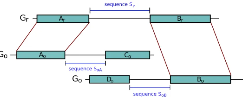
Given two synteny blocks (Ar, Ao) and (Br, Bo) that are consecutive in Gr, three sequences
of interest are defined (see Figure 1): Sr corresponds to the region in Gr between Ar and
Br, SoA and SoB are the sequences flanking Ao and Bo in Go (respecting the orientation)
Figure 1: An example of a breakpoint. The synteny blocks (Ar,Ao) and (Br,Bo) are
con-secutive on genome Gr but not on Go. It defines a breakpoint on Gr between the two
blocks. The sequence of the breakpoint is called sequence Sr. We define also sequence SoA
which flanks block (Ar,Ao) on Go and is bordered by the next block (Cr,Co) on Go. The
sequence SoB is defined similarly, flanking block (Br,Bo) on Go and bordered by the next
block (Dr,Do) on Go.
and SoB is expected to be orthologous to sequence Sr. As an example, in Figure 1, the
prefix of sequence Sr should be orthologous to the prefix of sequence SoA and its suffix to
the suffix of sequence SoB. Depending on the nature of the markers, their extremities may
be poorly conserved and the limits of the synteny blocks thus not very clear. The markers at the extremities of the blocks may then be added to the sequences Sr, SoA, and SoB. For
example, in the case of genes, when their orthology relationship has been assigned based on similarity criteria at the aminoacid level, the orthologous genes may not be alignable on their whole length at the DNA level and thus the extremities of the genes on the genomes may not be orthologous. This can also be due to errors in the prediction of the boundaries of genes. Including the genes at the extremities of the blocks in the sequences thus allows to overcome these problems.
To identify the orthologous relationships between sequence Sr and the two sequences
SoA and SoB, we perform two local alignments: one of sequence Sr against sequence SoA
and another of sequence Sragainst sequence SoB. We use for this the algorithm Blastz [31],
after having masked the sequences for repeats with RepeatMasker1. The choice of a local
aligner like Blastz is motivated by the fact that the sequences are usually (for the major part) intergenic, and therefore in general not well conserved over their whole length, and Blastz has been shown to be more sensitive on such sequences [31]. Large indels, small rearrangements and duplications are possible. The sequences are also often long. These two characteristics call for an algorithm that is both sensitive and fast enough.
Two lists of local alignments, called hits, are obtained and mapped onto sequence Sr,
regardless of their orientations and locations in the sequences SoA and SoB. We expect to
have significantly more hits from SoA in sequence Sr close to block Ar, and more hits from
sequence SoB close to Br. In the region in between, in general no clear difference can be
made between the amount of hits from SoA and SoB. This defines the refined breakpoint.
2.1.2 Segmentation
To detect this region in a quantitative manner, the information provided by the hits is coded along the sequence Srgiving as result a sequence I of discrete values of which three only are
possible: -1, 0 and 1. The value is 1 (resp. -1) if position i of Sr is covered by at least one
hit from sequence SoA (resp. SoB) and no hit from sequence SoB (resp. SoA). The value
is zero if position i is covered by at least one hit from each of the sequences SoA and SoB.
The positions covered by no hits are deleted from sequence I. Thus sequence I has length n, the number of positions covered by at least one hit.
The problem we solve is then, given the sequence I of -1, 0 and 1’s, to find the optimal segmentation of I into three segments, such that the first presents an orthology relationship with sequence SoA, the third segment an orthology relationship with sequence SoB, and the
segment in between corresponds to the breakpoint. We define two change points u1 and u2
over the sequence I of length n, such that 1 ≤ u1≤ u2≤ n. The sequence is modelled by a
piecewise constant function with the values µ1, µ2and µ3respectively in the three segments.
We are looking for the two change points u1and u2that minimise the sum of the squares
of the deviations of the data to the model (called the objective function): f(u1, u2) = 3 X j=1 uj X k=uj−1+1 (Ik− µj)2, with u0= 0 and u3= n. (1)
The values of µ1, µ2 and µ3 are defined as follows :
µ1= (Pu1 k=1Ik u1 if Pu1 k=1Ik>0 ∞ otherwise µ2= 0 µ3= (Pn k=u2+1Ik n−u2 if Pn k=u2+1Ik <0 ∞ otherwise
In the middle segment, µ2 equals zero, thus representing the breakpoint. In the two
extreme segments the value of the function is the observed mean of I over the segment if the latter has the “correct sign”. In order for the first (resp. last) segment to represent an orthology relationship with sequence SoA (resp. SoB), the value of the function must be
positive (resp. negative) meaning that it contains more hits with SoAthan with SoB (resp.
with SoB than with SoA). If the observed mean in the segment has the wrong sign, the
value is infinite; it ensures that this segment will not be part of the optimal solution since the contributions over this segment will be infinite.
Observe also that u1can be equal to 0, or to u2, and u2can be equal to n. This provides
the possibility for some segments to be empty, and thus to segment sequence I in less than 3 segments.
Since the objective function is additive over the contributions of the positions, a dynamic programming algorithm efficiently provides the optimal partition [3, 5]. Notice that, since the number of change points is two, a simple algorithm scanning all possible partitions would be as efficient: the execution time grows with the square of the length n of sequence I.
2.1.3 Speed-up
The problem we solve is, however, more constrained than the classical change-point detection problem. We show that the two change points u1 and u2 can be found independently in
linear time with the length of sequence I instead of using the classical dynamic programming algorithm in O(n2).
Lemma 1. Given the sequence I of size n, such that for all k ∈ {1, n}, Ik∈ {−1, 0, 1}, the
positions u1 and u2, with u1 ≤ u2, that minimise the function f (u1, u2) (see Formula (1))
are such that:
1 √u1 Pu1 k=1Ik is maximal, 1 √n−u2 Pn k=u2+1Ik is minimal.
Proof: First, by developing the square terms of each sum in function (1), we obtain: f(u1, u2) = n X k=1 I2 k − 1 u1 ( u1 X k=1 Ik)2− 1 n− u2 ( n X k=u2+1 Ik)2
The first term is a constant and the other two are independent from each other. Thus f(u1, u2) is minimal when the two last sums are both maximal, that is when S1(u1) =
1 √u1
Pu1
k=1Ik is maximal (since it must be positive), and S2(u2) = √n1 −u2
Pn
k=u2+1Ik is minimal (since it must be negative). However the solution must respect the condition u1≤ u2. We show next that this condition is always fulfilled.
Let x1 (resp. x2) be the position on I that maximises S1(u1) (resp. minimises S2(u2)).
Suppose x1> x2. Then: S1(x1) = √x1 1 Px1 k=1Ik= 1 √x1 Px2 k=1Ik+ 1 √x1 Px1 k=x2+1Ik S2(x2) = √n1 −x2 Pn k=x2+1Ik = 1 √n−x2 Px1 k=x2+1Ik+ 1 √n−x2 Pn k=x1+1Ik if Px1 k=x2+1Ik ≥ 0, then S2(x2) ≥ 1 √n−x2 Pn k=x1+1Ik > 1 √n−x1 Pn k=x1+1Ik = S2(x1), thus S2(x2) is not minimal.
else ( Px1 k=x2+1Ik <0), S1(x1) < 1 √x1 Px2 k=1Ik < 1 √x2 Px2 k=1Ik = S1(x2), thus S1(x1) is not maximal.
2.1.4 Statistical test
Whatever the structure of the signal, the method will output the best segmentation of the data into at most three segments. It is therefore important to test if the data are actually structured into three segments, respecting the constraints mentioned above, or if there is no such structure in sequence I. In the latter case, the obtained change points do not make statistical sense and we must conclude that we are not able to refine the breakpoint based on the alignments.
The more a given sequence I of length n is structured into three segments, the lower will be the value of the minimised objective function (that is the sum of the squares of the deviations of the data to the model), and thus the better will be the quality of the fit. What we need to test is therefore whether this fit is significantly better than the one that could be obtained with a non-structured sequence.
The null model is obtained by shuffling sequence I and computing for each permutation the value of the objective function corresponding to an optimal segmentation. Since I represents the alignment hits, the positions are not independent from one another and the values of 1 and -1 (corresponding to such hits) appear clustered. To take into account this structure in the shuffling operation, we do not shuffle individual positions, but instead blocks of consecutive identical values, given by the extremities of the hits. We accept the null hypothesis that I is not structured if more than five percent of the random permutations have a value that is lower than the value obtained by I.
2.2
Building the synteny blocks
2.2.1 Motivation
We now describe our own method for finding the synteny blocks. The general goal of such a method is to detect unbroken chains of markers which appear in the same order and same orientation in both genomes. Depending on the nature of the markers however, the orthologous relationships can be more or less reliable, and some errors or misleading relationships may disrupt regions of conserved order and orientation. This is why in general more flexible blocks of synteny are constructed.
Methods for identifying orthologous markers and for constructing synteny blocks are numerous in the scientific literature, starting with blocks built from physical or genetic maps of the chromosomes [13], to conserved segments of genes or blocks grouping genomic markers from whole genomic alignments [6, 9, 11, 12, 15, 16, 20, 25, 26, 32, 34]. The method to refine breakpoints described in the previous section requires two properties of the synteny blocks. First, they must not overlap on one or the other genome because this would lead to non-existing sequences Sr, SoA or SoB since the latter are defined as the sequences that
stand between two consecutive blocks. Second, the extremities of the synteny blocks must correspond to an orthology because they are used to define the sequences that will then be aligned. For example, in a block (Ar, Ao), the sequence at one extremity of Ar should be
Few methods for finding blocks available in the literature satisfy these requirements, and those that do so are either very computer intensive or are incompletely described heuristics. For example, GRIMM-synteny [26] builds blocks by clustering markers that are close to-gether, and keeps among the maximal clusters thus detected only those that are bigger than a threshold. The synteny blocks built by GRIMM-synteny may thus overlap. Furthermore, since markers are clustered based on a distance criterion regardless of their order and orien-tation, the boundaries of a synteny block on any of the two genomes may be defined by two markers which are not orthologous. For instance, in the example of Figure 2, the synteny block composed of the three markers a, b and c would end, according to GRIMM-synteny, with marker c in the first genome and marker b in the second.
The synteny blocks defined by Sankoff et al. in [11] do not overlap, and orthologous markers inside a block appear in the same order in both genomes. However, since the problem they propose to compute synteny blocks is NP-hard, the authors introduce some constraints in order to reduce their original dataset of markers and thus to address the complexity problem. This problem comes from the fact the authors do try to solve the conflicts that may appear and from how they do it. Indeed, when two blocks overlap, the authors attempt to choose which one is the “best” according to some criterion. The one adopted corresponds to maximising the overall number of markers used.
Various other methods based on chaining techniques produce synteny blocks that may overlap [9, 15, 18, 25, 32]. They are based on the same principle: two markers are chained if they appear in the same order and orientation in both genomes, and if they stand close enough to one another in terms either of a number of intervening (out of order) markers, or of the physical distance separating them. Only long enough chains are kept, the length corresponding to the number of markers in the chain or the number of nucleotides covered by the chain. None of these methods mentions, and therefore deals with the problem of overlaps and of conflicts between distinct chains.
We then describe our own method for finding the synteny blocks. It is formally well described, and thus it is possible to prove some properties of the found blocks, in particular the ones that are necessary for the refinement of the breakpoints. It takes as input, as all other methods, pairs of homologous markers described by their position and orientation on each genome. Though our approach is closely related to the ones of other published methods (all consist in chaining markers), working with formal definitions of the objects we are looking for guarantees that the synteny blocks we use satisfy the precisely characterised properties we need.
2.2.2 Description
We take as input an integer number k and a set of anchors between two genomes Gr and
Go. We call anchor a pair of markers, one in Gr and one in Go, which are orthologous. We
consider only markers that do not overlap in both genomes and that are part of exactly one anchor (no marker is in more than one anchor). If chromosomes are arbitrarily oriented (with a starting point and a reading direction), a marker can be identified by the chromosome it lies in, its position on the chromosome and its orientation (with respect to the starting point of
the chromosome). Since we are interested in the relative order of markers on chromosomes, we consider the rank of a marker on a chromosome rather than its physical position on it. An anchor is then identified by a pair of chromosomes, a pair of ranks (the ranks of both markers on each chromosome), and a relative orientation. For instance, let a be an anchor, then a is identified by (cr, co, ar, ao, σa), with cr and arthe, resp., chromosome and rank of
the marker on Gr, coand aothe, resp., chromosome and rank of the orthologous marker on
Go, and σa equal to +1 if the two markers have the same orientation, -1 otherwise.
If two distinct anchors a and b are located on the same chromosome in both species, the distance between a and b, denoted by d(a, b), is the maximum of the rank differences between aand b on each genome: if ar, ao (br, bo) are the ranks of anchor a (b) on the genomes Gr
and Go, then d(a, b) = max(|br− ar|, |bo− ao|). Thus, if a and b are consecutive on each
genome, the distance between them is one. If two anchors contain markers that are not in the same chromosome in at least one of the species, then the distance is ∞.
Let then Gk be a directed graph, with the anchors as vertices, and an arc between two
distinct anchors a and b with ar< br, if d(a, b) ≤ k, and either (ao< bo and both anchors
have a positive orientation) or (ao> boand both anchors have a negative orientation). Arcs
are identified by the labels of their start and end vertices (anchors). Thus the arc between anchors a and b, if such exists, is denoted by ab.
At this step, if k is bigger than one, one anchor can be chained to several other anchors, possibly leading to connected components that overlap regarding genomic positions, or to boundaries of connected components that are not defined by a unique anchor. We say in this case that there is a conflict. We define two types of conflict:
conflict of type I : two arcs ab and cd belonging to the same connected component of
Gk are said to be conflicting if the markers of the anchors a, b, c, d do not appear in
the same order in both genomes (an example where a = c is given in Figure 2);
conflict of type II : an arc ab in a component C is conflicting if there exists an anchor
xwhose markers appear between the markers of a and b in one of the two genomes, and x belongs to a connected component of at least k vertices, different from C (see Figure 3).
Let now Hk be the subgraph of Gk which contains all the non-conflicting arcs of Gk.
A k-block is a connected component of Hk containing more than k vertices. The extremal
genomic coordinates of the k-blocks define the synteny blocks.
The absence of conflicting arcs of type II ensures that the synteny blocks never intersect. Moreover, the absence of conflicting arcs of type I ensures that in each component, the markers can be totally ordered in both genomes. This yields in particular that one anchor is unambiguously present at each extremity, so we have the required property that the extremities of the blocks in each genome are orthologous.
A polynomial-time computation of the blocks is straightforward from the definition: if nis the number of anchors, the computation of the ranks needs the application of a sorting procedure over all anchors in both genomes (in time O(n log n)). Then, the computation of the graph takes time O(n × k), and produces at most k × n arcs. For each arc, detecting
r o
a
G GGraph G
2a
c
b
Dotplot
b
c
Figure 2: Example of two conflicting arcs of type I. On the left side is a dotplot representation of the positions of anchors a, b and c on the genomes Grand Go. They are all on the same
chromosome in the two genomes and d(a, b) = d(a, c) = 2. On the right-hand side is the corresponding graph G2 (k = 2). The arcs ab and ac are conflicting, because the order of
the markers of a, b and c in Gr is a, b, c, whereas it is a, c, b in Go.
conflicts requires the comparison to at most k other arcs or vertices, leading to a total time complexity of O(n × k2+ n log n), where k is a fixed parameter (we chose k = 2 in all our
experiments).
2.2.3 Discussion on the method
Our method for finding synteny blocks is flexible and outputs totally ordered and non-intersecting k-blocks, which is the right entry for the refinement method described in the previous section. Indeed, we build blocks of synteny by chaining orthologous markers that appear in the same order and orientation in the two genomes, but allowing for a number of intervening markers. The maximum degree of flexibility allowed is controlled by one parameter k.
This contrasts with most of the other methods which use two parameters [18, 25, 26, 32], one (denoted by d) for the maximum distance allowed between two anchors to be chained and the other (denoted by S), for the minimum size of a block to be retained. However, one should fix d ≤ S to prevent a block from lying inside another one. On the other hand, one should fix d ≥ S, to prevent a block of size less than S, which we thus consider as irrelevant, from breaking a bigger one. This is why we fix d = S, and denote it by k. Actually, these two parameters d and S are often assigned the same value when the methods are applied (see for example [8, 18, 26, 32]).
Flexibility is necessary, at least when dealing with orthologous markers whose orthology has been inferred from alignment methods. Indeed, false positives are quite common in this case, particularly in the presence of paralogous sequences. Thus, some false orthology
r o
a
x
G GGraph G
2a
b
Dotplot
x
y
y
b
Figure 3: Example of a conflicting arc of type II. On the left-hand side is a dotplot repre-sentation of the positions of anchors a, b, x and y on the Gr and Go. Anchors a and b are
on the same chromosome in the two genomes and d(a, b) = 2, the same for x and y. On the right-hand side is the corresponding graph G2 (k = 2). It has two connected components:
{a, b} and {x, y}. The arc ab is conflicting because ar < xr < br and x belongs to another
component with at least two anchors.
assignments can generate “false” breakpoints, that is regions which have not been rearranged in either of the two lineages. The greater k is, the more reliable are the synteny blocks since they are supported by more anchors. However, using a bigger k has the drawback of missing small blocks (in number of anchors). The outcome is not only less breakpoints, but also a decrease in the resolution of the remaining breakpoints. In fact, if a block is missed inside a breakpoint, we may not be able to refine it efficiently.
Another outcome of introducing flexibility is that it may produce conflicts. Conflicting arcs represent several chaining possibilities (conflict of type I) or overlapping ones (conflict of type II). Instead of introducing constraints that may not always have an obvious or universal biological meaning, we choose not to solve the conflicts, but instead to discard them. This may seem like a radical solution and, indeed, it produces blocks that are sometimes not as long as they could be if we attempted to solve the conflicts. However, finding the synteny blocks is just one step towards refining the breakpoints and we find preferable to use reliable blocks. The information lost in this initial step will in most cases be recovered in the second step. If removing conflicting arcs implies only the reduction of a block at one of its extremities, the removed extremities on the two genomes will be aligned during the refinement step. On the other hand, if removing conflicting arcs implies missing a whole block, this block will probably not be recovered.
3
Results
3.1
Application to two mammalian comparisons
We applied the methods of synteny blocks construction and breakpoint refinement on two pairs of genomes. We detected and refined the breakpoints on the human genome (NCBI35, assembly of May 2004) by comparison, first, with the mouse genome (NCBI m35, assembly of Dec 2005), and then with the dog genome (CanFam 2.0, assembly of May 2005).
For each pairwise comparison, we used the one-to-one orthologous genes available on the Ensembl genome browser [18] as anchors to build the 2−blocks (2−blocks satisfy the definition given in Section 2 for k−blocks with k = 2) and locate the breakpoints. We applied the refinement method to all the breakpoints, except from those containing a hu-man centromere. We included the sequences of orthologous genes at the extremities of the blocks in the aligned sequences, as suggested in the Method Section. Finally, we applied the permutation test to determine if the change points from the segmentation process are significant.
For the mouse comparison, starting with 12223 non-overlapping one-to-one human-mouse orthologous gene pairs, we obtained 12018 within a 2−block. We obtained 389 blocks and 366 breakpoints on the human genome, with 355 breakpoints without a human cen-tromere in it. Table 1 gives some statistics on the human-mouse blocks.
length (in bp) min max median mean
number of orthologous genes inside a 2−block 2 473 13 31
size of the 2−blocks before refinement (in bp) 36,647 79,896,236 2,446,592 6,720,033 size of the breakpoints before refinement (in bp) 1,057 5,311,140 267,891 515,890 size of the breakpoints after refinement (in bp) 21 2,185,434 51,136 128,644 Table 1: Description of the 2−blocks obtained between human and mouse (before refine-ment). The 2−blocks satisfy the definition given in Section 2 for k−blocks with k = 2. Con-secutive 2−blocks on both species, with the same relative orientations, have been merged.
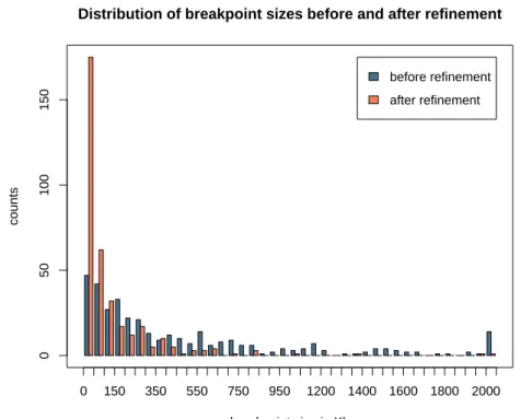
Out of the 355 refined breakpoints, only one is not significant for the permutation test of the segmentation. After further investigation, it appeared that this breakpoint corre-sponds to a mouse duplication, with the entire sequence Sr aligned with both sequences
SoAand SoB. Figure 4 shows a histogram with the sizes of the breakpoints before and after
refinement. On average, a breakpoint is reduced by 552 Kilobases and we obtained after refinement 171 (48%) breakpoints less than 50 Kb in size.
Concerning now the human-dog comparison, starting from 12839 non-overlapping one-to-one pairs of orthologous genes, we obtained 12663 within a 2−block. This led to 272 blocks and 249 breakpoints, with 240 without a human centromer in it. Table 2 gives some statitics on the blocks.
0
50
100
150
Distribution of breakpoint sizes before and after refinement
breakpoint size in Kb
counts
0 150 350 550 750 950 1200 1400 1600 1800 2000 before refinement after refinement
Figure 4: Size distribution of the 355 breakpoints between human and mouse, before and after refinement. The last box at 2 000 Kb represents values bigger than 2 Mb.
length (in bp) min max median mean
number of orthologous genes inside a 2−block 2 443 20 46.5
size of the 2−blocks before refinement (in bp) 8,382 154,604,141 3,212,701 9,945,063 size of the breakpoints before refinement (in bp) 5,963 3,108,685 241,505 437,558 size of the breakpoints after refinement (in bp) 66 1,224,273 33,140 86,074 Table 2: Description of the 2−blocks obtained between human and dog (before refinement).
The permutation test of the segmentation was significant for all the 240 refined break-points. On average, a breakpoint is reduced by 506 Kilobases, and we obtained after refine-ment 145 (60%) breakpoints less than 50 Kb in size.
3.2
Comparison with alignment-based methods
We compared the breakpoint sizes obtained by our method with those of other publicly available datasets of breakpoints. We used three datasets of breakpoints between human and mouse, all of them based on whole genome alignment methods. The first two are obtained with the algorithm GRIMM-synteny, the first one is a pairwise comparison of human and mouse [26] while the second is a multiple comparison between human, mouse and rat [7]. We call them, respectively, grimm2 and grimm3. The third one is retrieved from the Ensembl genome browser, version 34 and we call it ensembl. The method used in this case is succinctly described on the Ensembl web page2: it consists, starting with
Blastz whole genome alignments retrieved from the UCSC genome browser [21], in chaining alignments that are distant by no more than a certain max gap in number of bp, and in discarding chained blocks which span less than min len in size. It is similar to GRIMM-synteny, and to our synteny block generation method, except that conflicts are not taken into account. The breakpoints we have defined with our own method are referred to as the refinedbreakpoints, or refined for short.
For the three datasets, we computed the breakpoints as the regions between two consec-utive synteny blocks on the human genome that are not consecconsec-utive on the mouse genome. We eliminated breakpoints containing a human centromere, and when synteny blocks overlap on the human genome, we considered the intersection as the breakpoint.
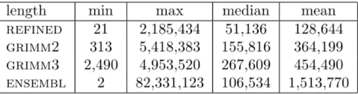
We started by globally comparing the distribution of the breakpoint sizes between the different datasets. The refined breakpoints are globally smaller than the breakpoints from the other datasets, with an average length of 129 Kb versus 364, 454 and 1513 Kb for, respectively, grimm2, grimm3 and ensembl (Table 3). We compared each dataset with ours, using the Wilcoxon rank sum test. The differences are highly significant with the respective p-values of 2.085e − 14, < 2.2e − 16 and 4.977e − 05, when compared with grimm2, grimm3 and Ensembl.
length min max median mean
refined 21 2,185,434 51,136 128,644
grimm2 313 5,418,383 155,816 364,199
grimm3 2,490 4,953,520 267,609 454,490
ensembl 2 82,331,123 106,534 1,513,770
Table 3: Comparison of the distributions of breakpoint sizes between the four datasets. The numbers are expressed in base pairs.
Since all datasets do not contain the same number of breakpoints (the refined break-points set contains 354 breakbreak-points, whereas grimm2, grimm3 and the ensembl datasets contain 246, 306 and 200 respectively), one could argue that we do not compare the same breakpoints, and that the length difference observed is only due to dataset-specific
points. In order to test this hypothesis, we compared the length of the breakpoints which are common to both the refined and the grimm3 sets. The coordinates of the grimm3 breakpoints lie on a different assembly version of the human genome (NCBI33 assembly). Using the Ensembl identifier of the orthologous genes bordering our breakpoints (as land-marks), we could unambigously identify 186 common breakpoints. For each breakpoint, we calculated the length difference between grimm3 and the refined breakpoints. The distri-bution of the length differences is plotted in Figure 5. On average, the grimm3 breakpoints are 276 Kb bigger than the refined ones, which is significant to a paired Wilcoxon test (pvalue of < 2.2e − 16).
distribution of breakpoint sizes differences
size difference in Kb counts 0 500 1000 1500 2000 0 10 20 30 40 50
Figure 5: Distribution of the differences in breakpoint sizes pairwisely computed between grimm3 and our dataset (186 common breakpoints). A positive value means that the breakpoint size is bigger in grimm3 than in our dataset. The last box at 2 000 Kb represents values bigger than 2 Mb
Observe that the refined breakpoints are computed on a more complete human genome assembly, and some gaps in the former assemblies could have prevented the detection of some synteny blocks and led to their absence from the grimm3 dataset.
We made a similar pairwise comparison with the ensembl dataset, for which the break-points lie on the same assembly version as ours. We thus eliminated this potential assembly effect. We identified 108 common breakpoints and for each one, we calculated the length dif-ference between the ensembl and the refined breakpoints. The average length difdif-ference
remains positive, meaning that the refined breakpoints are smaller than the ensembl ones (mean difference of 143 Kb). The differences are less marked, as one third of the compared breakpoints differ by less than 1 Kb (see the distribution of the length differences in Figure 6).
distribution of breakpoint sizes differences
size difference in Kb counts 0 500 1000 1500 2000 0 10 20 30 40 50 60 70
Figure 6: Distribution of the differences in breakpoint sizes pairwisely computed between ensembl and our dataset (108 common breakpoints). A positive value means that the breakpoint size is larger in the ensembl than in our dataset. The last box at 2 000 Kb represents values bigger than 2 Mb
We should however be careful with the latter results, as the ensembl dataset appeared not reliable in general. First, it contains less breakpoints than the other datasets (only 200), although it was obtained with less stringent parameters than grimm2 (for example, the minimum size of a synteny block is 100 Kb for ensembl and 1 Mb for grimm2) which should give more breakpoints. Moreover, the distribution of their length is unusual with some breakpoints very small and some very large. In particular, the biggest breakpoints (bigger than 20 Mb) make us believe that some synteny blocks may have been missed inside. Finally, if we compute the genomic coverage of the synteny blocks, we obtain that only 76.8% (2.317 Gb) of the genome is covered by the ensembl blocks, whereas the coverage is much larger for the other datasets (89.6%, 89.5% and 86.7% for grimm2, grimm3 and the 2-blocks before refinement respectively).
3.3
Genomic features in the breakpoints
Interestingly, even after refinement, the majority of the breakpoints are still big regions and are not reduced to a point. We wanted to test whether these regions have particular characteristics with respect to those inside the sequences newly appended to the synteny blocks by the refinement method. We thus compared the sequences of the breakpoints bigger than 10 Kb detected in the human-mouse comparison with their flanking sequences, defined as the regions outside the refined breakpoints which are not in the original synteny blocks (see Figure 7). We measured the coverage of each sequence in whole genome local alignments, human segmental duplications and transposable elements.
Figure 7: Schematic representation of a breakpoint. The original breakpoint (before refine-ment) lies between synteny blocks Arand Bron genome Gr, its sequence is called Sr. The
breakpoint sequence after refinement, is represented in red. The flanking sequences (showed in green) are defined as the sequences of sequence Sr that are not part of the breakpoint
region. We consider in this analysis breakpoints whose sequence (in red) spans more than 10 Kb, and for which at least one flanking sequence spans more than 10 Kb.
The motivation for measuring the presence (and amount) of whole genome (human-mouse) local alignments in a human sequence is that this is indicative of the similarity between the latter sequence and any part of the mouse genome. The whole genome local alignments were taken from the chain-net alignments files available on the UCSC genome browser [21]. The method is described in [20]. It appeared that breakpoints are depleted in local alignments (average coverage of 14%) with respect to their flanking sequences (28%) and the overall coverage of the genome (36%) (see the average distributions in Figure 8). This is statistically significant using a paired Wilcoxon test (pvalue of 2.2e − 16). Notably, 42% of the breakpoint sequences (114 breakpoints) have less than 5% of their length covered by a local alignment. Observe that these alignments are obtained from whole genome comparisons and are not necessarily part of a synteny block. It suggests that a number of breakpoints, spanning sometimes several hundreds of kilobases, do not show any similarity with any part of the other genome. Either they are very fast evolving sequences, or they correspond to insertions of new sequences in the human genome or to deletions in the mouse one.
While some breakpoints show no similarity with any part of the genome, others show similarity with several parts, either in the human or in the mouse genomes, sometimes preventing us from being able to refine them. This is the case, for instance, of segmental duplications.
0 20 40 60 80 100
Coverage in local alignments
proportion of the sequence covered by local alignments
counts
0 0.1 0.2 0.3 0.4 0.5 0.6 0.7 0.8
breakpoint sequences flanking sequences
Figure 8: Comparison of the distributions of sequence coverage by local alignments. Break-point sequences are represented in blue, whereas the flanking sequences are in orange.
Segmental duplications, also called Low Copy Repeats, are large duplications (typically greater than 1 Kb), with a high percentage of identity (typically more than 90%), that are found in a small number of copies (as opposed to transposable elements) and often clustered in mammalian genomes. Recently [2, 4, 23], it has been shown that breakpoints and duplications tend to co-localise. Two different hypotheses have been suggested to ex-plain this trend: either the duplications caused the rearrangements by similarity-dependent mechanisms, such as non allelic homologous recombination (NAHR); or the duplications accumulated at the same places because of an inherent fragility of these genomic regions. We observed here a similar trend. Breakpoints are overall more covered by segmental dupli-cations (average coverage of 27%) than their flanking sequences (average coverage of 15%). This is again statistically significant using a paired Wilcoxon test (pvalue of 2.22e − 9). Notably, 34 breakpoint sequences are almost entirely covered by segmental duplications (coverage greater than 90%).
Other duplicated sequences, that do not have necessarily the same properties as seg-mental duplications (in terms of length or similarity level) have been found associated with rearrangements. The duplicated sequences were found at each extremity of an inverted segment, in the opposite orientation [10, 19, 28]. An alternative mechanism to NAHR was suggested, which is that the duplication may have appeared as a consequence of the re-arrangement, as a fill-in of the gaps resulting from staggered break ends. Thanks to our refinement step, we can suggest candidates for this situation: this is the case when the human breakpoint sequence coincides with the mouse duplicates located in the two cor-responding breakpoints on the mouse genome, namely in sequences SoA and SoB (Figure
1). Indeed, when a breakpoint aligns with both sequence SoA and sequence SoB, it
corre-sponds to the middle segment of the numerical sequence I which contains many zeros. We can thus easily detect these special cases. For the human-mouse comparison, we obtain 41 breakpoints which present such characteristic (more than half of the middle segments of the numerical sequence I correspond to a zero, meaning these positions are covered by hits from both sequence SoA and SoB). In 36 cases, the breakpoints are absent from the human-dog
comparison, suggesting that the involved rearrangements occurred in the mouse lineage, and further arguing for a relation between duplication and rearrangement events.
Finally, we observe a similar trend for transposable elements as for whole genome local alignments and segmental duplications. Overall, breakpoints are richer in transposable elements than their flanking sequences (average coverage of 53% against 48% respectively), paired Student test significant (pvalue of 6.15e − 8). When we distinguish for the different types of transposable elements (SINEs, LINEs, LTR elements and DNA transposons), no significant difference is observed, except for LTR elements (average coverage of 11.4% in breakpoints versus 8.6% in the flanking sequences, pvalue of 2.21e − 5 for a paired Wilcoxon test).
4
Discussion
With the availability of whole genome sequences, one would have hoped to be able to com-pare genomes at the nucleotide level and thus to locate evolutionary events, such as rear-rangements, up to a base pair. Such precision is required, for instance, in order to identify potential footprints left on the sequence by a rearrangement. However, current available breakpoint data lack such precision. The goal of the method we presented in this paper is to obtain breakpoints as precise as possible. Our strategy to achieve this is divided in two steps: the first one identifies reliable blocks and the second refines the breakpoint re-gions in between using the information (corresponding to the orthologous sequences to align) obtained in the previous step.
Having reliable synteny blocks is a requirement to the refinement method, and is the reason why we chose to deal with markers that are genes. Since they are functional elements, they are usually more conserved (and so more reliable) than intergenic DNA. Moreover, orthology assignments for genes are computed at the aminoacid level, which is even more conserved. The genomic coverage of orthologous genes is less extensive than the coverage of
the alignments obtained by a whole genome comparison method which may detect similarity even in the non coding parts of the genome. It thus leads to synteny blocks which present also a low genomic coverage. However, the synteny blocks can be extended beyond the genes, and eventually we may reach a better coverage than with whole genome alignments. Nevertheless, we wish to emphasise that the method described here is not restricted to this kind of synteny blocks, and that it can also be applied on synteny blocks originally obtained from whole genome alignments for instance.
The advantage of proceeding in two steps is that by reducing the search space for homol-ogy in the first step, we can look for weaker similarity inside the breakpoint regions in the second step. This is one of the reasons why our method gives more precise breakpoints than whole genome alignment methods. Indeed, the latter operate in a single step, and require the use of stringent enough parameters to avoid obtaining blocks which are not orthologous. However, one drawback is then that they miss weak similarity inside the breakpoints.
The second argument accounting for the gain in precision of our method is based on the number of genomes compared. With the availability of an increasing number of fully sequenced genomes, methods using more than two genomes to identify synteny blocks are often privileged. However, we chose to develop a pairwise method. The motivation is to gain even further precision. Comparison of the breakpoint sizes show that 3-way blocks (such as obtained by grimm3) give bigger breakpoints than those obtained with a pairwise comparison (such as in grimm2) using the same method, even when adopting less stringent parameters. This comes from the fact that the grimm3 anchors are three-way, meaning that one anchor represents an orthologous marker in each of the three species. This leads to more confident anchors than pairwise ones, but it also reduces the set of anchors and thus the size of the synteny blocks.
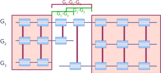
Figure 10: Example of two closely located breakpoints that appear fused when using a multiple comparison and which pairwise comparisons enable to clearly identify as two distinct breakpoints.
Although multiple comparisons could be useful to compute the synteny blocks, we argue that to refine breakpoints, a pairwise method is preferable. Indeed, this enables to be more sensitive in the detection of homology. Moreover, it also allows to discriminate between one or several rearrangement events in a seemingly common region. For example, suppose two breakpoints are very close to each other on the human genome, one being observed by comparison with the mouse genome, and the other with the dog genome. Investigating the two breakpoints by pairwise (independent) comparisons allows to determine whether they overlap position-wise as in Figure 9. Using a multiple comparison, if the two breakpoints are too close to each other (the distance between them is less than the minimum size of a synteny block), only one breakpoint may be identified. An example of this is given in Figure 10 where two distinct breakpoints are perceived as fused when doing a multiple comparison while pairwise comparisons enable to separately identify the two. It thus seems preferable to, first, identify precisely breakpoints between two genomes, and then to compare them with the breakpoints obtained in other species comparisons while trying to infer their evolutionary relationship. This strategy could be useful to estimate the amount of rearrangement re-use in independent lineages. As an example, we obtained five cases where a mouse breakpoint and a dog breakpoint do not overlap and are less than 50 Kb apart on the human genome (10 cases when the threshold is set to 100 Kb, 39 cases for 300 Kb).
Finally, comparison of the breakpoints with their flanking sequences confirms previous studies of rearrangement breakpoints where loss of similarity, enrichment in segmental du-plications and in transposable elements were revealed [2, 4, 20, 22, 23, 35]. Moreover, it
shows that breakpoints are actually regions which can be distinguished from the remaining of the genome, and reinforces the belief that breakpoints are indeed regions, and not single points.
5
Acknowledgments
The work presented in this paper was funded in part by the ACI Nouvelles Interfaces des Mathematiques (project π-vert) of the French Ministry of Research, by the ARC (projects IBN and ChromoNet) from the INRIA and by the ANR (project REGLIS No NT05-3 45205 REGLIS).
References
[1] D G Albertson, C Collins, F McCormick, and J W Gray. Chromosome aberrations in solid tumors. Nat Genet, 34(4):369–376, Aug 2003.
[2] L Armengol, M Angel Pujana, J Cheung, S W Scherer, and X Estivill. Enrichment of segmental duplications in regions of breaks of synteny between the human and mouse genomes suggest their involvement in evolutionary rearrangements. Hum Mol Genet, 12(17):2201–2208, Sep 2003.
[3] I Auger and C Lawrence. Algorithms for the optimal identification of segments neigh-borhoods. Bull. Math. Biol., 51:39–54, 1989.
[4] J A Bailey, R Baertsch, W J Kent, D Haussler, and E E Eichler. Hotspots of mammalian chromosomal evolution. Genome Biol, 5(4):R23, 2004.
[5] R Bellman and S Dreyfus. Applied dynamic programming. Princeton University Press, 1962.
[6] A Bhutkar, S Russo, T F Smith, and W M Gelbart. Techniques for multi-genome synteny analysis to overcome assembly limitations. Genome Inform, 17(2):152–161, 2006.
[7] G Bourque, P A Pevzner, and G Tesler. Reconstructing the genomic architecture of ancestral mammals: lessons from human, mouse, and rat genomes. Genome Res, 14(4):507–516, Apr 2004.
[8] G Bourque, E M Zdobnov, P Bork, P A Pevzner, and G Tesler. Comparative archi-tectures of mammalian and chicken genomes reveal highly variable rates of genomic rearrangements across different lineages. Genome Res, 15(1):98–110, Jan 2005. [9] P P Calabrese, S Chakravarty, and T J Vision. Fast identification and statistical
evaluation of segmental homologies in comparative maps. Bioinformatics, 19:i74–i80, 2003.
[10] F Casals and A Navarro. Chromosomal evolution: inversions: the chicken or the egg? Heredity, 99(5):479–480, Nov 2007.
[11] V Choi, C Zheng, Q Zhu, and D Sankoff. Algorithms for the extraction of synteny blocks from comparative maps. In WABI, LCNS, volume 4645, pages 277–288. Springer Berlin / Heidelberg, 2007.
[12] A C E Darling, B Mau, F R Blattner, and N T Perna. Mauve: multiple alignment of conserved genomic sequence with rearrangements. Genome Res, 14(7):1394–1403, Jul 2004.
[13] R W DeBry and M F Seldin. Human/mouse homology relationships. Genomics, 33:337– 351, 1996.
[14] E E Eichler and D Sankoff. Structural dynamics of eukaryotic chromosome evolution. Science, 301(5634):793–797, Aug 2003.
[15] B J Haas, A L Delcher, J R Wortman, and S L Salzberg. DAGchainer: a tool for mining segmental genome duplications and synteny. Bioinformatics, 20(18):3643–3646, Dec 2004.
[16] S Hampson, A McLysaght, B Gaut, and P Baldi. LineUp: statistical detection of chromosomal homology with application to plant comparative genomics. Genome Res, 13(5):999–1010, May 2003.
[17] H Hinsch and S Hannenhalli. Recurring genomic breaks in independent lineages support genomic fragility. BMC Evol Biol, 6:90, 2006.
[18] T J P Hubbard, B L Aken, K Beal, B Ballester, M Caccamo, Y Chen, L Clarke, G Coates, F Cunningham, T Cutts, and et al. Ensembl 2007. Nucleic Acids Res, 35(Database issue):D610–D617, Jan 2007.
[19] H Kehrer-Sawatzki, C A Sandig, V Goidts, and H Hameister. Breakpoint analysis of the pericentric inversion between chimpanzee chromosome 10 and the homologous chromosome 12 in humans. Cytogenet Genome Res, 108(1-3):91–97, 2005.
[20] W J Kent, R Baertsch, A Hinrichs, W Miller, and D Haussler. Evolution’s cauldron: duplication, deletion, and rearrangement in the mouse and human genomes. Proc Natl Acad Sci U S A, 100(20):11484–11489, Sep 2003.
[21] R M Kuhn, D Karolchik, A S Zweig, H Trumbower, D J Thomas, A Thakkapallayil, C W Sugnet, M Stanke, K E Smith, A Siepel, and et al. The UCSC genome browser database: update 2007. Nucleic Acids Res, 35(Database issue):D668–D673, Jan 2007. [22] J Ma, L Zhang, B B Suh, B J Raney, R C Burhans, W J Kent, M Blanchette, D Haussler,
and W Miller. Reconstructing contiguous regions of an ancestral genome. Genome Res, 16:1557–1565, Sep 2006.
[23] W J Murphy, D M Larkin, A Everts van der Wind, G Bourque, G Tesler, L Auvil, J E Beever, B P Chowdhary, F Galibert, L Gatzke, and et al. Dynamics of mam-malian chromosome evolution inferred from multispecies comparative maps. Science, 309(5734):613–617, Jul 2005.
[24] J H Nadeau and B A Taylor. Lengths of chromosomal segments conserved since diver-gence of man and mouse. Proc Natl Acad Sci U S A, 81(3):814–818, Feb 1984.
[25] X Pan, L Stein, and V Brendel. SynBrowse: a synteny browser for comparative sequence analysis. Bioinformatics, 21(17):3461–3468, Sep 2005.
[26] P Pevzner and G Tesler. Genome rearrangements in mammalian evolution: lessons from human and mouse genomes. Genome Res, 13(1):37–45, Jan 2003.
[27] P Pevzner and G Tesler. Human and mouse genomic sequences reveal extensive break-point reuse in mammalian evolution. Proceedings of the National Academy of Sciences U.S.A., 13:7672–7677, 2003.
[28] J M Ranz, D Maurin, Y S Chan, M von Grotthuss, L W Hillier, J Roote, M Ashburner, and C M Bergman. Principles of Genome Evolution in the Drosophila melanogaster Species Group. PLoS Biol, 5(6):e152, Jun 2007.
[29] L Rieseberg. Chromosomal rearrangements and speciation. Trends Ecol Evol, 16(7):351–358, Jul 2001.
[30] A Ruiz-Herrera, F Garc`ia, E Giulotto, C Attolini, J Egozcue, M Pons´a, and M Gar-cia. Evolutionary breakpoints are co-localized with fragile sites and intrachromosomal telomeric sequences in primates. Cytogenet Genome Res, 108(1-3):234–247, 2005. [31] S Schwartz, W J Kent, A Smit, Z Zhang, R Baertsch, R C Hardison, D Haussler, and
W Miller. Human-mouse alignments with BLASTZ. Genome Res, 13(1):103–107, Jan 2003.
[32] A U Sinha and J Meller. Cinteny: flexible analysis and visualization of synteny and genome rearrangements in multiple organisms. BMC Bioinformatics, 8:82, 2007. [33] P Stankiewicz and J R Lupski. Genome architecture, rearrangements and genomic
disorders. Trends Genet, 18(2):74–82, Feb 2002.
[34] F Swidan, E P C Rocha, M Shmoish, and R Y Pinter. An integrative method for accurate comparative genome mapping. PLoS Comput Biol, 2:e75, 2006.
[35] P Trinh, A McLysaght, and D Sankoff. Genomic features in the breakpoint regions between syntenic blocks. Bioinformatics, 20 Suppl 1:I318–I325, Aug 2004.
Unité de recherche INRIA Futurs : Parc Club Orsay Université - ZAC des Vignes 4, rue Jacques Monod - 91893 ORSAY Cedex (France)
Unité de recherche INRIA Lorraine : LORIA, Technopôle de Nancy-Brabois - Campus scientifique 615, rue du Jardin Botanique - BP 101 - 54602 Villers-lès-Nancy Cedex (France)
Unité de recherche INRIA Rennes : IRISA, Campus universitaire de Beaulieu - 35042 Rennes Cedex (France) Unité de recherche INRIA Rocquencourt : Domaine de Voluceau - Rocquencourt - BP 105 - 78153 Le Chesnay Cedex (France)