Analysis of complex viscoelastic flows using a finite element method

(1)

Analysis of Complex Viscoelastic Flows Using a

Finite Element Method

bv

Scott David Phillips

TP q ,/I (,,.'- (1 QiJO fI-

MASSACHUSETT

OF TECHN(

FEB 2 5

LIBRAF

1/I

Su11)l1ut

t,('d to te Department of Chemnlical

Engineering

in partial flfillment of the requirenments for the egree of

Doc:tor of Philosophy

at the

NI ASSAC 1H SETTiS 1 NSTITUTI E OF TECH NOLOGY

February 2006

®

NhMassachlset

l.s Institute of Technology 2006

Signat

ure

of

Autho1

... .... . .. ...

Department of

Cerrtifiecd i)...

Chemic:al Engineering

Febritary 1st. 2006 .

Professor of

Robert A. Brown

(]henieal Engineering

T

hesis Supervisor

(Cc'frtifi cd b ...

Professor of

iAc.epte.( b ...

Robert C. Arnst rong

Chemical Engineering

Thesis Spplervisor

... .. ...

William N*. Deen

II

S INSTITUTE 2006 *IES -1-1 . ki . . I t 11 A I'Vc, VI 11.1 V IQ-,-L DI U --j '

ItLAPi

(2)

Analysis of Complex Viscoelastic Flows Using a Finite Element

Method

by

Scott David Phillips

Submitted to the Department of Chemical Engineering

on February 1st, 2006, in partial fulfillment of the requirements for the degree of

Doctor of Philosophy

Abstract

The field of computational fluid mechanics of viscoelastic flows has been well explored in the three decades since its inception. Still, even with the vast amount of work detailed in the literature, much remains to be done towards the improvement of models of viscoelastic fluids and the improvement of the numerical methods used to solve the set of governing equations. The work contained in this document is concentrated in the latter of these areas.

The main goal of this body of work is to develop a robust, efficient simulation package to model three-dimensional viscoelastic flows. In order to accomplish this goal, improve-ments to the numerical methods and equation formulation were necessary to help reduce the overall size of the equation set used to describe viscoelastic flows in three-dimensional geometries. In order to test their viability for use in reducing the overall size of the prob-lem, concepts involving changing the formulation of the equations and the numerical methods used to find the solution to the equations were first implemented and analyzed in a previously developed two-dimensional finite element simulation package.

Implementation and analysis is discussed of a formulation change involving decoupling the calculation of the velocity gradient interpolant equation and the momentum and mass continuity equations in the DEVSS-G formulation. Two different decoupled methods for computing the velocity gradient, one using a global least squares approximation and the other a local patch algorithm, are explored. While both methods reduce to the true velocity gradient with mesh refinement, the patch algorithm is shown to require significantly more mesh refinement than the global least squares approximation to order to attain equivalent refinement of the solution. Comparison of the two methods taking into account the additional refinement requirements of the local patch algorithm makes clear the superiority of the decoupled global least squares approximation for calculation of the velocity gradient interpolant.

(3)

demonstrated through the addition and modification of the evolution equations describing the stress of the polymer as well as new physical quantities of the flow. A time-dependent, free-surface finite element method is developed in which an evolution equation derived from the kinematic boundary condition is used to describe the height of the free surface as a function of time. This new evolution equation is incorporated into the decoupled formulation by simply adding an additional step to the time integration to evaluate the change in the height of the surface during the current timestep and then updating the element locations in the deformable region of the mesh. Application of the new equation in this manner requires no knowledge of the direct dependence of the system on changes in the new quantity, allowing for quick and easy implementation.

Incorporation of more advanced constitutive equations is used as further example of the utility of the decoupled form of the DEVSS-G equations. For most continuum based constitutive equations, the dependence of the equations on the flow variables can be expressed explicitly, allowing for the coupled set of equations to be solved with Newton's method. However, the dependence of the stress on the flow cannot be explicitly written for more advanced constitutive equations such as those derived from kinetic theory or those employing Brownian dynamics, greatly hindering the performance of Newton's method in locating the solution to the system. As an illustrative example, incorporation into the decoupled equation formulation of the closed form of the Adaptive-Length-Scale model (ALS-C) is presented. Simulations are presented capturing for the first time the pressure drop enhancement with increasing viscoelasticity of the model of the flow of a Boger fluid in the 4:1:4 axisymmetric contraction-expansion geometry observed experimentally (Rothstein et al., 2001). Simulations of the flow of a 4-mode FENE-P model fluid within the geometry are also presented. Though its dependence on the flow field can be expressed analytically, the cost of computation using multimode models is typically prohibitive when using fully coupled equation sets as the overall problem size grows considerably with the addition of each new mode. Incorporation of the 4-mode model within the decoupled equation formulation adds relatively little computational cost to the overall calculation.

Employing the formulation and numerical methods developed herein, a new three-dimensional finite element package is described for simulating confined viscoelastic flows. To make the package more robust, a number of different boundary conditions are in-cluded for modeling different geometries used in polymer processing. To help reduce the burden associated with mesh refinement in three-dimensional meshes, a commercial meshing package utilizing o-grid refinement for localization of refinement is employed. Furthermore, to allow for computation of the large equation sets typically associated with three-dimensional geometries, a parallel implementation of the three-dimensional simulation package is developed based on the two-dimensional parallel method devel-oped by Caola et al. ((Caola et al., 2001), (Caola et al., 2002)). Simulation results demonstrating the accuracy and performance of the method are presented.

As a test of the robustness of the three-dimensional method, simulations of the flow of Newtonian and Oldroyd-B fluids through a periodic, linear array of cylinders are

(4)

presented. Comparisons with previous calculations for the Oldroyd-B flow in an infinitely wide domain with no variations in the direction of the width show the same trend in the drag force on the cylinder with increasing viscoelasticity as well as in the size and shape of the vortices formed in the gap between the cylinders. The study of this flow includes effects of modeling the cross section of the flow as an infinite domain with no variation in the direction of the width, an infinite domain of periodic computational width, an infinite domain of periodic computational width and a symmetric flow above and below the cylinders, and a bounded domain with solid walls located 4 cylinder radii apart. Thesis Supervisor: Robert A. Brown

Title: Professor of Chemical Engineering Thesis Supervisor: Robert C. Armstrong Title: Professor of Chemical Engineering

(5)

...

(8)

8.3 Conclusions ... 248

9 Conclusions and Further Work 251

9.1 Summary of work ... 251

(9)

List of Figures

1-1 Example of the reduction in dimensionality of the modeling of the flow field in simple Couette flow from three dimensions shown in the main figure to one dimension shown in the inset. This reduction in dimesionality is

appropriate only when vo = vo (r). ... 29

1-2 View of the gap cross-section of the low viscosity Boger fluid at De = 1.88, Re = 33.4 (co-rotating cylinders). Downwardly rolling vortices begin to form at 10 minutes. The direction of rotation of vortices along the inner cylinder is reveled by the clockwise motion of the comma shaped region of seed depletion in the vortex visible from 40 to 44 minutes. Reproduced

from [9] ... 30

1-3 Steady, spatially periodic structure of a Boger fluid flowing past an isolated

cylinder (black). Flow is from top to bottom. Reproduced from [57] . 32

1-4 Example of an instability arising in the extrusion of a single strand polymer filament. Steady flow is shown in (a), evolving into a shark-skin instability in (b)-(e), and finally gross melt fracture in (f) and (g). Extrudates of a polymer melt at 70° C. Shear rates are (a) 1.36 s-l, (b) 2.72 s-_{1, (c)}

6.81 s- 1, (d) 13.6 s- 1. (e) 34.1 s-l, (f) 68.1 s- 1, and (g) 136 s- 1. Fiber is

roughly 1 mm in diameter. Reproduced from [88]. ... 33

(10)

1-6 Artist rendition of a 4 DG Deep-Groove fiber. The cross-section is de-signed to have enhanced capillary action allowing for improved wicking properties as well as greatly increased surface to volume ratio over

tradi-tional fibers. Reproduced from [2] ... .. 34

1-7 Possible die geometry and cross-section with five hole layout ... 34

2-1 Tube flow and "shear thinning." In each part, the Newtonian behavior is shown on the left "N"; the behavior of a polymer on the right "P". (a) A tiny sphere falls at the save rate through each; (b) the polymer flows out

faster than the Newtonian fluid. Reproduced from [10] ... 42

2-2 Fixed Cylinder with rotating rod. "N" The Newtonian liquid, glycerin, shows a vortex; "P" the polymer solution, polyacrylamide in glycerin, climbs the rod. The rod is rotated much faster in the glycerin than in the polyacrylamide solution. At comparable low rates of rotation of the shaft, the polymer will climb whereas the free surface of the Newtonian

liquid will remain flat. Reproduced from [10] ... 44

2-3 Die swell for liquid extruded into a neutrally-bouyant medium constructed from a low viscosity silicone oil and carbon tetrachloride solution of match-ing density to the extruded flow medium. (a) Newtonian liquid of viscosity 11.6 Pa s being extruded (Re=0.001). (b) Boger fluid of viscosity 11.4 Pa

s being extruded (Re=0.0009, We=0.272). Reproduced from [12] ... . 46

2-4 Steady simple shear flow with shear rate r = V/b. Reproduced from [10]. 48

2-5 Deformation of (a) unit cube of material from time t to t2 (t2 > t1) in (b) steady simple shear flow and (c) three kinds of shearfree flow. The volume of material is preserved in all of these flows. Reproduced from [10] 49 2-6 Steady elongational flow (shearfree flow with b = 0 and e > 0).

(11)

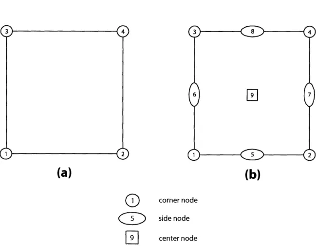
3-1 Line elements used to discretize one-dimensional geometries. (a): 2-node

linear line element; (b): 3-node quadratic line element. ... 66

3-2 Quadrilateral elements used to discretize the surfaces of a three-dimensional geometry. (a): 4-node bilinear quadrilateral element; (b): 9-node

bi-quadratic quadrilateral element ... 68

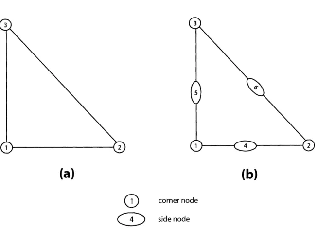
3-3 Triangle elements used to discretize the surfaces of a three-dimensional geometry. (a): 3-node bilinear triangle element; (b): 6-node biquadratic

triangle element. ... 70

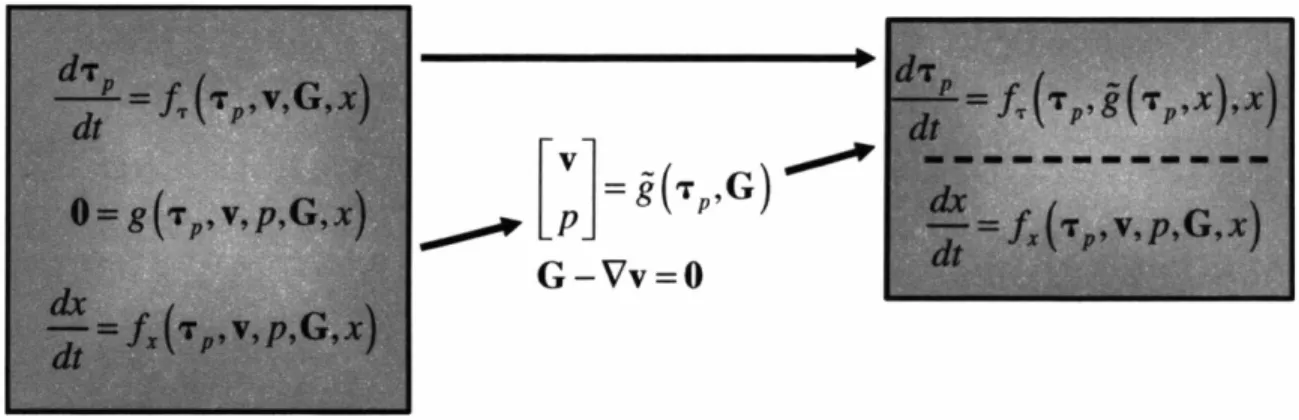
3-4 Illustration of the index one set of differential algebraic equations for the viscoelastic flow problems. The set of DAE's can be rewritten as a set of

ODE's describing the stress evolution which are constrained by the flow

equations ... 73

3-5 Speedup S for the solution of the Stokes-like linear system; De=0.5. The meshes range in size from mesh SM1 with 60,900 degrees of freedom to

mesh SM4 with 751,110 degrees of freedom. Figure reproduced from [16] 80

3-6 Finite element mesh used in simulation of the melt spinning process. The

mesh contains 3896 elements and 92418 unknowns. Note that this

un-konwn count is for continuous linear stress unkowns. Taken from [44]. 81

4-1 Time stepping algorithm of the decoupled G formulation for the equations

describing viscoelastic flow. ... 87

4-2 Four quadralateral elements used in construction of the local patch. The resulting patch element is an approximation of a larger quadralateral

ele-ment

.. ... . ... 89

4-3 Types of patch element configurations for a mesh of quadralateral ele-ments. Each of the three cases has four possible orientations relative to

(12)

4-4 Schematic diagram of a wavy walled channel. H = 0.8 is the channel

height at the widest point; H, = 0.2 is the amplitude of the sine wave describing the undulations in the top wall; Lp = 1.0 is the length of a

periodic section of the channel. ... 92

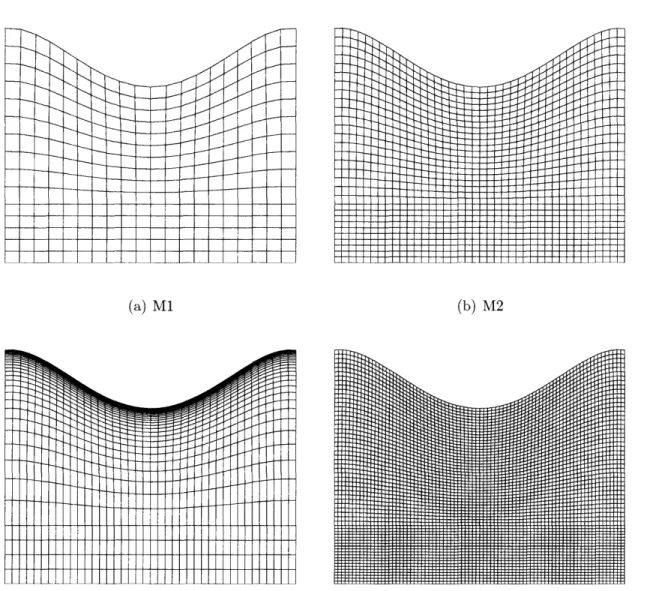
4-5 Meshes for the wavy-walled channel geometry. M: 300 elements; M2:

1200 elements, M2a: 1150 elements; M3: 4800 elements ... 94

4-6 Error associated with decoupling of the global minimization equations for the velocity gradient interpolants from the momentum and mass continuity equations in startup of flow in the wavy-walled channel of an Oldroyd-B

fluid of B = 0.5 and De = 0.7. -: A IIVII;- -:

IHrfll

. 95

4-7 Convergence of the flow in the wavy-walled channel using the decoupled global minimization method for computation of the velocity gradient in-terpolant with a fixed stress field. Stress field computed using the fully coupled method for the flow of an Oldroyd-B fluid of 3 = 0.5 with De = 0.7. 97 4-8 Velocity and pressure contours computed with the global and local

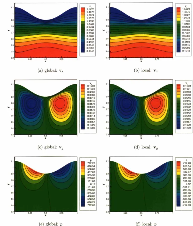
smooth-ing methods with mesh M2a for De = 0.1. ... 98

4-9 Comparison of the velocity and pressure contours computed with the global and local smoothing methods with mesh M2a for De = 0.1. Blue:

global method; red: local method ... 99

4-10 Velocity and pressure contours computed with the global and local

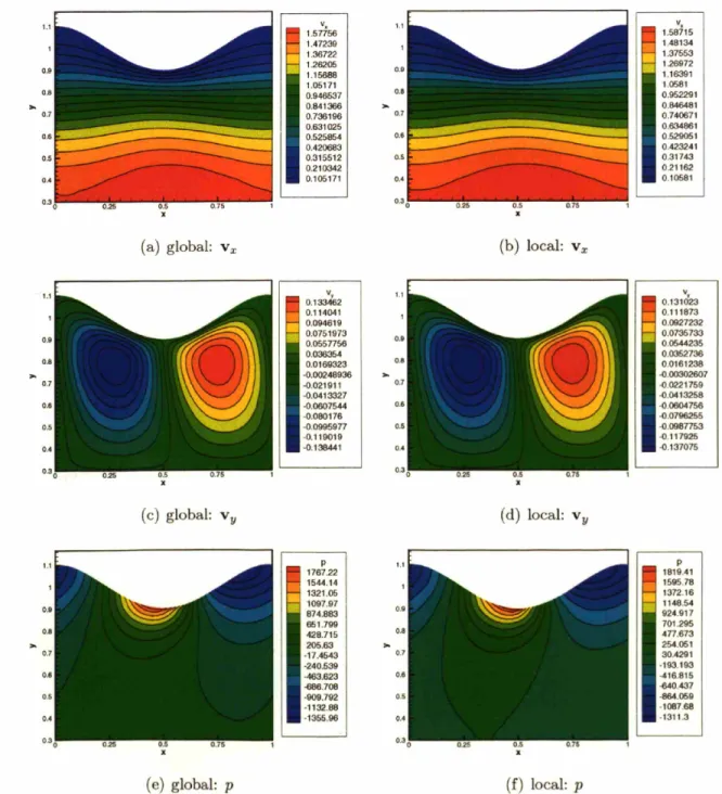
smooth-ing methods with mesh M2a for De = 1.0. ... 101

4-11 Comparison of the velocity and pressure contours computed with the global and local smoothing methods with mesh M2a for De = 1. Blue:

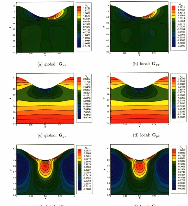
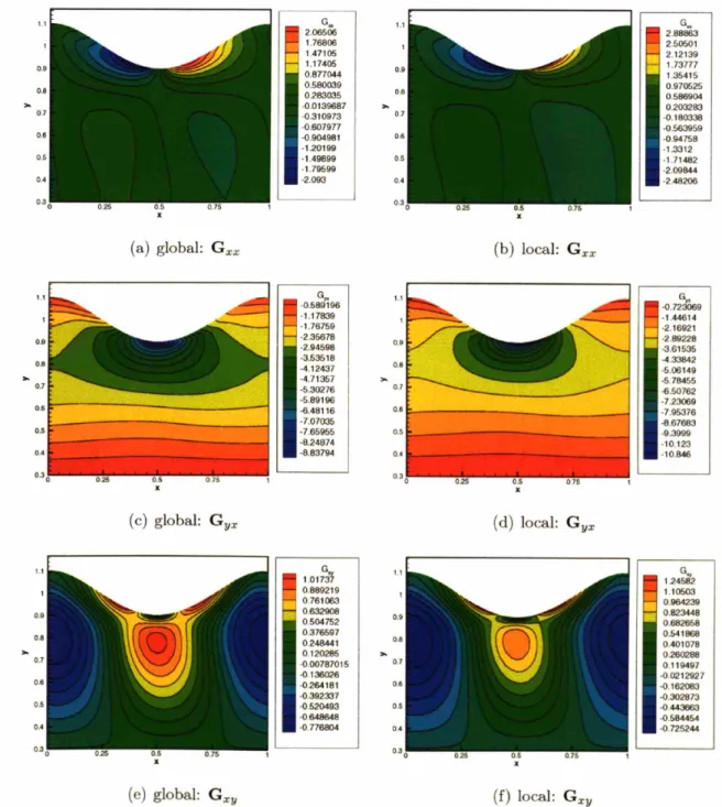
4-12 Contour plots of the components of G computed using the global and local

(13)

4-13 Comparison of the contours of the components of G computed with the global and local smoothing methods with mesh M2a for De = 0.1. Blue:

4-14 Contour plots of the components of G computed using the global and local

minimization methods with mesh M2a for De=1.0. ... 106

4-15 Comparison of the contours of the components of G computed with the global and local smoothing methods with mesh M2a for De = 1.0. Blue:

4-16 Convergence of the L2norm of the velocity field in the wavy-walled channel

using the decoupled local smoothing method (- -) for computation of

the velocity gradient interpolant with a fixed stress field. Stress field computed using the fully coupled method for the flow of an Oldroyd-B fluid of 3 = 0.5 with De = 0.7. Decoupled global minimization method

(-) is included for comparison. ... 108

4-17 Difference in L2 norms of the velocity computed from the global and local

smoothing methods using a fixed stress field over a range of De for an Oldroyd-B fluid with = 0.5. Mesh M2a is used in the calculations. . . 109

4-18 Mesh convergence study of the local smoothing method. Refinement r

is inversely proportional to the element dimensions in the mesh. (--): global method with mesh M1; (o): local method. G,X on channel wall at

x =: 0.65 .. 1... 110

4-19 Refinement necessary when using local smoothing method to converge to

global smoothing method solution. Shaded regions highlight areas of

refinement. The darker shaded region requires 4 times refinement in both the x and y directions. The lighter shaded region requires 4 times refinement in x and 2 times in y. The unshaded region requires no refinement. 112

(14)

5-1 Schematic diagram of the change in the height of the surface after time At as described by the y component of the normal velocity of the fluid.

(-): surface at t = to; (- -): surface at t = to + At. ... 120

5-2 Schematic diagram of the change in the height of the surface after time At as described by equation 5.6. (-): surface at t = to; (- -): surface

at t = to + At; (- -): surface at t = to + At accounting for translation. 121

5-3 Decoupling of equation set describing the time-dependent viscoelastic flow

problem with free-surface boundaries ... 124

5-4 Subset steps in a single timestep for the free-surface time integrator. Ar-rows indicate both progression of algorithm as well as flow of information

between subproblems . . . .... 125 5-5 Successive levels of mesh refinement in region surrounding the die lip. Die

lip located at x = 0, y = 1 ... 126

5-6 Die-swell ratio versus level of mesh refinement around die lip for flow of a Giesekus fluid ( = 0.2, = 0.5) through a contraction die-swell geometry. 128 5-7 Planar die-swell geometry. H: upstream height; h: contractoin height; L:

contraction length; hf: maximum swell height. ... 129

5-8 Contraction die-swell mesh used for comparisons of the time-dependent

and steady-state free-surface solvers. ... 129

5-9 Contour plots of pressure and velocity for flow through the contraction die-swell geometry with We = 1, L/h = 2.5, and Ca = 1 for the Giesekus model ( = 0.2 and / = 0.5) as computed with the time-dependent method. 130 5-10 Die-swell ratio versus Weisenberg number for flow of a Giesekus model

(a = 0.2 and /3 = 0.5) in a contraction die-swell geometry with L/h = 2.5

and Ca = 1. (--): steady-state method; (A): time-dependent method. 132

5-11 Die-swell ratio versus die land length for flow of a Giesekus model (a = 0.2 and 3 = 0.5) in a contraction die-swell geometry with Wi = 4 and Ca = 1.

(15)

5-12 Die-swell ratio versus capillary number for flow of a Giesekus model (a = 0.2 and = 0.5) in a contraction die-swell geometry with We = 4 and

L/h = 2.5. (--): steady-state method; (A): time-dependent method. . 134

6-1 4:1:4 contraction expansion geometry selected to model the experimental geometry of Rothstein et al. [65]. Flow through the geometry is from top to bottom. Here R1 = 4R2, L = R2, Lu = 24R2, Ld = 25R2, RC = 0.5R2,

and R 2 = 0.2R 2. . . . . . . . . ... 138

6-2 Finite element mesh necessary to discretize 4:1:4 contraction-expansion

geometry ... 144

6-3 Level of refinement necessary near the contraction wall to resolve areas of high gradients. . . . ... .. .... 145 6-4 Fit of single mode plus solvent to the dynamic viscosity data obtained

from experiments. (0): 0.025% PS/PS fluid; (--): model. .... . 148

6-5 Fit of single mode plus solvent to the experimental dynamic rigidity data.

From experiments: (0): 0.025% PS/PS fluid. From model: (--):

polymer mode; (- .): solvent mode; ( ): model composite ... 149

6-6 Fit of 4 mode plus solvent to the experimental dynamic viscosity data.

(0): 0.025% PS/PS fluid; (-- ): model. ... 150

6-7 Fit of 4 mode FENE-P plus solvent model to the experimental dynamic

rigidity data. From experiments: (0): 0.025% PS/PS fluid. From

model: (- -): mode 1; (- .): mode 2; (): mode 3; (-- -): mode 4;

(--· ): solvent mode; (-): model composite ... 151

6-8 Transient extensional viscosity of the single mode models with b = 7744.

(0): 0.025% PS/PS fluid; (-): FENE-P; ALS-C model with (-- -):

z = 0.25; ) z=0.5; (-): z = 1.0; ( .): z= 2.0 ... 152

6-9 First normal stress coefficient for the single mode models with b = 7744. (O): 0.025% PS/PS fluid; (-): FENE-P; (- -): z = 0.25; (-- ): z = 0.5;

(16)

6-10 Transient extensional viscosity of the 4 mode FENE-P model. (0):

0.025% PS/PS fluid; (-- -): 4 mode FENE-P; (-): 1 mode FENE-P;

(- ): ALS-C with z = 0.5 ... 155

6-11 First normal stress coefficient for the 4 mode FENE-P model. (0):

0.025% PS/PS fluid; (-- ): 4 mode FENE-P; (-): 1 mode FENE-P;

( ): ALS-C with z = 0.5 ... 156

6-12 Contours of pressure for flow in the 4:1:4 geometry for the ALS-C model

with z = 0.25. (a): De = 0.5; (b): De = 3.0; (c): De = 6.0; (d):

De = 9.0; (e): De = 12.0; (f): De = 16.0. ... 157

6-13 Contours of pressure for flow in the 4:1:4 geometry for the ALS-C model

De = 9.0; (e): De = 12.0; (f): De = 16.0. ... 158

6-14 Contours of (bseg) for flow in the 4:1:4 geometry for the ALS-C model with z =- 0.25. (a): De = 0.5; (b): De = 3.0; (c): De = 6.0; (d): De = 9.0;

(e): De = 12.0; (f): De = 16.0 ... 159

6-15 Contours of (bseg) for flow in the 4:1:4 geometry for the ALS-C model with z = 1.0. (a): De = 0.5; (b): De = 3.0; (c): De = 6.0; (d): De= 9.0;

(e): De = 12.0; (f): De = 16.0 ... 160

6-16 Contours of tr (QQ) for flow in the 4:1:4 geometry for the ALS-C model

De = 9.0; (e): De = 12.0; (f): De = 16.0. ... 161

6-17 Contours of tr (QQ) for flow in the 4:1:4 geometry for the ALS-C model with z = 1.0. (a): De = 0.5; (b): De = 3.0; (c): De = 6.0; (d):

De = 9.0; (e): De = 12.0; (f): De = 16.0. ... 162

6-18 Extra pressure drop of the single mode fluid the 4:1:4 contraction-expansion

geometry. (0): 0.025% PS/PS fluid; ( ): FENE-P; (--): z = 0.25;

(-- ): z = 0.5; (): z = 1.0; ( . .): z =2.0 ... 165

(17)

6-20 Key measurements for characteristics of upstream corner vortex. Z and R, are the axial and radial distance, respectively, of the vortex center from the salient corner upstream of the contraction. L is the vortex

reattachment length ... 166

6-21 Streamlines near the salient corner of the 4:1:4 contraction-expansion with increasing Deborah number for the ALS-C model with z = 1.0. (a): De =

0.5; (b): De = 3.0; (c): De = 6.0; (d): De = 9.0; (e): De = 12.0; (f):

De = 16.0 ... 167

6-22 Streamlines near the salient corner of the 4:1:4 contraction-expansion with increasing Deborah number for the ALS-C model with z = 0.25. (a):

De =0.5; (b): De =3.0; (c): De = 6.0; (d): De = 9.0; (e): De =12.0;

(f): De = 16.0 ... 168

6-23 Key characteristics of the vortex formed in the upstream salient corner with increasing Deborah number for the ALS-C fluid where X = L/,IR₂ is

the vortex reattachment length, = R/R 2is the radial location of vortex

center, and C = Zv/R 2 is the upstream location of the vortex center.

(--): z=0.25; (-.): z=0.5; (): z=1.0; (- .): z=2.0 ... 170

6-24 Characteristics of the upstream growth dynamics as a function of Deborah number for the 4:1:4 axisymmetric contraction-expansion with rounded entrance lip, Rc = 0.5R2 - (): vortex reattachment length, X = Lv/R2;

(Ai: radial location of vortex center, f = Rv/R2; () the upstream

location of the vortex center, C = Zv/R2; and (): vortex reattachment

length for the 4:1:4 contraction-expansion with sharp entrance lip, R, = 0. Reproduced from [65]. Note: De scale has been modified to correspond

with the current work. ... 171

6-25 Extra pressure drop of the single and 4-mode models in the 4:1:4

contraction-expansion geometry. (0): 0.025% PS/PS fluid; ( ---): 4-mode

(18)

6-26 Key characteristics of the vortex formed in the salient corner with increas-ing Deborah number for the sincreas-ingle and 4-mode fluids. 4-mode FENE-P:

(--- ); ALS-C: (--): z=0.25; (.): z=1.0 ... 174

7-1 Hexahedral elements used to discretize the volume of a three-dimensional geometry. (a): 8-node linear hexahedral element; (b): 27-node quadratic hexahedral element. (J, r, ~) isoparametric coordinate system is shown

for each element. ... 181

7-2 Tetrahedral elements used to discretize the volume of a three-dimensional geometry. (a): 4-node linear tetrahedral element; (b): 10-node quadratic tetrahedral element. Tetrahedral (r, s, t) isoparametric coordinates are

shown for each node in the two elements ... 184

7-3 Example of o-grid refinement in a two-dimensional mesh used to localize the effects of mesh refinement. a) standard mesh with 4 elements in each section. b) mesh with o-grid refinment applied to central section, doubling the refinement. . . . 186 7-4 Schematic diagram of a pipe with circular cross-section. Flow is in the

x direction. Inflow and outflow faces are in the yz plane. L = 5 is the length of the pipe used in the simulations. D = 2 is the diameter of the pipe used in the simulations. Note that Cartesian coordinates are used

to describe the structure in three-dimensional space ... 188

7-5 Mesh used for simulations of flow of a fluid in a pipe with cylindrical

cross-section. The mesh contains 1344 hexahedral elements. ... 189

7-6 Comparison of the velocity field generated with the three-dimensional fi-nite element package to the analytical solution for flow of a Newtonian

fluid in a cylindrical pipe. - -: analytical solution; 0: finite element

solution ... 190

7-7 Mesh used for simulations of flow of a fluid in a pipe in the two-dimensional finite element method. The mesh contains 56 quadrilateral elements. .. 191

(19)

7-8 Comparison of the velocity field generated with the three-dimensional fi-nite element package and the two-dimensional fifi-nite element package used

in [16] for flow of a Giesekus model fluid in a cylindrical pipe.

Parame-ters for the model fluid are = 0.5, De = 1.0, and a = 0.1. - -: 2-D

axisymetric solution; 0: 3-D solution ... 192

7-9 Comparison of the shear and normal components of the stress tensor gen-erated with the three-dimensional finite element package and the two-dimensional finite element package used in [16] for flow of a Giesekus model fluid in a cylindrical pipe. Parameters for the model fluid are = 0.5, De = 1.0, and a = 0.1. Symbols represent the solution from the 3-D package, and lines represent the same from the 2-D package. - - and 0:

; --and

I:

; -- -and V: yx .. 193

7-10 Schematic of flow in a rectangular duct. Flow is in the x direction. Inflow and outflow faces are in the yz plane. L = 2 is the length of the duct

used in the simulations. 2H = 1 is the height of the duct and 2W = 1 is

the width of the duct. ... 194

7-11 Schematic of flow between parallel plates. Flow is in the x direction. Inflow and outflow faces are in the yz plane. L = 2 is the length of the duct used in the simulations. 2H = 1 is the height of the duct used in the simulations. . . . ... 194 7-12 Mesh used for simulations of flow of a fluid in a duct with a square

cross-section. The mesh contains 600 hexahedral elements ... 195

7-13 Comparison of the velocity field generated with the three-dimensional fi-nite element package to the analytical solution for flow of a Newtonian fluid between parallel plates. - -: analytical solution; 0: finite element

(20)

7-14 Comparison of the velocity field generated with the three-dimensional fi-nite element package to the analytical solution for flow of a Newtonian fluid in a duct with a square cross section. - -: analytical solution at z =- 1/3; [-: finite element solution at z = 1/3;-: analytical solution at

z = 1/2;

0:

finite element solution at z = 1/2. ... 198

7-15 Secondary flow generated in the flow of an MPTT fluid in a square duct. The image shows streamtraces in a single quadrant of the cross-section of the duct. Model parameters as reported in [86] are p = 1, TmO = 1,

Amax, = 0.01, = 0.1, = 0.2, n = 0.65, and = 1. Figure reproduced

from [86]. ... 199

7-16 Secondary flow generated from flow of a Giesekus fluid with /, = 0.5, De = 1.0, and a = 0.1 in a square duct of 2H = 1, 2W = 1, and L = 2. Symmetry clearly present along y = 0.5, z = 0.5, y = z, and y = 1 - z

planes ... 200

7-17 Speedup and efficiency of three-dimensional parallel method for flow of a Giesekus fluid (De = 1.0,

/

= 0.5, a = 0.1) in a square duct. The mesh

consists of 5,000 elements and a total of 450,000 unknowns ... 203

7-18 Gustafson efficiency as a function of the number of processors in the par-allel machine for the three-dimensional finite element solver. Unknowns

per processor: 0- 14115, C- 44788, A- 177088. ... 204

8-1 Schematic diagram of the periodic array of cylinders. The distance be-tween the cylinder centers is L = 2.5Rc. The height of the channel is

2H = 4R,. The axis of the cylinder is centered between the top and bot-tom walls of the channel. The width of the channel is W = 4R, for the

majority of the calculations, though geometries of W = 2R, and W = 3R, are also simulated. The periodic computational domain is from the center of gap fore and aft of one cylinder with a length of Ld = L,, denoted by the dashed lines. The flow in the channel is in the positive x direction. . 208

(21)

8-2 The mesh used for simulation of the three-dimensional bounded and peri-odic width geometries. The mesh is composed of 14420 hexahedral elements.212 8-3 The symmetric mesh used for simulation of the three-dimensional bounded

and periodic width geometries. The mesh is identical to the upper half of the three-dimensional mesh shown in Fig. 8-2 and is composed of 7210 hexahedral elements. . . . ... 213 8-4 The two-dimensional mesh used in simulations of the periodic, linear array

of cylinders where variations in the z direction have been neglected and the veloctiy in the z direction is assumed to be zero. The mesh is a cross-section of the three-dimensional mesh and consists of 412 quadrilateral

elements ... 214

8-5 Contour plots of the periodic portion of pressure and the x and y compo-nents of the velocity for the flow of a Newtonian fluid in a periodic, linear array of cylinders with infinite width. Variations in the z direction and

the z velocity are neglected. ... 216

8-6 The streamlines for the flow of a Newtonian fluid in a periodic, linear array of cylinders with infinite width. Variations in the z direction and the z

component of velocity are neglected. ... 217

8-7 Contour plots of the periodic portion of pressure and the x and y compo-nents of the velocity in the z = 0 plane for the flow of a Newtonian fluid in a periodic, linear array of cylinders with periodic width of W = 4Rc. . 218 8-8 The streamlines of the flow of a Newtonian fluid through a periodic array

of cylinders unbounded in the z direction with periodic width of W = 4.

Flow is in the positive x direction ... 219

8-9 Contour plots of the periodic portion of pressure and the x and y compo-nents of the velocity in the z = 1 plane for the flow of a Newtonian fluid

(22)

8-10 The streamlines of the flow of a Newtonian fluid through a periodic array of cylinders bounded in the z direction with width W = 4Re. (a) z = 0 plane; (b) z = R plane. Flow is in the positive x direction. ... 223 8-11 Plot of streamlines near the gap between the cylinders overlaid on a

con-tour plot of the positive and negative regions of the y component of velocity. 224 8-12 Velocity in the y direction along the line x = 1 (z = 0). The intersections

with the v, = 0 line correspond to the separation lines between the main

flow and the vortex, and the vortex/vortex interface. ... 225

8-13 Velocity in the y direction along the line x = 1 (z = 0) for the four variations in the width of the periodic, linear array of cylinders. (green): infinite width, no z variations; (orange): periodic width; (red): periodic width, forced symmetry; (blue): bounded width. . . . .... 226 8-14 Isosurface for v, = 0 near the downstream edge of the cylinder for a

Newon-tian fluid flowing in the periodic, linear array of cylinders with periodic

width of W = 4R,. The region between the downstream cylinder wall

and the yz plane at x = 1.25 is shown. The upper and lower isosurface near the cylinder wall denotes the interface between the main flow and the vortices. The center isosurface denotes the interface between the vortices.

The red line is at x = 1. ... 227

8-15 Isosurface for vy = 0 near the downstream edge of the cylinder for a Newon-tian fluid flowing in the periodic, linear array of cylinders with periodic

width of W = 4R,. The region between the downstream cylinder wall

and the yz plane at x = 1.25 is shown. The upper and lower isosurface near the cylinder wall denotes the interface between the main flow and the vortices. The center isosurface denotes the interface between the vortices.

(23)

8-16 Streamlines computed for the flow of an Oldroyd-B fluid with d = 0.67

and De of 0.0, 0.7, and 1.5 in a periodic, linear array of cylinders with infinite width where variations in the z direction are neglected and vz is

assumed to be zero ... 230

8-17 Contours of rp11 (left) and 7rp2 (right) at We=1.46 as computed by Smith

et al. [73] where 1 and 2 denote the streamwise tangential and streamwise normal direction in the Protean coordinate system. The dark outline in

the gap between the cylinders is the computed vortex ... 231

8-18 Velocity in the y direction along the line x = 1 for the flow of an Oldroyd-B fluid of d = 0.67 in a periodic, linear array of cylinders with infinite width

and no variation in the z direction. (red): De=0.0; (green): De=0.7; (blue): De=1.5 . . . .... 232 8-19 The normalized drag force on a single cylinder with increaseing Deborah

number for the flow of an Oldroyd-B fluid of = 0.67 through a periodic,

linear array of cylinders with Lc = 2.5. ... 233

8-20 Stable dimensionless timestep as a function of Deborah number for the simulations of an Oldroyd-B fluid with d = 0.67 in a periodic, linear array

of cylinders with periodic width of W = 4Re. Error bars are given that show the half-interval over which the timestep was tested for temporal

stability in the simulation at each value of De ... 234

8-21 Streamlines computed for the flow of an Oldroyd-B fluid with

/3

= 0.67 and De of 0.1, 0.3, 0.5, and 0.7 in a periodic, linear array of cylinders with

a periodic width of W = 4R. ... 235

8-22 Contour plot of the xx component of rp for the flow of an Oldroyd-B fluid with

/3

= 0.67 for a range of De in the periodic, linear array of cylinders with periodic width of W = 4R,. Flow is in the positive x direction. . . 236

(24)

8-23 Contour plot of the yx component of -r for the flow of an Oldroyd-B fluid with

3

= 0.67 for a range of De in the periodic, linear array of cylinders with periodic width of W = 4Rc. Flow is in the positive x direction. . . 237 8-24 Contour plot of the yy component of rp for the flow of an Oldroyd-B fluid

with

3

= 0.67 for a range of De in the periodic, linear array of cylinders with periodic width of W = 4Re. Flow is in the positive x direction. . . 238 8-25 Contour plot of the v in the y = 1.5 and y = -1.5 planes for the flow of

an Oldroyd-B fluid with

3

= 0.67 for a range of De in the periodic, linear array of cylinders with periodic width of W = 4R,. Flow is in the positive x direction. . . . ... 239 8-26 Contour plot of the xx component of 7p for the flow of an Oldroyd-B fluid

with

3

= 0.67 for a range of De in the periodic, linear array of cylinders with periodic width of W = 4Rc. Symmetry is assumed on the y = 0

plane. Flow is in the positive x direction. ... 240

8-27 Contour plot of the yx component of rp for the flow of an Oldroyd-B fluid with

/3

= 0.67 for a range of De in the periodic, linear array of cylinders with periodic width of W = 4Rc. Symmetry is assumed on the y = 0

8-28 Contour plot of the yy component of ,rp for the flow of an Oldroyd-B fluid with

3

= 0.67 for a range of De in the periodic, linear array of cylinders with periodic width of W = 4R,. Symmetry is assumed on the y = 0

8-29 Contour plot of vz in the y = 1.5 plane for the flow of an Oldroyd-B fluid with

3

= 0.67 for a range of De in the periodic, linear array of cylinders with periodic width of W = 4R,. Symmetry is assumed on the y = 0

(25)

8-30 Streamlines in the z = 0 and z = +1 planes computed for the flow of an Oldroyd-B fluid with 3 = 0.67 and De of 0.1, 0.3, 0.5, and 0.7 in a

periodic, linear array of cylinders with width of W = 4R. ... 244

8-31 Streamlines in the z = 0, 0.25, 0.5, and 0.75 planes computed for the flow of an Oldroyd-B fluid with 3 = 0.67 and De of 0.5, and 0.7 in a periodic,

linear array of cylinders with width of W = 4R.. ... 245

8-32 Contour plot of the zz component of r-p in the z = 0 plane for the flow of an Oldroyd-B fluid with : = 0.67 for a range of De in the periodic, linear array of cylinders with width of W = 4R,. Flow is in the positive

x direction. ... 246

8-33 Contour plot of the zz component of -r in the z = -1.0 and z = -1.5 planes for the flow of an Oldroyd-B fluid with : = 0.67 for a range of De in the periodic, linear array of cylinders with width of W = 4R,. Flow is

(26)

List of Tables

3.1 Estimated time to reach solution for the steady-state method, the se-rial decoupled dependent method, and the parallel decoupled

time-dependent method ... 84

4.1 Relative operation count for the fully coupled, decoupled global smoothing

and decoupled local smoothing methods. ... 114

6.1 Parameters characterizing the viscometric properties of the 0.025 wt.%

PS/PS fluid as reported by Rothstein et al. [2001] ... 139

6.2 Parameters for the 4 mode FENE-P model ... 147

7.1 Relative time needed to reach solution for the momentum/mass continu-ity, velocity gradient interpolant, and stress subproblems in the parallel three-dimensional finite element package. Measurements are made for the calculation of the flow of a Giesekus fluid in a square duct with 5000 elements. 205

(27)

Chapter 1 Introduction

1.1 Motivation

The field of study of flow of viscoelastic fluids has offered decades of rich and rewarding research opportunities, from work aimed at understanding the fundamental behavior of the systems driven by the academic community, to work aimed at design and optimization of production and processing technology driven by industry. While early research in the field focused. on the most well known viscoelastic fluids of polymer solutions and polymer melts, more recent research has turned to systems of biological fluids such as solutions of DNA molecules which exhibit viscoelastic behavior in flow.

Simulation and modeling work aimed at better understanding and describing the flow of viscoelastic fluids has been an established field of research since its inception in the mid 1970's, evidenced by the numerous review articles written in the field [13], [24], [47], [48]. Since that time many strides has been made in modeling and simulation of these flows, but there is still much work to be done before the viscoelastic problem will be considered solved. The overarching goal of this body of work is to further the understanding of modeling and simulation of viscoelastic fluid flows.

As with the solutions of large problems in many fields of study, assumptions are often made to simplify the model of the physical process, making its solution tractable

(28)

by reducing the amount of time and effort needed to reach the solution [4], [29], [30]. The field of computational fluid mechanics of viscoelastic fluid flows is by no means an exception to this rule. The early simulation work in the field started with one- and two-dimensional simulations using coarse discretizations of relatively simple geometries. As time passed, improvements in computational power came about as well as improvements in the numerical algorithms employed to solve the problems. More and more detail could be added to simulate geometries of increasing complexity as well as complexity of the representation of dynamic behavior of the fluid and the physical description of the system.

Recently there has been significant effort toward extending the solution techniques used for two-dimensional domains to three-dimensional domains. While some of the motivation for this move was borne from the ability to compute problems of such size, much of the motivation has come from the loss of physics of assuming that a three-dimensional physical problem can be represented by a simplified one- or two-three-dimensional model. To help justify this statement, imagine a simple physical setting such as tangential flow in the annular region between two concentric cylinders, the so called Couette flow, Fig. 1-1. When the viscous forces of the fluid flow far outway the inertial forces and when considering only the region of the flow far away from ends of the cylinders, the problem can be reduced to a simpler two-dimensional geometry that is a cross-section of the cylinders perpendicular to their axes. Looking closely at one small section of this geometry, the curved walls of the cylinders can be viewed as two parallel plates, one stationary and the other moving at a linear velocity equal to the magnitude of the velocity of the moving cylinder. This approximation works well within the limit of very small differences in the inner and outer radii or the cylinders, but when this gap width increases, the approximation begins to break down. To the local fluid, the walls begin to appear curved, changing the behavior of the fluid as it flows through the annular region. Up to this point we have assumed that the direction parallel to the axes of the cylinders is a neutral direction in that no variations in behavior are noticeable in this direction. This assumption is applicable as long as we only observe the fluid at a point far away

(29)

/ /

Figure 1-1: Example of the reduction in dimensionality of the modeling of the flow field

in simple Couette flow from three dimensions shown in the main figure to one dimension

(30)

,".¥ .,. ~~ J-J.j

----

.-

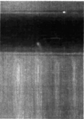
~---"'" -, ~ :!l:!l.j . ----:: --- . •i • ,:-.j ~tW " ''''- yl .,... -~.1

Figure 1-2: View of the gap cross-section of the low viscosity Boger fluid at De = 1.88,

Re

=

33.4 (co-rotating cylinders). Downwardly rolling vortices begin to form at 10

minutes. The direction of rotation of vortices along the inner cylinder is reveled by the

clockwise motion of the comma shaped region of seed depletion in the vortex visible from

40 to 44 minutes. Reproduced from [9].

from either end of the cylinders as though the cylinders were infinitely long. However, as we approach either end of the cylinders we will see effects from the shear on the top and bottom bounding surfaces. The existence of a bounding wall appears to cause effects to propagate throughout the fluid and cause flow cells to develop that are at first

three-dimensional steady and then become time-dependent as the viscoelasticity of the fluid is

increased. The cells have been shown to travel up and down the axis of the cylinders,

[9]. A time history of the formation of rolling cells of a Boger fluid within co-rotating cylinders is shown in Fig. 1-2.

(31)

Development of three dimensional structures from the growth of instabilities in the flow of viscoelastic fluids is in fact common throughout the literature. As shown by Evans and Walters ([31] and [32]) entry flows into a planar contraction of width to height ratio of 1 to 2 yields fully three-dimensional structures, another phenomena that could not possibly be captured with a two-dimensional simulation. Genieser [33] also explored the effects of contraction ratio on instabilities in the planar contraction. While the mechanism of the instability is not fully understood, it is apparent that the boundedness in the "neutral" direction is not likely the cause given that the instability exists for a wide range of width to height ratios. Another such instability that has been well studied is the flow around period array of cylinders of various inter-cylinder spacings [3], [71], [54],

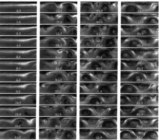
[57]. For the infinitely spaced case, that of an isolated cylinder in a channel, McKinley et al. [57] observed through experimentation three dimensional spatially periodic structures on the downstream side of the cylinder as illustrated in Fig. 1-3. Instabilities can also arise in unconfined flows such as those present in fiber spinning illustrated in Fig. 1-4. Here the flow is shown to progress from a stable column of fluid in (a), to a shark-skin instability starting in (b), and finally to gross melt fracture in (f) and (g).

Aside from the need for three-dimensional simulations to capture flow structures that arise from instabilities, there are also many industrially important problems in which the three-dimensional structure of the problem arises from the problem geometry, such as extrusion dies used in the fiber spinning industry and film casting industry. Traditional fiber spinning consists of extrusion and draw down of a cylindrical filament from a die. By assuming the filament and die are both axisymmetric, the model is reduced from three dimensions t;o two dimensions [71]. However, this is rarely the case in the fiber spinning industry. In some cases fibers of varying cross section are used to enhance properties such as touch and feel and even to enhance mass and heat transfer properties fabrics constructed of the fiber. Of all of the cross-sections pictured in Figs. 1-5 and 1-6, only the circular cross-section can be modeled by a two-dimensional axisymmetric simulation. The other fibers require three-dimensional simulations to capture the intricacy of the

(32)

Figure 1-3: Steady, spatially periodic structure of a Boger fluid flowing past an isolated

(33)

m~-

---'-.~'-~~.

<,.' '\..', J l I. ~---~-~~~:.Mltt ..'~A'''.JQ:.~~ ~t~~

.'

...

~ , ~~_-_-r_-t .::.'--.:..<"-:ccU"".~ ._

.

~rt~~.~25i;:;;'=_~

Figure 1-4: Example of an instability arising in the extrusion of a single strand polymer

filament. Steady flow is shown in (a), evolving into a shark-skin instability in (b)-(e),

and finally gross melt fracture in (f) and (g). Extrudates of a polymer melt at 70° C.

Shear rates are (a) 1.36S-l, (b) 2.72 s-1, (c) 6.81 s-1, (d) 13.6S-l. (e) 34.1 s-1, (f) 68.1

s-1, and (g) 136S-l. Fiber is roughly 1 mm in diameter. Reproduced from [88].

o

(34)

Figure 1-6: Artist rendition of a 4 DG Deep-Groove fiber. The cross-section is designed

to have enhanced capillary action allowing for improved wicking properties as well as

greatly increased surface to volume ratio over traditional fibers. Reproduced from [2]

, fiber cross-section.

Even in the case of circular cross section fibers, because of the high processing rates used in industry, it is common practice to draw multiple fibers from a single die assembly and then draw the fibers together into a bundle. Die plates with three, five, or more die

holes are used in these applications. While each die hole could behave as an independent

contraction flow at relatively low processing rates with isolated lip vortices [8], it is

unclear what would happen as the lip vortices from two adjacent die holes collide with

o

0 o

o

0

(35)

one another as the processing rates are increased. Certainly rich behavior beyond the modeling capacity of the two-dimensional case of the simple one-holed die is likely to occur.

It is clear that the need for three-dimensional modeling of the dynamics of viscoelastic fluids is important for the understanding and development of many applications. Work with the three-dimensional models to this point in the field has included mostly finite volume simulations on relatively coarse meshes as in [60], [87], and [89] with some at-tempts in finite elements on even coarser meshes [8]. More recently parallelization of the viscoelastic flow problem has been utilized to break up the calculation among a number of machines effectively reducing the overall time to reach solution or increasing the at-tainable calculation size. Application of a three-dimensional finite volume method can be found in [28] and that of a two-dimensional finite element method in [16].

1.2 Goals and Outline of Thesis

The overall goal of this body of work is to further develop the set of tools available for the analysis of viscoelastic flows. The main target for achievement of this goal is the development, a three-dimensional modeling package for viscoelastic flows. Due to the large set of equations that describe typical three-dimensional viscoelastic flow systems, it is necessary to develop numerical methods and formulations that pursue the solution to the viscoelasitc flow system in the most optimal manner. To aide in this effort, the methods developed in this thesis take advantage of the techniques developed in a well-documented two-dimensional finite element package in terms of formulation of the equations and parallel solution of the resulting set of differential algebraic equations. To further reduce the overall size of the set of differential algebraic equations, modification of the formulation of the equations was studied and documented herein. Also, since a comprehensive package in terms of the physical description of the system is of inter-est, the use of additional evolution equations for added physical description and for new

(36)

and diverse descriptions of the polymer stress is addressed. For example, incorporation of evolution equations describing the motion of free surfaces within the computational domain and incorporation of a closed form of the Adaptive-Length-Scale model for

im-proved description of the polymer stress are presented. Furthermore, since the size of the equation set resulting from sufficient refinement of the three-dimensional geometry

with a finite element mesh can be quite sizable when compared to its two-dimensional counterpart, development of optimal parallel solution techniques to divide up the set of equations among multiple processors is presented. Finally, the power of the three-dimensional package is demonstrated on a complex viscoelastic flow known to exhibit a time-dependent elastic instability.

Since the field of modeling and simulation of viscoelastic flows is well established, a significant amount of background study is helpful before proceeding. The first couple of chapters of this thesis are dedicated to aid the reader in this endeavor. Chapter 2 discusses the physics of viscoelastic fluids in simple and complex flows. The chap-ter begins with the description of some of the more inchap-teresting flow phenomena that has been observed by experimentalists. The simple flows typically used to measure the performance of models for viscoelastic fluids by comparison of the computed and ex-perimentally measured material functions are then described. Finally, the governing equations for viscoelastic fluid flow are given, starting with the conservation equations for the mass and momentum of the fluid and ending with continuum-based constitutive equations describing the relationship between the flow field and the stress of the fluid. While there have been a large number of constitutive equations developed over the history

of modeling of viscoelastic fluids, equations described herein are only those most relevant to the work contained within this document and their most relevant predecessors.

Chapter 3 further aids the reader in the understanding of viscoelastic fluid flow model-ing and simulation. This chapter is dedicated to the discussion of the numerical methods used to attack the daunting task of simulation of complex viscoelastic flows. The chapter begins with the description of the more recent history of the formulations of the

(37)

viscoelas-tic governing equations. The finite element method, the discretization workhorse in the field of viscoelastic flow simulation, is then discussed, with examples designed to help the reader understand how the governing equations are fit into this framework. The basis functions and elements are also included to help with understanding the implemen-tation of the finite element method. Next, a discussion is included of the decoupled sub-problem formulation of the time-dependent set of equations with comparison to the direct computation of the steady-state set of equations. A brief treatment of time in-tegration methods is included, with advantages and disadvantages of each given. The parallel solution method used within this work is then discussed in detail. Finally, to motivate the need for all of the advanced numerical methods included within this work,

a sample problem size calculation is included for a model fiber spinning problem taken

from the literature.

Chapter 4 is dedicated to the description of the decoupled velocity gradient inter-polant formulation. This is a new method designed at reducing the overall size of the computational problem by taking advantage of the time-dependent form of the equa-tions and the sub-problem formulation discussed in chapter 3. The chapter begins with discussion of the decoupled form of the equations and suggests two different forms of the equations used to compute the velocity gradient interpolant: a global least squares minimization and a local patch formulation. Measurement of the performance of these two formulations is presented in detail, the goal of which is to determine the method that provides the largest reduction in the overall problem size without loss of detail in the viscoelastic flow simulation. While the local patch formulation appears to offer great savings in overall problem size, as the Deborah number is increased, the velocity gra-dient field computed from the method deviates more and more from the accepted ideal of the fully coupled set of equations. To combat this increase in error, increased mesh refinement can be used, but at a significant cost to the overall calculation. The decou-pled global least squares minimization formulation on the other hand shows virtually no deviation from the ideal solution and requires no further mesh refinement. The chapter

(38)

concludes with a sample problem size calculation comparing the fully coupled method with both the decoupled least squares and the local patch formulations, demonstrating

the significant savings in problem size offered by the new decoupled global least squares formulation for the calculation of the velocity gradient interpolant.

Chapter 5 contains the development of the time-dependent free-surface viscoelastic finite element method for two-dimensional unconfined flows. The governing equations describing the flow of a viscoelastic fluid in an unconfined geometry are first presented. In addition to the governing equations given in the preceding chapters, the free-surface boundary conditions are now introduced along with the mapping equations used to up-date nodal positions in the deformable portion of the mesh. The numerical method used to attack this problem is then discussed, focussing on the implementation in the time-dependent, decoupled formulation. Though this development is carried out in the two-dimensional framework, it is intended to be applied to the full time-dependent, three-dimensional solver. The method outlined in this chapter is a demonstration of how an evolution equation describing some new physical aspect of the system is easily im-plemented in the decoupled, time-dependent formulation of the viscoelastic system of equations. Other equations that can be implemented in this manner included the en-ergy evolution equation and the crystallization kinetics evolution equation. As a test of the implementation of the free-surface governing equations, simulations of the die-swell of a Giesekus fluid emanating from a contraction die are compared to a known two-dimensional steady-state method for a range of Deborah numbers, Weisenberg numbers, and Capillary numbers. Excellent agreement is demonstrated between the two methods for all cases.

Chapter 6 contains the simulations of the flow of a Boger fluid in the 4:1:4 contraction-expansion geometry. The models used to represent the Boger fluid are the closed version of the Adaptive Length Scale model and the 4-mode FENE-P model. Use of these models within the time-dependent decoupled framework helps to demonstrate the variety of constitutive equations that can be easily implemented in this framework. The rheology

(39)

of the fluid characterized in [64] and [65] is modeled, and the comparisons to the key theological measurements are given in detail. The geometry used in the simulations is designed to model that used by Rothstein et al. [65]. The simulations of the flow in the 4:1:4 geometry with the ALS-C fluid model are the first to demonstrate pressure drop enhancement with increasing viscoelasticity, a well-known experimentally observed phenomenon. Qualitative growth of the vortex in the salient corner, parameterized

into radial and axial location of the vortex center, as well as the reattachment length also agrees qualitatively with experimental findings. The simulation with the 4-mode FENE-P model also shows pressure drop enhancement and salient corner vortex growth, but the simulations prove to be difficult to converge as the viscoelasticity increases and do not show the dramatic trends that the ALS-C model simulations exhibit.

Chapter 7 details the three-dimensional finite element package for viscoelastic flows in confined geometries. This package is based on the two-dimensional method used in chapters 4-6. It builds upon the time-dependent, decoupled formulation and takes ad-vantage of the decoupling of the velocity gradient interpolant equation as presented in chapter 4. 'To develop a method for robust use with many different physical geometries, implementation of a number of different boundary conditions was crucial. The boundary conditions implemented are given in detail. Next the elements and basis functions used in the three--dimensional package are given along with a description of the mesh genera-tion software used. To test the accuracy of the method, simulagenera-tions of Newtonian and Giesekus fluids flowing in pipe and duct geometries are compared to analytical solutions where available or otherwise to simulation generated from a well-tested two-dimensional method and to results published in the literature. Due to the large size of the finite element meshes needed to resolve flows in three-dimensional geometries, a parallel imple-mentation of the three-dimensional package is detailed. Favorable performance of the package is demonstrated for the duct flow problem with increasing parallel machine size. Chapter 8 contains simulations the flow of an Oldroyd-B fluid in a periodic, linear array of cylinders. The geometry is designed to match that used by Liu et al. [54] in

(40)

experimental identification a time-dependent instability of the flow of a Boger fluid and later used by Smith et al. [73] in a linear stability analysis of the flow. Comparisons are made of the flow fields and stress fields generated in an infinitely wide array described by a two-dimensional simulation and by a three-dimensional simulation with periodic boundaries on the side walls of the computational domain. The effects of adding solid side-walls to the geometry are also discussed. Finally, the flow structures arising in the infinite width array with a periodic computational domain of width 2, 3, and 4 units are explored and compared to the flow structure found by Smith et al..

Chapter 9 contains a summary of the work and results presented in this document. Finally, the author's views are included concerning the extensions of the work in this document and the possible exploitation of the techniques developed herein for further improving the simulation efforts for viscoelastic fluid flows.

(41)

Chapter 2 Physics of Viscoelastic Fluids

The physics associated with the flow of viscoelastic fluids is an area of research that is rich in interesting flow phenomena but is described by a set of governing equations that is difficult at best to solve. In this chapter, by way of justification of the above statement and as motivation into why the area of viscoelastic fluids is one of interesting research, some of the flow phenomena are first presented to give the reader a feel for the unique behavior of viscoelastic fluids in flow as compared to flows of the relatively simple Newtonian fluids. Simple flows that are commonly used to characterize the rheology of the viscoelastic fluids are then described. Finally, the equations governing the flow of viscoelastic fluids are presented.

2.1 Flow Phenomena

Many interesting and visually stimulating phenomena have been observed in the flow of fluids. A number of books are available with a broad array experimental visualizations from fluid flow. For phenomena focused mostly in the area of Newtonian flows, the reader is directed to the book assembled by Van Dyke [84]. An excellent collection of experimental visualizations for viscoelastic fluid flows is that compiled by Boger and Walters [12]. Here a few examples of the phenomena of viscoelastic flows that differ

Analysis of complex viscoelastic flows using a finite element method

Analysis of Complex Viscoelastic Flows Using a

Finite Element Method

bv

Scott David Phillips

Su11)l1ut

t,('d to te Department of Chemnlical

Engineering

in partial flfillment of the requirenments for the egree of

Doc:tor of Philosophy

at the

February 2006

®

NhMassachlset

l.s Institute of Technology 2006

Signat

ure

of

Autho1

Department of

Chemic:al Engineering

Professor of

Robert A. Brown

(]henieal Engineering

T

hesis Supervisor

Professor of

Robert C. Arnst rong

Chemical Engineering

Thesis Spplervisor

... .. ...

William N*. Deen

II

ItLAPi

Analysis of Complex Viscoelastic Flows Using a Finite Element

Method

by

Scott David Phillips

Abstract

Contents

...

...

...

...

...

List of Figures

ele-ment

.. ... . ... 89

IHrfll

I:

0:

/

/3

/3

3

3

3

3

/3

3

3

List of Tables

Chapter 1

Introduction

1.1 Motivation

----

=

m~-

---'-.~'-~~.

.'

...

.

o

o

0

o

o

0

1.2 Goals and Outline of Thesis

Chapter 2