HAL Id: inserm-00131803
https://www.hal.inserm.fr/inserm-00131803
Submitted on 19 Feb 2007HAL is a multi-disciplinary open access archive for the deposit and dissemination of sci-entific research documents, whether they are pub-lished or not. The documents may come from teaching and research institutions in France or
L’archive ouverte pluridisciplinaire HAL, est destinée au dépôt et à la diffusion de documents scientifiques de niveau recherche, publiés ou non, émanant des établissements d’enseignement et de recherche français ou étrangers, des laboratoires
Frequency and phase contributions to the detection of
temporal luminance modulation.
James Thomas, Kenneth Knoblauch
To cite this version:
James Thomas, Kenneth Knoblauch. Frequency and phase contributions to the detection of temporal luminance modulation.. J Opt Soc Am A Opt Image Sci Vis, 2005, 22 (10), pp.2257-61. �inserm-00131803�
Frequency and phase contributions to the
detection of temporal luminance modulation
James P. Thomas
Psychology Department, UCLA, Box 951563, Los Angeles CA 90095-1563, USA
Kenneth Knoblauch
Inserm U371, Cerveau et Vision, Dept. of Cognitive Neurosciences, IFR19, UCB –
Lyon 1, 18 avenue du Doyen L´epine, 69675 Bron cedex, France
HAL author manuscript inserm-00131803, version 1
HAL author manuscript
Observers detected a temporally modulated luminance pattern embedded
in dynamic noise. A Gabor function with a carrier frequency, in separate
conditions of 0, 1.56, or 3.12 Hz, modulated signal contrast. Classification
images were constructed in the time, temporal frequency, and temporal phase
domains. As stimulus frequency increased, amplitudes of the phase images
decreased and amplitudes of the frequency images increased, indicating a
corresponding shift in the observers’ criteria. The reduced use of phase
attenuated time domain images from signal-absent trials, but physical
inter-actions between signal and noise components tended to preserve time domain
images from signal present trials. The results illustrate a frequency-dependent
strategy shift in detection that may reflect a degree of stimulus uncertainty
in the time domain. 2005 Optical Society of Americac
OCIS codes: 330.1880, 330.4060, 330.6790
1. Introduction
The visual system does not simply generate a neural replica of a stimulus, but codes
and separately represents various components of it. DeValois and his students took a
leading role in characterizing the neural mechanisms underlying such separate
repre-sentations. Chromatic and luminance differences are coded early in segregated
path-ways,1, 2 and neurons in primary visual cortex are selectively sensitive or tuned with
respect to a variety of spatial and temporal properties.3–5 Such selectivities provide
the basis for separate representations and processing of the information coded in the
neural responses.3–8 One goal of psychophysics is to understand how these different
representations are weighted and combined in the performance of various
percep-tual tasks. In this research, we exploit classification images to understand better how
observers employ different temporal properties in a visual detection task.
Confusions have long been a source of information about the stimulus properties
important to the performance of perceptual tasks. Ahumada9, 10 refined this approach
by embedding auditory signals in noise and comparing the noise profiles that increased
the probability of “present” responses with the noise profiles that increased the
prob-ability of “absent” responses. He termed the difference between these two types of
profiles, which he analyzed in the temporal frequency domain, the classification
im-age. More recently, Ahumada and others have used the technique to investigate the
stimulus properties used in a variety of visual tasks, (See reference11 for a recent
overview.). We here describe the classification images found for the task of detecting
a temporally modulated luminance pattern in temporally dynamic luminance noise,
with particular attention to how the images change with the rate of signal
modula-tion. A preliminary report was presented at the 1999 meeting of the Association for
Research in Vision and Ophthalmology.12
Our observers detected a temporal Gabor signal embedded in temporally dynamic
noise. In different conditions, the carrier signal of the Gabor varied from 0 Hz to
3.12 Hz. We formed classification images in the time, temporal frequency, and
tempo-ral phase domains. The forms and amplitudes of the images changed with the carrier
frequency in a way that suggested that temporal phase information became less
im-portant and temporal frequency information more imim-portant as carrier frequency
increased. The results demonstrate the utility of constructing images in all relevant
domains.
2. Methods
The stimulus set-up has previously been described in detail.13In brief, all stimuli were
presented on an Eizo FlexScan T562-T color monitor driven by software on a PC
com-puter under the control of a Cambridge Research Systems (CRS) VSG/2 color
graph-ics card that provides 12 bits of resolution for each phosphor of the 800 × 600 pixel
display. The screen was run at a field rate of 100 Hz, non-interlaced. The
voltage-phosphor luminance relationship was linearized with look-up tables. Calibration of the
screen was performed with a Minolta CS-100 chromameter and a silicone photo-diode
used with the OPTICAL software (CRS). The screen was set to a steady background
with luminance 65 cd/m2 and chromaticity (0.294, 0.303) for the CIE 1931 standard
observer.
Observers detected a temporally modulated luminance signal embedded in dynamic
luminance noise. The stimulus presented on each trial was the product of a spatial
modulation function and a temporal modulation function. The spatial function was a
2D Gaussian with a standard deviation (σ) of 2.4 degrees. On signal-present trials, the
temporal function was the sum of a Gabor function and a noise vector, both sampled
at 50 Hz. On signal-absent trials, only the noise vector modulated the target. The
Gabor function was the product of a positive-going Gaussian window and a sinusoid.
The window had a σ of 160 ms and was truncated at plus and minus two σ’s, yielding
a stimulus duration of 640 ms. In different conditions, the temporal frequency of the
sinusoid was 0 (i.e., the window multiplied by a positive DC shift), 1.56 or 3.12 Hz.
These Gabor functions are shown in the upper left corner image of Figures 1, 2
and 3, respectively. Each noise vector consisted of 32 independent samples from a
uniform random distribution varying symmetrically about zero. The stimuli were
viewed binocularly from 57 cm.
Each session comprised 224 trials, evenly divided between present and
signal-absent trials. At the end of each stimulus presentation the observer indicated that the
Gabor signal was present or absent by pressing a key. Auditory feedback followed the
response. Each observer completed 16 sessions, distributed over at least four days, in
each condition. All sessions in one condition were completed before proceeding to the
next condition. For both observers, the order of conditions was 0, 1.56 and 3.12 Hz.
Noise power (1/3 contrast2) was 0.03 for all conditions. Signal contrast, measured
at the peak of the envelope, was separately set for each observer and condition to
yield a d0 near 1.0. The contrasts for the 0, 1.56, and 3.12 conditions, respectively,
were 0.07, 0.15 and 0.15 for observer KK, and 0.08, 0.21 and 0.18 for observer JPT.
Hit rates varied between 0.71 and 0.75, and false alarm rates varied between 0.28 and
0.37.
The two authors served as observers but remained naive as to the results until
data collection from both observers was completed. KK is emmetropic and JPT was
corrected for the viewing distance.
2.A. Classification Images
The noise vector from each trial was labeled as to type of trial (signal-present or
signal-absent) and the observer’s response (“present” or “absent”) and stored.
Dur-ing analysis, the noise records were segregated into four groups: hits
(trial=signal-present, response=present); misses (trial=signal-(trial=signal-present, response=absent); false
alarms (trial=noise only, response=present); and correct rejections
(trial=signal-absent, response=absent). The classification images were constructed from these noise
records.
2.B. Time Domain Images
Each noise record was smoothed by averaging each entry, beginning with the second,
with the previous entry. For each session, a mean vector was computed for each of the
four groups: hits, misses, false alarms, and correct rejections. Two session images were
computed for each session. A signal-present image was computed by subtracting the
mean vector for misses from the mean vector for hits, and a signal-absent image was
computed by subtracting the mean vector for correct rejections from the mean vector
for false alarms. These two types of session images were then averaged over sessions
and standard errors of the resulting mean images computed from the variability over
sessions. Individual points in the images were converted to z-scores by dividing each
mean by its standard error. Columns 2 and 3 of the first row of Figures 1–3 display
the z-score images.
Analyses of variance were conducted on session images computed without the initial
smoothing. A within subject analysis was conducted on the 16 sets of session images
for each subject and each condition. The factors were time and trial type
(signal-present or signal-absent). The presence of a reliable image was tested by the main
effect for time. The difference between signal-present and signal-absent images was
tested by the time-by-trial-type interaction. When a difference was found, each image
was separately tested for the presence of a signal component. When the analysis found
a reliable image, the agreement between the image and the luminance profile of the
stimulus was quantified by a correlation coefficient.
2.C. Temporal Frequency and Phase Domain Images
Each noise record was fast-Fourier transformed using the Matlab fft function. The
temporal frequency spectrum of the record was extracted from the fft output using the
Matlab abs function, and the phase spectrum was extracted with the angle function.
The transformed records of each type were segregated into groups corresponding to
hits, misses, false alarms, and correct rejections. Session means were computed as
described above and session images calculated by subtracting the mean spectrum for
misses from the mean spectrum for hits, in the case of signal-present trials, and by
subtracting the mean spectrum of correct rejections from the mean spectrum for false
alarms, in the case of signal-absent trials. These two types of session images were then
averaged over sessions and standard errors of the resulting mean images computed
from the variability over sessions. Individual points in the images were converted to
z-scores by dividing each mean by its standard error. Columns 2 and 3 of the bottom
two rows of Figures 1–3 display the z-score images.
The computation of z-scores for phase preserves sign, but the scores are not
con-strained to lie between ±π. Thus, it is the relative profile of the z-score images,
particularly with respect to modulations above and below zero, that is meaningful.
For example, if an observer used the correlation between the phase spectrum of the
signal and the phase spectrum of the stimulus (either noise-only or noise-plus-signal)
as the decision variable, the z-score image would mirror the sign of the spectrum of
the signal, but not match its values. More generally, reliable modulation of the
z-score phase image indicates that the observer used phase information in the decision
process.
2.D. Simulated observer
An observer who bases his judgments only on magnitude information was simulated
using the R statistical computing environment.14 A set of 3584 stimuli (16 sessions
of 224 trials) was generated with the same characteristics as those used to test the
human observers. Each stimulus was composed of 32 samples. Half of the trials were
composed of only noise, the others of signal plus noise. The noise was drawn from a
uniform distribution with power=0.03, and the signal was a Gabor whose Gaussian
envelope had a σ equal to 8 samples and sinusoidal carrier a frequency equal to (2σ)−1.
The contrast of the Gabor was set at 0.15. The magnitude spectrum of each stimulus
was extracted using the fft() function of R. The decision variable was calculated from
the dot product of the magnitude spectrum of the stimulus with that of the signal.
When the decision variable was greater than a criterion value of 0.45, the trial was
classified by the observer as present, otherwise as absent. These conditions generated a
d0 = 1.3 with the proportion of hits and false alarms equal to 0.8 and 0.3, respectively.
The time domain samples (not their magnitude spectra) were sorted into response
categories (hits, false alarms, etc.), averaged and combined to obtain present and
absent classification images.
3. Results
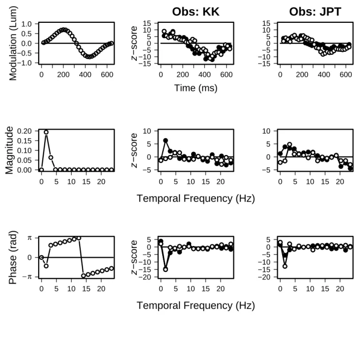
Figure 1 presents the classification images from the 0 Hz condition. Both subjects have
well defined images in the time domain, with images derived from signal-present trials
and from signal-absent trials agreeing closely. KK’s images resemble the luminance
profile of the signal, although somewhat skewed toward higher values in the latter
half, while JPTs images are oppositely skewed, with higher values in the first half of
the stimulus epoch. The correlations between the luminance profile of the signal and
the individual images range from 0.71 to 0.78.
In the Fourier domains, both observers have sharply defined phase images consisting
of a single, negative-going lobe. Relative to the phase spectrum of the signal, the lobe
is shifted toward lower temporal frequencies. The images derived from signal-present
and from signal-absent trials agree closely. In the magnitude domain, however, the
images are less clear-cut. At the lowest temporal frequency, the signal-present images
for both observers are negative. Since magnitudes are positive, the negative values
mean that the presence of noise components at this frequency biased the observers
toward an “absent” response. When the signal was absent, these same components
biased observer KK toward a “present” response and had little effect on the response
of JT. At higher frequencies, the data points of KK’s image hover around zero, while
those of JT suggest low amplitude peaks at 1.56 Hz.
Figure 2 presents the images from the 1.56 Hz condition. Again, both observers
have well defined images in the time domain. The images from signal-present and
signal-absent trials resemble each other, but the slight differences are statistically
significant (p < 0.01 for KK, p < 0.05 for JPT). The images derived from the
signal-present trials correlate more closely with the luminance profile of the signal (0.81 vs
0.80 for KK, 0.94 vs 0.78 for JPT).
In the Fourier domains, both observers have sharply defined phase images consisting
of single, negative-going lobes at the peak temporal frequency of the stimulus. The
signal-present and signal-absent images of KK are essentially coincident, but the
signal-absent image of JPT has less amplitude than his signal-present image. In the
magnitude domain, the signal-absent image of KK peaks at the temporal frequency
of the signal, but his signal-present image is essentially flat. The signal-present image
of JPT has a single peak that occurs at a higher temporal frequency than the signal.
His signal-absent image is broad and of lower amplitude.
Figure 3 presents images from the 3.12 Hz condition. The time domain images of
KK differ between signal-present and signal-absent (p < 0.001). The signal present
image is skewed toward higher amplitude in the second half of the stimulus epoch,
but the correlation with the signal profile remains high (0.83). The signal-absent
image is nearly flat, but does contain a significant signal component (correlation =
0.63). The signal-present and signal-absent images of JPT also differ from each other
(p < 0.001). The correlation between the luminance profile of the signal and the
signal-present image is 0.87. The signal-absent image is flat and does not contain a
significant signal component.
In the Fourier domains, the magnitude images of both observers have greater
am-plitudes than in the other two conditions. The present images are broadly tuned and
peak at a lower temporal frequency than the peak frequency of the signal. For both
observers, the signal-absent image has greater amplitude than the signal-present
im-age. Just the opposite relationship occurs in the phase images: for both observers,
the phase image from signal-present trials has greater amplitude, and more closely
resembles the profile of the phase spectrum of the signal, than the image derived from
signal absent trials. The signal-absent phase image for JPT is essentially flat.
4. Discussion
The presence of a classification image, particularly from signal-absent trials, indicates
that the property represented plays a significant role in the observer’s decision process.
Since performance levels were constant across conditions, changes in the classification
images from one condition to another reflect changes in the observer’s use of stimulus
information.
One such shift is in the balance between the use of temporal frequency and temporal
phase information. In the 0 Hz condition, the phase domain images are narrowly
defined and of high amplitude, while the temporal frequency domain images are less
well defined and of lower amplitude. In the 3.12 Hz condition, on the other hand,
it is the frequency images which are more clearly defined and of higher amplitude,
particularly on signal-absent trials. These changes support a conclusion that decision
processes emphasized phase in the low frequency condition, but that flicker rate,
perhaps without regard to phase, was emphasized in the high frequency condition.
The results should not be taken to mean that observers totally ignored temporal
frequency information in the lower modulation conditions: the narrowness of the phase
images on the frequency axis indicates that the selective use of phase information was
restricted to the frequency region of the signal.
The reduced use of phase information provides one reason for the difference
be-tween time domain images from signal-present and signal-absent trials in the 3.12 Hz
condition. When the signal is present, any noise component similar in temporal
fre-quency and phase to the signal will increase the effective contrast of the signal and
strengthen the representations of both temporal frequency and phase information.
As a result, the decision process is biased toward responding “present” even if only
frequency information is used and phase information ignored. However, if the noise
component is out of phase with the signal, the effective contrasts of the signal and of
the noise component are reduced, as are the representations of frequency and phase,
and the decision is biased toward “absent.” As a result of this interaction, the time
domain image from signal-present trials tends to mirror the signal and a phase
do-main image may appear even though the decision processes ignore phase per se. When
the signal is absent, on the other hand, the strength of the temporal frequency
rep-resentation depends only on the frequency content of the noise and not on phase.
Because the phase relationships in the noise vary randomly, averaging the noise
pro-files over trials tends to produce flat images in the time and phase domains. Figure 4
presents the time domain classification images of a simulated observer who uses only
frequency information, i.e. who uses the correlation between the magnitude spectra
of the signal and of the stimulus (noise-only or noise-plus-signal) as the decision
vari-able. Consistent with the argument just given, there is a clear difference between the
simulated signal-present and signal-absent images: the signal-present image mirrors
the temporal profile of the signal, while the signal-absent image is flat.
Solomon15 obtained analogous results in spatial domains. When observers sought
to detect a peripherally presented spatial grating, signal-present trials yielded a space
domain classification image, but signal-absent trials did not. However, both types of
trials yielded images in the spatial frequency domain. Solomon inferred that observers
used information about spatial frequency, but not about spatial phase, in their
de-cision processes. In a separate condition, Solomon found evidence that the effect of
noise components on signal contrast was a major determinant of observers’ responses
on signal-present trials.
Several investigators have noted and discussed differences between classification
im-ages derived from signal-present and signal-absent trials (e.g.9, 16–20), and the
consen-sus is that such differences argue against completely linear decision models. Stimulus
uncertainty, in the spatial or temporal domain, has been proposed as one possible
source of the differences, and this suggestion has been supported by modeling
re-sults.18, 21 With respect to the present findings, temporal uncertainty may underlie
the changing roles of temporal phase and temporal frequency information as signal
frequency increased. A given uncertainty in the time domain translates into a phase
uncertainty that increases in proportion to signal frequency. Thus, a temporal
un-certainty that might have little effect on phase information in the 0 Hz condition
might have substantial effect in the 3.12 Hz condition, leading observers to place
more emphasis on frequency information.
These and other results, such as those of Solomon, illustrate the potential of
clas-sification images to increase our understanding of the manner in which the visual
system abstracts information about separate stimulus properties and about how
de-cision processes use the representations of these properties in perceptual judgment.
Acknowledgements
JPT’s participation was supported by a visiting professorship from the Universit´e
Jean Monnet, Saint ´Etienne, France.
References
1. R. L. DeValois, I. Abramov, and G. H. Jacobs, “Analysis of response patterns of
LGN cells,” J. Opt. Soc. Am. 56, 966–77 (1966).
2. R. L. DeValois, “Some transformations of color information from lateral geniculate
nucleus to striate cortex,” Proc. Natl. Acad. Sci. USA 97, 4997–5002 (2000).
3. R. L. DeValois, E. W. Yund, and N. Hepler, “The orientation and direction
se-lectivity of cells in macaque visual cortex,” Vision Res. 22, 531–544 (1982).
4. R. L. DeValois, D. G. Albrecht, and L. G. Thorell, “Spatial frequency selectivity
of cells in macaque visual cortex,” Vision Res. 22, 545–559 (1982).
5. R. L. DeValois, N. P. Cottaris, L. E. Mahon, S. D. Elfar, and J. A. Wilson,
“Spa-tial and temporal receptive fields of geniculate and cortical cells and directional
selectivity,” Vision Res. 40, 3685–3702 (2000).
6. J. A. Movshon, E. H. Adelson, M. S. Gizzi, and W. T. Newsome, “The
analy-sis of moving visual patterns,” in Pattern Recognition Mechanisms, C. Chagas,
R. Gattass, and C. Gross, eds., pp. 117–151 (Springer, New York, 1985).
7. L. A. Olzak and J. P. Thomas, “Neural recoding in human pattern vision: model
and mechanism,” Vision Res. 39, 231–256 (1999).
8. S. Magnussen and M. W. Greenlee, “The psychophysics of perceptual memory,”
Psychol. Res. 62, 81–92 (1999).
9. A. J. Ahumada, Jr., “Detection of tones masked by noise: A comparison of
hu-man observers with digital-computer-simulated energy detectors of varying
band-widths,” Ph.D. thesis, University of California, Los Angeles (1967).
10. A. J. Ahumada, Jr. and J. Lovell, “Stimulus features in signal detection,” J.
Acoust. Soc. Am. 49, 1751–1756 (1971).
11. M. P. Eckstein and A. J. Ahumada, Jr., “Classification images: A tool to
analyze visual strategies,” J. Vision 2, i–i, http://journalofvision.org/2/1/i/,
doi:10.1167/2.1.i, (2002).
12. K. Knoblauch, J. P. Thomas, and M. D’Zmura, “Feedback, temporal frequency,
and stimulus classification,” Invest. Ophth. Vis. Sci. 40, S792 (1999).
13. M. D’Zmura and K. Knoblauch “Spectral bandwidths for the detection of color,”
Vision Res., 38, 3117–3128 (1998).
14. R Development Core Team (2004). “R: A language and environment for statistical
computing”. R Foundation for Statistical Computing, Vienna, Austria. ISBN
3-900051-07-0, URL http://www.R-project.org.
15. J. A. Solomon, “Noise reveals visual mechanisms of detection and
discrimina-tion,” J. Vision 2, 105–120, http://journalofvision.org/2/1/7/, doi:10.1167/2.1.7,
(2002).
16. B. L. Beard and A. J. Ahumada, Jr., “A technique to extract relevant image
features for visual tasks,” in Human Vision and Electronic Imaging III, SPIE
Proceedings 3299, B. E.Rogowitz and T. N.Pappas, eds., pp. 79–85 (1998).
17. A. J. Ahumada, Jr. and B. L. Beard, “Classification images for detection,” Invest.
Ophth. Vis. Sci. (40), S572 (1999).
18. E. Barth, B. L. Beard, and A. J. Ahumada, Jr.,“Nonlinear features in vernier
acuity,” in Human Vision and Electronic Imaging IV, SPIE Proceedings 3644,
B. E.Rogowitz and T. N.Pappas, eds., pp. 88–96 (1999).
19. A. J. Ahumada, Jr.,“Classification image weights and internal noise level
estima-tion,” J. Vision 2, 121–131, http://journalofvision.org/2/1/8/, doi:10.1167/2.1.8,
(2002).
20. C. K. Abbey and M. P. Eckstein, “Classification image analysis: Estimation and
statistical inference for two-alternative forced-choice experiment”. J. Vision 2,
66–78, http://journalofvision.org/2/1/5/, doi:10.1167/2.1.5, (2002).
21. R. F. Murray, P. J. Bennett, and A. B. Sekuler, “Classification images
dict absolute efficiency,” J. Vision 5, 139–149, http://journalofvision.org/5/2/5/,
doi:10.1167/5.2.5, (2005).
List of Figure Captions
Fig. 1. Classification images for the 0 Hz condition. The first row shows images in
the time domain; the second row shows images in the temporal frequency domain;
and the third row shows images in the temporal phase domain. Column 1 shows
the luminance modulation profile and spectra of the Gabor signal. Columns 2 and
3 show the classification images for observers KK and JPT, respectively. Each data
point is a z-score, calculated as described in Methods. White symbols calculated from
signal-present trials; black symbols calculated from signal-absent trials.
Fig. 2. Classification images for 1.56 Hz condition. See legend for Figure 1.
Fig. 3. Classification images for 3.12 Hz condition. See legend for Figure 1.
Fig. 4. Simulated time domain images, in the 3.12 Hz condition, for an observer who
uses only frequency information. The decision variable is the correlation between the
magnitude spectrum of the signal and the magnitude spectrum of the stimulus. White
symbols calculated for signal-present trials; black symbols calculated for signal-absent
trials.
0 200 400 600 0.2 0.4 0.6 0.8 1.0
Modulation (Lum)
0 200 400 600 0 5 10 15Obs: KK
Time (ms)
z
−score
0 200 400 600 0 5 10Obs: JPT
0 5 10 15 20 0.0 0.1 0.2 0.3 0.4Magnitude
0 5 10 15 20 −10 −5 0 5 10z
−score
Temporal Frequency (Hz)
0 5 10 15 20 −5 0 5 10 0 5 10 15 20Phase (rad)
− π − π 2 0 0 5 10 15 20 −20 −15 −10 −5 0z
−score
Temporal Frequency (Hz)
0 5 10 15 20 −20 −15 −10 −5 0Fig. 1. Classification images for the 0 Hz condition. The first row shows images
in the time domain; the second row shows images in the temporal frequency
domain; and the third row shows images in the temporal phase domain.
Col-umn 1 shows the luminance modulation profile and spectra of the Gabor signal.
Columns 2 and 3 show the classification images for observers KK and JPT,
respectively. Each data point is a z-score, calculated as described in Methods.
White symbols calculated from signal-present trials; black symbols calculated
0 200 400 600 −1.0 −0.5 0.0 0.5 1.0
Modulation (Lum)
0 200 400 600 −15 −10−5 0 5 10 15Obs: KK
Time (ms)
z
−score
0 200 400 600 −15 −10−5 0 5 10 15Obs: JPT
0 5 10 15 20 0.00 0.05 0.10 0.15 0.20Magnitude
0 5 10 15 20 −5 0 5 10z
−score
Temporal Frequency (Hz)
0 5 10 15 20 −5 0 5 10 0 5 10 15 20Phase (rad)
− π 0 π 0 5 10 15 20 −20 −15 −10 −5 0 5z
−score
Temporal Frequency (Hz)
0 5 10 15 20 −20 −15 −10 −5 0 5Fig. 2. Classification images for 1.56 Hz condition. See legend for Figure 1.
0 200 400 600 −1.0 −0.5 0.0 0.5 1.0
Modulation (Lum)
0 200 400 600 −20 −10 0 10 20Obs: KK
Time (ms)
z
−score
0 200 400 600 −20 −10 0 10 20Obs: JPT
0 5 10 15 20 0.00 0.05 0.10 0.15 0.20Magnitude
0 5 10 15 20 −5 0 5 10 15z
−score
Temporal Frequency (Hz)
0 5 10 15 20 −5 0 5 10 15 0 5 10 15 20Phase (rad)
− π 0 π 0 5 10 15 20 −10 −5 0 5 10z
−score
Temporal Frequency (Hz)
0 5 10 15 20 −10 −5 0 5 10Fig. 3. Classification images for 3.12 Hz condition. See legend for Figure 1.
0
200
400
600
−20
−10
0
10
20
Time (ms)
z
−score
Fig. 4. Simulated time domain images, in the 3.12 Hz condition, for an observer
who uses only frequency information. The decision variable is the correlation
between the magnitude spectrum of the signal and the magnitude spectrum of
the stimulus. White symbols calculated for signal-present trials; black symbols
calculated for signal-absent trials.