Numerical analysis of frost effects in porous media. Benefits and limits of the finite element poroelasticity formulation

HAL Id: hal-01724657

https://hal.insa-toulouse.fr/hal-01724657

Submitted on 23 Mar 2018

HAL is a multi-disciplinary open access

archive for the deposit and dissemination of sci-entific research documents, whether they are pub-lished or not. The documents may come from teaching and research institutions in France or abroad, or from public or private research centers.

L’archive ouverte pluridisciplinaire HAL, est destinée au dépôt et à la diffusion de documents scientifiques de niveau recherche, publiés ou non, émanant des établissements d’enseignement et de recherche français ou étrangers, des laboratoires publics ou privés.

Numerical analysis of frost effects in porous media.

Benefits and limits of the finite element poroelasticity

formulation

Stéphane Multon, Alain Sellier, Bernard Perrin

To cite this version:

Stéphane Multon, Alain Sellier, Bernard Perrin. Numerical analysis of frost effects in porous media. Benefits and limits of the finite element poroelasticity formulation. International Journal for Numerical and Analytical Methods in Geomechanics, Wiley, 2012, 36 (4), pp.438-458. �10.1002/nag.1014�. �hal-01724657�

Numerical analysis of frost effects in porous media.

Benefits and limits of the finite element poroelasticity

formulation

Stéphane Multon

*

_{, Alain Sellier}

_{, Bernard Perrin}

Université de Toulouse ; UPS, INSA; LMDC (Laboratoire Matériaux et Durabilité des Constructions); 135, avenue de Rangueil; F-31 077 Toulouse Cedex 04, France

Abstract

The aim of this paper is to analyse the performance of a finite element formulation usable to predict the mechanical consequences of frost effects on porous media. It considers the characteristics of porous media and how the frost action can be assessed. The problem is then separated into two parts: thermal and poromechanical calculations. The constitutive equations developed in the framework of poromechanics are presented and the implementation in a usual finite element poroelasticity formulation based on Zuber’s method is adopted. An analysis of the time-step influence on the convergence rate is given and leads us to propose a simple method in order to obtain objectivity of the finite element response and avoid over-long calculations. Frost effect simulations are carried out on real porous media (two fired clays) as a case study. Although the experimental behaviour of the porous media subjected to frost action is in accordance with some observations, the calculated strains appear to be overestimated compared to measurements. The problem could be largely attributable to the difficulty of assessing permeability evolution during frost development.

Key Words: Freeze, frost durability, pore size distribution, poroelasticity, porous media

1. Introduction

The development of ice in porous media such as cement-based materials [1-5] or fired clay materials [6-9] and its mechanical consequences have been largely investigated in order to understand the mechanisms and predict the frost resistance of materials. The problem is usually divided into two parts: the formation of the ice in the porous medium and the effect of this formation on the material (deformation and damage). In porous media, the formation of ice is driven by the conditions of equilibrium between vapour, water and ice, which are influenced by the curvature of their interfaces, the presence or absence of ionic species in the water, and the pressures applied to the phases [1, 2, 10-12]. The deformations of the porous medium during ice formation are the combined effect of different processes [13, 14]. Due to the temperature evolution, the porous material is affected by thermal contraction. Moreover, below the melting temperature, ice crystals develop. The 9% expansion due to the transformation of liquid water into ice is the cause underlying several mechanisms: such expansion in a porous medium causes internal stresses in the material and causes an increase of the water pressure in the porosity of the material, which drives the liquid water out of the freezing sites. Finally, as the temperature continues to decrease, the cryo-suction effect drives water towards frozen sites [13, 14].

The aim of this paper is to present a modification of the usual finite element poroelasticity formulation to perform calculations based on an existing model [15, 16]. This model was developed in the framework of poromechanics [17] and was based on earlier works [12, 13, 18]. Zuber’s model has two interesting characteristics. First, it proposes to determine the ice development and the ice pressure on the pore walls from the pore size distribution. Most finite element codes use only the liquid pressure as the variable and do not allow the use of a second pressure variable. The second characteristic of this model is to take account of the different mechanisms due to ice formation by their effects on only the liquid water pressure. Thus, the ice pressure can be taken into account via the liquid water pressure, which allows most of the finite element codes to be used to program this model.

The characteristics of porous media subjected to frost action are described first: characteristics relative to the drained porous media (subscript 0) and to the three phases (liquid water l, ice i and solid s), determination of the ice development and assessment of the action of the ice crystals on the pore walls. The constitutive equations of the thermal and poromechanical problems are then presented in the framework of porous media subjected to frost action. In this paper, the thermal and the mechanical problems are considered as weakly coupled [15, 19]. Numerical considerations describe how the terms due to frost action can be taken into consideration in the usual finite element poroelasticity formulation and propose a method to perform objective calculations. The last part presents analyses performed on two real porous media (fired clays). The capability of the calculations to predict the measurements is then discussed.

2. Porous media subjected to frost action

2.1 Characteristics of porous media and phases

In order to perform reliable calculations on porous media, a good description of several physical parameters is necessary. First, the porosity has to be well known. In this paper, the cumulative volume of pores with a radius greater than r is defined by:

( )

=

∫

∞ r dr dr d r ϕ ϕ (1)

where ϕ represents the porosity of the pores with radius upper than r of the porous medium. The total porosity is:

∫

∞ = 0 dr dr d n ϕ (2)

In the calculations developed here, it is assumed that the porosity is saturated by liquid water l and ice i. Si is the volumetric fraction of the porosity filled by the ice and Sl is the fraction of

the porosity filled by the water. Therefore:

( )

T +S

( )

T =1

S_{i l} (3)

In order to assess the response of the porous media to frost action, the mechanical behaviour of the material has to be known. It can be characterized by an isotropic bulk modulus:

(

0

)

0 0 2 1 3 − ν = E K (4)

where E0 and ν0 are the elastic modulus and the Poisson coefficient of the drained porous

material.

The bulk modulus of solid grain is linked to the total porosity and to the bulk modulus of the drained porous medium. In this paper, the relationship proposed by Zuber and Marchand is used [15]:

(

)

3 0 1 n K K_s − = (5)

Finally, the Biot coefficient related to the liquid water is:

s

K K

b=₁− 0 (6)

2.2 Development of ice crystals in porous media

The conditions of equilibrium between liquid water and ice in saturated porous media are influenced by the curvature of the interfaces and the pressures applied to the phases [1, 2, 11, 12]. Therefore, the transformation of the liquid water into ice is not an instantaneous phenomenon even if the temperature is below 0°C in the whole of the porous medium. Relations between freezing or melting point and pore diameter of the material depend on the kinetics of freezing and thawing and are difficult to obtain. In this paper, the relation is assumed to be based on the equilibrium between the phases deduced from thermodynamic models [12-14]. Thus, the smallest curvature radius of an ice crystal that can be formed at a given temperature, T, can be deduced from Eq 7 (as illustrated in Figure 1):

( )

₍

( )

₎

T T T T R m M li eq − Σ = 2γ (7)

with γli, the surface tension of the liquid/ice interface, ΣM, the melting entropy, T the

temperature of the medium and Tm, the temperature of the melting point (Tm = 273 K) [13].

The value of γli and ΣM are given in the ‘Application’ section. ΣM is assumed to be constant

[12-14].

Moreover, in porous media, a part of the water is adsorbed on the pore walls and cannot freeze. This adsorbed water can be represented by a layer of water whose thickness depends on the temperature. Fagerlund proposed the following empirical relation [20]:

( )

1.97 3 1 T T T m − = δ (in nm) (8)

with δ the thickness in nm (Figure 1).

Therefore, the part of the porosity filled by the ice is composed of the pores of radius larger than:

( )

T R

( ) ( )

T T

R_Peq = _eq +δ (9)

During the calculations, the part of the porosity filled by liquid water and the part filled by ice have to be known. The water adsorbed on the pores walls forms part of the liquid water. In order to assess the volume of the adsorbed water, it is necessary to make an assumption on the shape of the pores. In the assumption of cylindrical pores, the relative volume of adsorbed water in a pore of radius r≤R_Peq(T) is given by:

( )

, 1 1

( )

2      − − = r T T r g δ (10)

with δ the thickness of the layer of the adsorbed water.

Therefore, the variation of the volume filled by the ice between two time steps t and t+dt depends on the related temperature evolution T(t) to (T+dT)(t+dt):

( )

(

( )

)

( ) ( )

∫

+ − = ∂ ∂ ∂ Φ ∂ R T dT T R i Peq Peq dr T r g dr d dt t T T T 1 , ϕ (11)

and the mass variation of the liquid water, transformed into ice, with time is:

( )

( )

T T T T i i i l ∂ Φ ∂ = ∂ ∂ω_{→ ρ} (12)

with ρi the density of ice.

2.3 Action of ice crystals in porous media

The consequences of the development of ice crystals in porous media are well-known. However, the quantification of the action of the ice growth on the surrounding media is not easy. In this paper, the effect of the ice on the surrounding media is assessed from Zuber’s approach [15, 16], based on Scherer’s work [12]. It is thus possible to evaluate the pressure of the ice crystal on the porous medium from the pore size distribution. First, Zuber assumed that the pressure pi at the interface between the ice crystal and the free water was mainly

( )

T p

( ) ( )

T T

p_i = _l +κ (13)

pl is the pressure in the liquid water (Figure 1) and κ is an additional pressure to take the

spherical shape of the interface between liquid and ice into consideration. This pressure can be calculated by the Laplace equation:

( )

( )

( )

_{( )}

( )

T R T T p T p T eq li l i γ κ = − = 2 (14)

The cylindrical shape of the frozen pores (r > RPeq(T)) leads to a second interface equilibrium

condition:

( )

( )

T r T T r T p li i i _δ γ π − = − ( , ) ) ( (15)

where πi is the pressure in the adsorbed water on the frozen pore walls (Figure 1); it can be

expressed as follows:

( )

r T p_l

( ) ( )

T rT

i , χ ,

π = + (16)

whereχ

( )

r,T is the supplementary pressure on the frozen pore wall due to the formation of ice, evaluated by combining eqs 14 and 15:

( )

( )

_{( )}

_{( )}

_       − − = T r T R T T r eq li δ γ χ , 2 1 (17)

Finally, the action of the ice on the porous medium can be represented by the mean value of this supplementary pressure averaged over the pore volume filled by ice:

( )

∫

∞

( )

= = Peq R r dr dr d T r n T X 1 χ , ϕ (18)

3. Constitutive equations

The problem of porous media subjected to the action of frost can be divided into two main phenomena and can be solved by thermal and mechanical equations. The two events are usually assumed to be weakly coupled [15, 16, 19] in the sense that the mechanical behaviour depends on the thermal effect (through the ice formation and the thermal dilation of the different materials) but thermal effects are independent of the mechanical behaviour (pore shapes, thermal conductivities, etc. are assumed to be independent of the strain state). Therefore, in order to analyse the effect of frost on porous media, heat transfer and poroelasticity equations can be solved in turn.

3.1 Heat transfer

The classical heat transfer equation is used to derive the evolution of the temperature T within the porous medium:

(

mcmT

)

div

(

mgradT

)

Sm

t = +

∂

∂ _{ρ λ} (19)

m

ρ and c are the mass density and the heat capacity of the porous medium, _m λ_m is the heat conductivity of the porous medium and Sm the sink term defined below. The determination of

the two values ρ_m c and _m λ_m is based on the average method. This takes into account the fraction of solid [(1 – n), with n the porosity of the media], the part of the porosity filled by ice (nSi) and by liquid water (nSl) and the respective mass densities and heat capacities of the

three phases (ρ_sc_s, ρ_ic_i and ρ_lc_l):

( ) (

)

s s

(

i

( )

i i l

( )

l l

)

m

mc T n ρ c n S T ρ c S T ρ c

ρ = 1− + + (20)

m

λ is calculated by the same method:

( ) (

)

s

(

i

( )

i l

( )

l

)

m T nλ n S T λ S T λ

λ = 1− + + (21)

with λ_s, λ_i and λ_l the heat conductivity of the solid, the ice and the liquid respectively. In Equation (19), Sm, the sink term, accounts for the heat production or depletion due to the

phase changing process between liquid water and ice. It is the product of the latent heat and the evolution of the ice mass with the time, thus Equation (19) can be expressed:

( )

(

)

(

( )

)

( )

(

nS

( )

T

)

t T L T grad T div T T c t ρm m λm l i ∂ ρi i ∂ + = ∂ ∂ > (22)

Ll>i is the latent heat due to the phase changing process between liquid water and ice. For

materials with large permeability, the heat transfer by advection should also be taken into account.

3.2 Poroelasticity

According to Biot’s approach [21], the total stress tensor σ is determined by the relationship: *

' bp−

=σ

σ (23)

with 'σ , the effective stress tensor and p*, the pore pressure.

The first equation of the thermo-poroelastic approach developed in [15] to take into account the frost action is the mechanical equilibrium equation (gravity effects being neglected):

(

)

* 0 2 3 2 0 0 0 0 0 =      − − − +       − tr K T T I bp I K div µ ε µ ε α _m (24)

with ε, the strain tensor and I

,

the unit matrix.

The parameters are α0, the coefficient of volumetric thermal expansion of the drained porous

(

0

)

0 0 1 2⋅ +ν = E µ (25)

with E0 Young’s modulus and ν0, Poisson’s coefficient of the drained porous material.

p*, the pore pressure, is the average pressure exerted by the ice crystals and the liquid phase on the pore walls [15, 16]:

( )

t p

( )

t X

( )

t

p* = _l + (26)

with X(t) given by Equation (18).

The second equation of the thermo-poroelastic approach developed in [15] is the fluid mass balance equation:

( )

( )

_{( )}

( )

_      = ∂ ∂ − ∂ ∂ + ∂ ∂ ⋅ l l l _{grad p} T T D div t T T S t tr b t p η ε β (27) with:

( )

( )

( )

( )

( )

4 3

4 2

1

4 3

4 2

1

3

2

1

4

4

4

3

4

4

4

2

1

4 3 2 1

1

1

T

T

K

S

n

T

T

X

K

n

b

T

T

T

T

S

i i s m i l l i

∂

∂

−

∂

∂

−

−

+

∂

∂













−

=

ω

→

_α

κ

ρ

ρ

(28)

The term S takes the volumetric variations induced by the temperature change into account and is composed of four terms:

1. the volumetric variation during the phase change between liquid water and ice (ω_l→i is given by equation 12),

2. the thermal volumetric expansion of the three phases,

3. the pore volume variation rate due to the supplementary pressure of the ice on the pore walls (X) (X is given by equation 18),

4. the ice volume change due to the variation of the interface pressure (κ) (κ is given by equation 14) which depends on the lowest pore radius of the specimen and supposed a connectivity between this pore and all the other already frozen.

The parameters are:

β, the inverse of the Biot modulus, which takes the compressibility of the three phases (liquid water, ice and solid) into account:

( )

( )

( )

s i i l l K n b K T nS K T nS T = + + − β (29)

ηl, the viscosity of liquid water, which is a function of temperature (given in Section 5.2), αm, the average coefficient of volumetric thermal expansion of the porous medium:

( )

l

( )

l i

( )

i

(

)

s

m T nS T α nS T α b nα

α = + + − (30)

and D, the permeability of the porous medium.

Concerning the permeability, the development of the ice crystals in the pores of the medium is responsible for the closing of the pores and thus the decrease in water permeability. When the

volume of ice increases, the volume of liquid water and the permeability decrease. This phenomenon is usually modelled by van Genuchten’s relation [22]:

( )

( )

(

(

( )

)

)

0 2 / 1 1 1 S T D T S T D = _l − − _l m m (31)

where m is a parameter depending on the porous medium and D0, the initial water

permeability.

4. Numerical considerations

4.1 Analogy with classical finite element formulation

For the thermal calculations, Equation 22 can be reformulated noting that:

( )

(

)

(

( )

)

t T T T nS t T nS_{i i} ∂ ∂ ∂ ∂ = ∂ ∂ (32)

This leads to:

( )

( )

(

( )

)

T div

(

( )

T gradT

)

T T nS T L T c t m c i i i l m m eq λ ρ ρ ρ =                   ∂ ∂ − ∂ ∂ > 4 4 4 4 4 4 3 4 4 4 4 4 4 2 1 (33)

The latent heat is thus included in an equivalent heat capacity ρceq. The resolution of the

problem is performed step by step. The nonlinearity in Equation 33 is taken into account through the parameters modified at every step according to the temperature calculated at the previous step. Therefore, the problem is solved by successive linear calculations.

For the mechanical calculations, the classical thermo-poroelastic formulation for a finite element is: 0 2 3 2 0 0 0 0 0 =       ∂ ∂ − ∂ ∂ − ∂ ∂ + ∂ ∂       − I t p b I t T K t t tr K div µ ε µ ε α l (34)

( )

      = ∂ ∂ − ∂ ∂ + ∂ ∂ l l f l _div D _{grad p} t T t tr b t p η α ε β (35)

with αf, the coefficient of volumetric temperature-pressure interaction.

The analogy between equations 24 and 34 leads us to add a supplementary pressure X on the pore volume filled by ice (equation 18) in α0, the coefficient of volumetric thermal expansion

[16]:

( )

0 0 0 α α _⇔      ∂ ∂ + T T X K b (36)

The analogy between equations 27 and 35 leads us to take into account the effect of the development of ice crystals on the pressure in αf, the coefficient of temperature-pressure

interaction:

( )

_{( )}

( )

( ) ( )

f i i s m i l l i T T K T S n T T X K n b T T T α κ α ω ρ ρ ∂ ⇔ ∂ − ∂ ∂ − − + ∂ ∂       − 1 → 1 (37)

Note that, to come under the classical framework of poro-mechanics, the thermal dilation coefficient and the temperature-pressure interaction are redefined as non-linear functions depending on the temperature through the Equation 7, which itself allows the pore size distribution to be considered. Consequently, the sharper the pore size distribution is, the more non-linear the coefficient of equivalent poro-mechanical formulation will be and the harder the convergence problems will be during the numerical solving process. The nonlinearity of the terms in Equations 36 and 37 is taken into account with the same method than for the thermal calculation.

4.2 Objectivity

As mentioned above, according to the pore size distribution, the evaluation of the frost effect on porous media can be highly non-linear, which implies major problems of objectivity towards spatial and time discretisation. In order to solve equation 27, the calculation objectivity can be obtained by using time steps smaller than the characteristic time [16]:

2 x D l ∆ ≤ βη τ (38)

with ∆x, the mesh size.

Due to the evolution of the parameters (β, ηl and D) with the temperature, the characteristic

time increases when the temperature in the porous medium decreases. Around 0°C, the characteristic time is very small: τ is about 10-3 _{s for 0°C but reaches 10}5 _{s for -20°C (with}

finite element size around 1 mm). For the case study presented just below, more than 20,000 time steps would be necessary to respect this condition. The use of such small time increments has a sense only if the pressure increment is really large. This depends not only on the equation but also on the boundary conditions and imposed loading. Therefore, we propose to calculate the time increment so as to limit the maximal pressure increment to a limit value

∆Plim and obtain objectivity of the calculation for longer time-steps. For this purpose, a

pressure variation rate

[

∆P/∆t

]

is assessed at each point of the mesh by a linear regression obtained on the three previous time-steps. In order to limit the possible pressure variations during the following time step, τ is determined assuming the variation rate of P will be of the same order in the following time step as in the three previous converged ones. Consequently, the following time step is assessed:

    ∆ ∆ ∆ ≤ ⇒ ∆ ≤     ∆ ∆ t P P P t P lim τ lim τ (39)

∆Plim is the parameter of calculations representing the limit of pressure variation between two

successive time steps in the linear assumption. The shortest time on the mesh is kept to perform the following calculations. ∆Plim has to be determined for each material to obtain

objective calculations. Practically, it is chosen as a small fraction of the maximal pressure expected in the porous medium. For a given problem, different values of ∆Plim are tested until

constant results are obtained (∆Plim is about 1% of the maximal effective pressure in this

study). The result of this method is discussed in the following section.

All the calculations have been performed with the finite element code CASTEM [23] developed and tested at the CEA (French Atomic Research Center). It allows the new developments presented just above to be taken into account and guarantees confidence in the resolution of usual thermal-pore fluid-mechanical problems.

5. Application

5.1 Experimentations

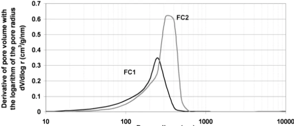
In this part, the model is tested to study the behaviour of fired clay materials subjected to frost analysed in experimentations presented in [24]. In this experimental campaign, the behaviour of fired clay materials with different physical and mechanical properties (porosity, permeability, mechanical strength and elasticity modulus) was subjected to freeze–thaw cycles (temperature lying between 15°C and -16°C) [24]. Density, porosity and pore size distribution, permeability, Young modulus and tensile strength of the two materials (Table 1 and Figure 2) were measured [24]. The specimens subjected to freeze–thaw cycles were prismatic (length = 170 mm, width = 115 mm, thickness = 19 mm – Figure 3). The two porous materials present different frost behaviours: the first one, FC1, is quickly damaged (the first cracks appeared before 15 cycles) while FC2 shows a high resistance to frost action (cracking occurred after 135 cycles) [24]. The differences of behaviour can be explained by permeability (Table 1 - FC2 is more permeable than FC1), mechanical properties (Table 1) or by the difference in pore distribution (Figure 2). Moreover, the temperature and the strains of the specimens during the cycles were measured (the places of the sensors are shown in Figure 3). The coefficient m of van Genuchten’s relation (Equation 31) was determined for two porous materials close to those studied in this paper [25, 26]. The mean value of the two measurements (m = 0.5) was kept for the calculations carried out in this analysis. A study of sensitivity to this parameter is also performed below.

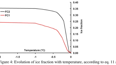
In fired clay, the water in the pores is poor in ionic species. This is one of the advantages of testing the model on this type of materials because ionic species modify the melting temperature of water, which makes the problem more complex [16]. In this paper, the effect of the pore size distribution on the frost durability of porous materials [1-9] is taken into account by the progressive development of the ice in the pores (Equations 7 and 11) and by the action of the ice on the pore walls (Equation 18). In order to solve these equations, the pore size distributions of the two porous media are needed (Figure 2). Figure 4 shows the development of the ice according to the temperature in the porosity (using equation 11). This figure does not represent a state of the material at a given time but shows an intrinsic relation between the temperature and the ice fraction in the material taking into account the pore size distribution. If the temperature is known in a point of the specimen, the relation presented in Figure 4 gives the ice fraction in this point. The ice fraction in material FC2 is greater than in FC1 due to the higher porosity. Moreover, the pores with radii larger than 60 nm are filled by ice crystals at -1°C (Equation 7). Thus the porosity of the two materials is almost full of ice once the temperature reaches -1°C (Figure 4).

The numerical problems are analysed on these two materials. Thermal calculations were carried out in 3D analyses. The poromechanical calculations can be very long because of the high variation rate of the equation coefficients. The problem is particularly time consuming

for 2D and 3D analyses. Therefore, mechanical calculations were performed in one- and two-dimensional analysis and discussed with respect to experimental measurements.

5.2 Parameters

The constants concerning liquid water and ice, which are necessary to perform the thermal and the mechanical calculations, have been taken from [15, 16, 19] (Table 2). In order to determine the pore radius above which the porosity is filled by ice (Equation 7), the melting entropy ΣM was taken constant and equal to 1.2 MPa/K given by [13, 14]. The thermal

calculations need the enthalpy of fusion of ice per unit of mass L_l>i, which depends on the temperature and can be deduced from [27]:

(

)

3

(

)

2 3 5 10 0125 . 0 10 83 . 4 10 34 . 3 _{m m} i l T T T T L_> = × − + × − − + × − − (40)

The mechanical calculations require the surface tension between liquid water and ice γ_li

( )

T to be quantified (Equation 17) [15]:

(

)

(

₃₆+_0.25 −

)

×₁₀−3 = m li T T γ (41)

in N/m, and the evolution of the liquid water viscosity with the temperature [28]:

( )

₍

_{) (}

_{) (}

₎

_       + + + + + = ₃ 0 3 2 0 2 0 1 0exp t T B t T B t T B T l η η (42)

with η0 = 4.601x10-5 mPa.s, B1 = 3068.6°C, B2 = -3.3775x105°C2, B3 = 1.4781x107°C3 and t0

= 123.15°C.

5.3 Thermal calculations

5.3.1 Specimen geometry and meshes

As the specimens have three planes of symmetry (Figure 3), only an eighth of them have to be meshed if a realistic representation of the edge effect is sought. Of course, in this case, the heat flux is taken to be 0 on the planes of symmetry of the problem. The direction and the cross-section studied in 1D and 2D analysis respectively are defined in Figure 3.

5.3.2 Boundary conditions and objectivity

Before freezing, the specimens were subjected to progressive soaking in water during the time necessary to saturate the whole porosity. Then, the water was removed and the specimens kept in air at 15°C. The temperature of the air was reduced rapidly to reach -5°C after 15 min. and -16°C after 2 hours [24]. In this paper, only the negative temperature have been analysed (Figure 5). During freezing, they were exposed to air on the six faces. The air temperature Tair

was given by measurement [24] and the boundary condition was a heat flux related to this imposed temperature:

(

T T

)

n

h − _air

=

ϕ (43)

with ϕ the heat flux, h the heat transfer coefficient, Tair the temperature of the air surrounding

No objectivity problems with mesh size were observed during the thermal calculations. However, some problems of convergence appeared for large time steps. In order to perform the thermal calculations, a method analogous to that presented just above for the pressure calculations (Eq 39) was used (with a limit of temperature variation, ∆Tlim, of 0.1°C). The

heat transfer coefficient h was determined by curve fitting so that the temperature calculated at the position of the temperature sensor was equal to the measured temperature (Figure 5).

5.3.3 Comparison between calculations and experiments

The temperature measurement at the location of the sensor (Figure 3) is well reproduced for the two materials (Figure 5). Without the sink term due to this latent heat, the thermal behaviour of the specimens appears to be very different, with temperature always close to the air temperature (Figure 5). Due to the latent heat created by the ice formation, the specimens’ temperature stays quite constant and close to 0°C over a long period and decreases later than without ice formation.

However, the fitting of the temperature measurement of FC1 is obtained for a heat transfer coefficient of 26 W/m2_{/K while the coefficient is equal to 34 W/m}2_{/K for the second material.}

The first value is quite usual for transfer in a well ventilated environment as in the tests studied here. However, it is quite unusual to obtain coefficients that are so different for specimens in a similar environment. If the calculation of FC2 is performed with the coefficient obtained for FC1, the calculated temperature decreases less rapidly than the temperature measured on the real specimen (Figure 5).

Different thermal behaviour between FC1 and FC2 could be expected because of the differences of water porosity (Table 1). Material FC2 has considerably greater porosity than material FC1 (37% versus 25%). If the porosity is saturated by water, the volume of ice created in the specimens should be greater in FC2 than in FC1 with a difference of about 30% as shown in Figure 2. Thus, more latent heat should be created when the temperature of the FC2 specimen falls to below 0°C and the decrease of temperature in FC2 should be slower than for FC1 as already observed in previous experiments in the same conditions on comparable materials [25]. Therefore, the thermal calculations show possible problems during the experimentation: either the specimens were not in exactly the same conditions (heat transfer coefficient different for the two materials) or the FC2 specimens were not totally saturated. However, the physical mechanisms are complex and assumptions made to perform the calculations (constant heat transfer coefficient, kinetics of the transformation of liquid water in ice…) could lead to approximations in the results.

5.3.4 Comparison between 1D, 2D and 3D calculations

The evolution of temperature at characteristic points of the specimens obtained in 1D, 2D and 3D calculations have been plotted in Figure 7 in order to assess the impact of the different assumptions on the thermal results. In the comparison between 1D and 3D, two points have been defined: point P1 is the core of the specimen and P5 is the centre of the external surface (Figure 6). Because the specimens are flat plates, the boundary conditions have little effect on the temperature in the centre (Figure 6). This result is confirmed by the comparison of the thermal evolution at the two points P1 and P5 (comparison between 1D and 3D analyses) and at the position of the temperature sensor (comparison between 2D and 3D analyses) obtained by the three analyses (Figure 7). Therefore, the 1D and 2D analyses used to investigate the behaviour of the fired clay under frost action have little effect on the thermal results at the characteristic points of the study.

5.4 Mechanical calculations

5.4.1 Boundary conditions

Usually, authors assume that the surface of the specimens is covered by a thin ice layer [19] and that the interface between the ice crystal and the external air is flat as proposed in [5]. The ice is then subjected to atmospheric pressure [16, 19]. Equation 44 then gives the boundary conditions for the liquid pressure:

( )

( )

_{( )}

( )

T R T T T p eq li l γ κ =−2 − = (44)

Equation 7 gives the expression for Req(T) and equation 44 becomes:

( )

T

(

T T

)

p_l =−Σ_{M m} − (45)

T is negative temperature; thus it leads to suction on the boundary.

5.4.2 Calculation objectivity

Time-step influence

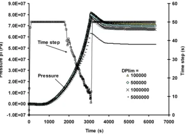
The mechanical problem of frost development in porous media presented above is highly non-linear due to the non-non-linearity of the coefficients in equations 34 and 35. This non-non-linearity, from a physical point of view, corresponds to the propagation of the ice front in the specimen (Figure 8 for 1D calculation on FC1). Therefore, it is important to give careful consideration to the problem of objectivity according to time-step and mesh size. The time-step control proposed above (Equation 39) is presented for 1D calculations and its effect is analysed on the value of the pressure in the core of the FC1 specimens (point P1 – Figure 9). If the limit pressure increment ∆Plim is too large (greater than 1 MPa for FC1 and FC2), the calculations

appear to be non-objective (Figure 9). For smaller values, the different calculations give similar results. The value of 1 MPa was used for all the following calculations. This value depends on the type of porous medium and particularly on the pore size distribution and has to be determined for each material. Figure 9 shows the performance of the time control proposed with the representation of the time steps necessary to perform objective calculations. When the pressure variations are small (at the beginning and at the end of the calculation), the time step is maximal (equal to 50 seconds in this paper). As soon as the pressure variations become large, the time step decreases to reach values of less than 10 seconds for a 1D calculation (it can reach less than one millisecond for 2D and 3D calculations as discussed below). Thus, the time step is always in good accordance with the pressure evolution in the specimen. The calculation is performed with long time steps when there is no evolution and short time steps when the evolution is rapid.

Influence of mesh element size

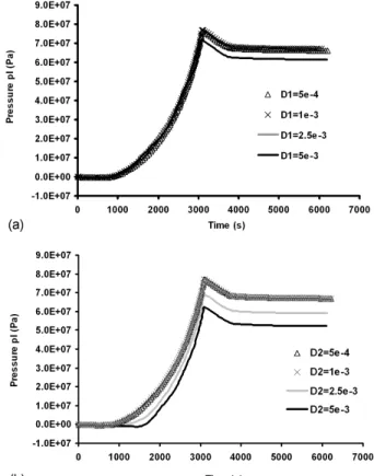
In order to investigate the objectivity according to mesh size, calculations with various densities of the mesh in the core of the specimen (density D1) and near the external surface (density D2) were performed with 1D calculation. When one of the two densities varied, the other was taken to be equal to 1 mm. The dependence of the pressure in the core of the specimen (point P1) on mesh size is represented in Figure 10 for material FC1. The mesh size in the core of the specimen mainly has an impact on the maximal pressure but the impact on the kinetics is small (Figure 10a). In contrast, the mesh density close to the external surface

has an effect on the kinetics and on the maximal pressure (Figure 10b). In fact, the effect on the kinetics is mainly a delay in the increase of pressure at the beginning of the test (around 1000 and 2000 seconds) which is never compensated and explains the difference of maximal pressure. This delay is due to the development of ice crystals in the specimen. The increase of the pressure in the specimen is explained by the term S of equations 27 and 28 and by the decrease in the permeability. The larger the first element is, the longer is the time to reach a temperature cold enough to close the porosity and thus to decrease the permeability sufficiently. For the two materials, a constant density of 1 mm in the whole specimen appears to be necessary to obtain precise calculations.

5.4.3 Comparison between calculations and experiments

Once the problem of objectivity had been treated, calculations were carried out in order to compare the calculated strains with the measurements performed during the experiment [24]. 1D calculation is not sufficient to compare computed and experimental values because of the position of the strain gauge on an edge of the specimen (and not in the middle where the 1D calculation is performed, see Figure 3), so 2D or 3D analyses are necessary. However, in 2D and 3D calculations, the evolution of the pressure can be rapid particularly at singular points like corners. The time control method proposed above then leads to time steps tending towards zero and thus the calculations become impossible. The 3D calculations could only be performed on the first 800 seconds (while the duration of the experiment was about 6500 seconds), which did not allow interesting comparisons to be made with experiment. 2D calculations could be performed over a longer time (about 2000 s) and were used for this analysis.

Figure 11 presents the initial and the deformed specimens at 2000 s for material FC1. At this time step, the deformation according to the height (direction z in Figure 11) is smaller on the small external face (point P4) than in the core of the specimens (point P1). Figure 12 shows that the difference begins to appear at about 1500 s. Before 1500 s, the porosity at the external boundary is not completely filled by ice and the permeability is still quite large. Thus the pressure in the specimens is quite uniform and so are the deformations. After 1500 s, the permeability decreases rapidly and first on the external boundary. The external points are then subjected to negative liquid pressure (Equation 42) while the liquid pressure in the core of the specimen increases due to ice formation and low permeability, causing the divergence of behaviour. This result is in accordance with the experimental observations which show the largest damage in the central part of the specimens [24]. The gradient of strains induced in the specimens leads to tensile stresses close to the external surfaces in the two directions, along the length y and the height z, and to smaller total stresses in the core.

The deformed specimens determined by calculations are in accordance with the experimental observations. However, the calculated strains appear to be too large compared to the measurements. The two materials showed the same strain through the height of the specimens during cooling (Figure 13). In order to compare the calculated value with the measurement, the calculated strain was determined as the average of the strain at point P4 and at a point located 5 mm above in order to take the length of the gauge sensor into account. For FC1, the calculated value is positive, as expected and observed in Figure 11 while, for FC2, the calculated value is negative (Figure 13). The analysis of the pressure in the core of the specimens (Figure 14) shows that the problem of time objectivity is more important in 2D calculations than in 1D. For material FC1, the pressures in the core of the specimen in 1D and 2D calculations are equal, as expected due to the large width and length of the specimens compared to their height (Figure 14). For material FC2, the calculated pressures obtained for the two calculations are totally different, which can be explained by the objectivity problem.

The problem of objectivity is more severe for FC2 due to faster ice development (Figure 4) and larger porosity of the material, which cause faster and larger pressure increase and thus higher non-linearity. Thus, materials with large porosity and quite uniform pore radius give highly non-linear calculations and are difficult to analyse with 2D calculations.

Figure 13 shows that the value calculated for the FC1 specimen is about 10 times larger than the measurements. Therefore, with realistic input data, the calculation results are unrealistic. This can be explained by experimental problems, like crack development around the strain gauge or by unrealistic assumptions made in the development of the model. Thus, it could be interesting to perform measurements to determine the ice development according to the temperature on these two porous materials [25, 26, 29] in order to compare the usual relation between ice crystal radius and temperature (Equation 7) with experimentation. Another assumption is to assess the decrease of permeability with ice development using van Genuchten’s relation (Equation 31). This relation represents the reduction of the permeability with the decrease of the liquid fraction in the porosity and was initially established by Van Genuchten for unsaturated soils where the two phases were water and air [22]. The initial Van Genuchten’s relation has already been modified for gas permeability in order to better describe the measurements in cement based materials [30]. Therefore, the decrease of water permeability with ice development by van Genuchten’s relation may not be representative of reality. In order to study the effect of this relation on the calculated strains, the calculations were performed with coefficient m (Equation 31) varying from 0.5 (the initial value) to 1 (Figure 15). With larger coefficients, the decrease of the permeability with decreasing temperature is slower: for a given temperature, the permeability is higher for m equal to 1 than for m equal to 0.5. With higher permeability, the liquid pressure is lower and thus the resulting strains are smaller as shown in Figure 15. The strains obtained with m lying between 0.8 and 1 are close to the measured strains during the 2500 first seconds. However, after this time, the liquid pressure is mainly driven by the negative pressure at the boundary. Thus, after 2500 seconds, the pressure and the strains decrease while the measured strain does not show any decrease and remains at constant values.

5.4.4 Comparison of the two materials

The finite element poroelasticity formulation presented in this paper takes account of the main thermal and poromechanical parameters involved during ice development in porous media and their coupled effects. Although the previous comparison with experiment shows that the model overestimates the frost consequences, it can be used to compare the behaviour of porous media subjected to frost action from usual material parameters. In this part, the behaviour of the two materials, FC1 and FC2, under frost conditions is calculated with 1D analysis in order to analyse the differences that could explain the high frost resistance of FC2 and the low frost resistance of FC1. The comparison is made in terms of pressure (determined in the core of the specimen – point P1 – Figure 16a) and total stress along the length (determined in the core and on the external surfaces – points P1 and P5 – Figure 16b). The pressure is about twice as great in material FC2 as in FC1 (Figure 16a). This can be explained by:

- the greater porosity: the greater the porosity, the larger the pressure increase due to the volume increase during the transformation of liquid water in ice. This is already observed in some empirical models used to assess the frost resistance of fired clay [7]. - the higher Young’s modulus: the greater the Young’s modulus, the larger the pressure

increase. This is usually not considered in the empirical models, which focus on the size pore distributions without taking the mechanical properties into consideration [24] The effects of these two parameters on the pressures could have been diminished by the greater permeability of FC2. Greater permeability implies that a larger quantity of liquid

water can go out of the porous media without increasing the pressure. However, van Genuchten’s relation (Equation 31) causes a fast decrease of the permeability with liquid saturation and thus with temperature. Therefore, the permeability of the two materials is quickly of the same order, particularly close to the boundary.

The total stresses are negative (compressive stresses) in the core of the specimens and positive close to the boundary (tensile stresses). The total stresses are due to the gradient of strains induced by the ice formation and vary according to the propagation of the ice front. The tensile stresses are of the same order for both materials while the compressive stresses are greater for FC2. However, they are small (lower than 3 MPa) compared to the effective stresses due to the pressure term (Equation 23). With the mechanical characteristics of the material given in Table 1, the Biot coefficients are about 0.59 for FC1 and 0.75 for FC2. Therefore, the effective stresses are mainly negative close to the boundary, due to the negative imposed liquid pressure at the boundary (Equation 45 – Figure 16b), and are positive in the core of the specimens (due to positive pressure – Figure 16b). In the core of the specimens, the tensile effective stresses reach about 40 MPa for FC1 and 140 MPa for FC2. These stress values are positive and can explain the damage observed during frost experiments. However, they are largely greater than the tensile strength of the material (Table 1), while FC2 presents high frost durability with no major cracking before 135 cycles [24]. It confirms the overestimation of the frost effect on porous media already pointed out by the comparison of the calculated and measured strains.

Therefore, the comparison of the behaviour of the two materials based on the coupled effects of the physical and mechanical properties during frost action does not explain the differences of behaviour of the two fired clays (poor resistance for FC1 and high resistance for FC2). However, the thermal calculations show that the FC2 specimens could not have been totally saturated. This lack of saturation could then explain the better frost resistance during the test. Supplementary experiments on materials with good frost resistance appear to be necessary to test again the capability of the model to assess the behaviour of porous media to frost.

6. Conclusion

Assessing the effect of ice development in porous media is a complex problem. The framework of poromechanics [17] can be used to evaluate the consequences of ice development in porous media in terms of pressure, strains and stresses. The aim of the paper was to present the comparison of the calculations based on an existing model [15] using the finite element formulation with experimentation performed on fired clays. In the approach presented here, the thermal and the mechanical problems have been considered as uncoupled. The thermal problem does not pose any difficulties. The latent heat due to ice formation has been successfully taken into account in the usual thermal finite element formulations. The thermal analysis of the two materials has revealed experimental problems (problems of exposure to air or saturation of the porosity). The particularities of the frost model developed by Zuber [15] have been taken into account in the usual finite element poroelasticity formulation. This part of the calculations is highly non-linear, and particular care is required to perform objective calculations. A method to determine the time between two calculation steps according to the evolution of the pressure in the specimen is proposed to avoid over-long calculations and ensure objectivity. Due to the high non-linearity of the calculations, 2D and 3D calculations are difficult for materials with large porosity and narrow pore size distribution. For such analyses, the time steps should be lower than a millisecond to guarantee objectivity. For materials with larger pore size distributions, the ice development would be more progressive, which could slow down the pressure increase and avoid the convergence problem observed for the two materials studied in this paper. The characteristic of the model presented here is to take into account the main thermal and poromechanical properties

involved during ice development in porous media and their coupled effects. This paper is an attempt to validate this model by comparing the calculations with experiments performed on real building materials. The model appears to overestimate the strains and the stresses due to frost action. This can be observed in the large increase of the liquid pressure in the specimen with the ice development and can be explained by the determination of the permeability. The problem of assessing permeability is multiple. First, all the calculations are based on the pore size distribution in accordance with the experimental and theoretical observations of ice mechanisms. However, the pore size distribution was determined by the usual mercury intrusion, which is known to measure the diameter of the pore access and not really the mean pore diameter. Thus the largest pores, which have a great effect on permeability, are neglected by this method. Secondly, the decrease of the permeability with the ice development is determined by van Genuchten’s relation. The paper shows that modifying the parameter of this relation can have an important impact on the results. Finally, the permeability could be greater than assumed due to the development of micro cracking in the material. Such micro cracking could be caused by the large tensile effective stresses and imply an increase of the permeability as early as the first cooling. This phenomenon could be taken into account using damage modelling of the material matrix. Furthermore, new experiments appear to be necessary to study, in particular, the evolution of permeability with ice development in porous media.

Acknowledgement

The authors acknowledge the Technical Centre for Natural Building Materials (Centre Technique des Matériaux Naturels de Construction – CTMNC) for supporting this work. The authors are also grateful to CEA/DEN/DM2S/SEMT for providing the finite element code CASTEM2000.

References

1. Powers TC. The air requirement of frost-resistant concrete. Proc. Highway Res. Board, PCA Bulletin 33, Portland Cement Association, Skokie, 1949; 29 : 184-211. 2. Powers TC, Helmuth RA. Theory of volume changes in hardened Portland cement

paste during freezing. Proc. Highway Res. Board, PCA Bulletin 33, Portland Cement Association, Skokie, 1953; 32 : 285-297.

3. Litvan GG. Phase transitions of adsorbates: Part IV. Mechanisms of frost action in hardened cement paste, Journal American Ceramic Society 1972; 55 : 38-42.

4. Cheng-yi H, Feldman RF. Dependence of frost resistance on the pore structure of mortar containing silica fume. ACI Journal Proceedings 1985; 82 : 740-743.

5. Setzer MJ. A new approach to describe frost action in hardened cement paste and concrete. Proceedings of the conference on hydraulic cement paste, British Cement and Concrete Association, Sheffield, England, UK, 1976; 312-325.

6. Ravaglioli A. Evaluation of frost resistance of pressed ceramic products based on the dimensional distribution of pores. Transaction of the British Ceramic Society 1976; 76 : 92-95.

7. Maage M. Frost resistance and pore size distribution in bricks, Materials and Structures 1984; 17 : 345-350.

8. Robinson GC. The relation between pore structure and durability of bricks. Ceramic Bulletin 1984; 63 : 295-300.

9. Hansen W, Kung JH. Pore structure and frost durability of clay bricks. Materials and Structures 1988; 21 : 443-447.

10. Penttala V. Freezing - Induced strains and pressures in wet porous materials and especially in concrete mortars. Advanced Cement Based Materials 1998; 7 : 8-19. 11. Scherer GW. Freezing gels. Journal of Non-Cryst Solids, 1993; 155 : 1-25.

12. Scherer GW. Crystallization in pores. Cement and Concrete Research 1999; 29 : 1347-1358.

13. Coussy O, Monteiro PJM. Poroelastic model for concrete exposed to freezing temperatures. Cement and Concrete Research 2008; 38 : 40-48.

14. Coussy O. Poromechanics of freezing materials. Journal of Mechanics and Physics of Solids. 2005 ; 53 : 1689-1718.

15. Zuber B, Marchand J. Modeling the deterioration of hydrated cement systems exposed to frost action Part 1: Description of the mathematical model. Cement and Concrete Research 2000; 30 :1929-1939.

16. Zuber B, Marchand J. Predicting the volume instability of hydrated cement systems upon freezing using poro-mechanics and local phase equilibria. Materials and Structures 2004; 37 : 257-270.

17. Coussy O. Poromechanics. Wiley: New York, 2004.

18. Bazant ZP, Chern J., Rosenberg AM. Mathematical model for freeze-thaw durability of concrete, Journal American Ceramic Society 1988; 71 : 776-783.

19. Boukpeti N. One-dimensional analysis of a poroelastic medium during freezing. International Journal forNumerical and Analytical Methods in Geomechanics 2008;

32 : 1661-1691.

20. Fagerlund G. Determination of pore-size distribution from freezing–point depression. Materials and Structures 1973; 6 : 215-225.

21. Biot MA. General theory of three-dimensional consolidation. Journal of Applied Physics 1941; 12 : 55-164.

22. van Genuchten MTh. A closed-form equation for predicting the hydraulic conductivity of unsaturated soils. Soil Science Society American Journal 1980; 44 : 892-989. 23. http://www-cast3m.cea.fr/cast3m/html/ManuelCastemEnsta/node4.html

24. Perrin B, Vu NA, Multon S, Voland T, Ducroquetz C. Mechanical behaviour of fired clay materials subjected to freeze–thaw cycles. Construction and Building Material 2010, doi:10.1016/j.conbuildmat.2010.06.072.

25. Wardeh G. Les phénomènes de gel-dégel dans les matériaux à base de terre cuite et les conséquences sur leur durabilité. Expériences et modélisation. PhD thesis, Toulouse University, France, 2005.

26. Wardeh G, Perrin B. Freezing-thawing phenomena in fired clay materials and consequences on their durability. Construction and Building Material 2008; 22 : 820-828.

27. Matala S. Effects of carbonation on the pore structure of granulated blast furnace slag concrete. 1995, Helsinki University of Technology, Faculty of the Civil Engineering and Surveying Concrete Technology, Espoo, Finland.

28. Grant SA. Physical and chemical factors affecting contaminant hydrology in cold environment. Technical TR-00-21, U.S. Army Corps of Engineers, ERDC/CRREC, 2000.

29. Wardeh G, Perrin B. Numerical modelling of the behaviour of consolidated porous media exposed to frost action. Construction and Building Material 2008; 22 : 600-608.

30. Monlouis-Bonnaire JP, Verdier J, Perrin B. Prediction of the relative permeability to gas flow of cement-based materials. Cement and Concrete Research 2004; 34 : 737-744

Tables

Table 1: Input data for two porous materials (fired clays) [24]

Parameter Symbol Identification FC1 FC2 Units

Physical properties

Density ρs measurement 1900 1700 kg/m3

Porosity n measurement 0.25 0.37

Permeability D measurement 4.0x10-17 _1.5x10-16 _m2

Thermal properties

Conductivity λs usual value 0.5 0.5 W/m/K

Heat capacity cs usual value 900 900 J/kg/K

Mechanical properties

Volumetric thermal dilation αs usual value 20x10-6 20x10-6 K-1

Young modulus E0 measurement 3.85 9.90 GPa

Poisson coefficient ν₀ usual value 0.2 0.2

Tensile strength ft measurement 1.1 2.7 MPa

Table 2: Input data for liquid water and ice [15, 16, 19]

Parameter Symbol Liquid water Ice Units

Physical properties

Density ρl, ρi 1000 920 kg/m3

Thermal properties

Conductivity λl, λi 0.57 2.20 W/m/K

Heat capacity cl, ci 2100 4220 J/kg/K

Melting entropy ΣM 1.2 MPa/K

Mechanical properties

Volumetric thermal dilation αl, αi

(

−9.2+2.07∆T

)

.10−5

5 10 . 200 1 5 . 16  −      ∆ + T K-1

Figures

Figure 1: Development of ice crystal in the porous media according to the pore size

Figure 2: Pore size distribution of the two porous materials obtained by Mercury Intrusion Process

Figure 3: Specimens (P1 is at the core of the specimen, P5 is the centre of the external surface of the specimen) and measurement equipment

Figure 4: Evolution of ice fraction with temperature, according to eq. 11 and pore size distribution supplied in Figure 2

Figure 5: Evolution of the temperature at the temperature sensor level for the two materials (the air temperature is the measurement performed by the sensor shown in Figure 3)

Figure 6: Temperature in the FC1 specimen at 1000 s (a), 2500 s (b) and 4000 s (c)

Figure 7: Calculated temperatures at the sensor position and at the centre of the specimen in 3D, 2D and 1D calculations (for the points P1 and P5 see Figures 3 and 6)

Figure 8: Propagation of the ice front in the depth of the FC1 specimen in 1D calculation

Figure 9: Analysis of the time objectivity according to the limit pressure increment ∆Plim for FC1 and evolution of the time steps obtained for ∆Plim = 1 MPa in 1D calculation

Figure 10: Analysis of the objectivity according to the mesh size on the total kinetics for FC1 for various densities in the core of the specimen D1 (a) and close to the external surface D2 (b)

Figure 11: Initial (red contour) and deformed meshes of FC1 specimen after 2000 seconds (2D calculation)

Figure 12: Calculated strains in the z direction (specimen height direction) in the core (P1) and on the external surface (P4) for 2D calculation

Figure 13: Measured and calculated strains in the z direction (specimen height direction)

Figure 15: Effect of the decrease of the permeability with ice development on the calculated strain (m is the Van Genuchten exponent)

Figure 16: Pressure evolution at P1 (a) and stress evolution at P1 and P5 (b) versus time for FC1 and FC2 specimens (1D analysis) (for the points P1 and P5 see Figures 3 and 11)