HAL Id: hal-01137935
https://hal.archives-ouvertes.fr/hal-01137935
Submitted on 3 Apr 2015
HAL is a multi-disciplinary open access
archive for the deposit and dissemination of
sci-entific research documents, whether they are
pub-lished or not. The documents may come from
L’archive ouverte pluridisciplinaire HAL, est
destinée au dépôt et à la diffusion de documents
scientifiques de niveau recherche, publiés ou non,
émanant des établissements d’enseignement et de
Reaping the carbon rent: Abatement and overallocation
profits in the European cement industry, insights from
an LMDI decomposition analysis
Frédéric Branger, Philippe Quirion
To cite this version:
Frédéric Branger, Philippe Quirion. Reaping the carbon rent: Abatement and overallocation profits
in the European cement industry, insights from an LMDI decomposition analysis. Energy Economics,
Elsevier, 2014, 47, pp.189-205. �10.1016/j.eneco.2014.11.008�. �hal-01137935�
Reaping the carbon rent: abatement and overallocation
profits in the European cement industry, insights from
an LMDI decomposition analysis
— Pre-Print —
Frédéric Brangera,b,1,∗, Philippe Quiriona,c
aCIRED, 45 bis, avenue de la Belle Gabrielle, 94736 Nogent-sur-Marne Cedex, France bAgroParistech ENGREF, 19 avenue du Maine 75732 Paris Cédex
cCNRS, France
Abstract
We analyse variations of carbon emissions in the European cement industry from 1990 to 2012, at the European level (EU 27), and at the national level for six major producers (Germany, France, Spain, United Kingdom, Italy and Poland). We apply a Log-Mean Divisia Index (LMDI) method, cross-referencing data from three databases: the Getting the Numbers Right (GNR) database devel-oped by the Cement Sustainability Initiative, the European Union Transaction Log (EUTL), and the Eurostat International Trade database.
Our decomposition method allows seven channels of emissions change to be distinguished: activity, clinker trade, clinker share, alternative fuels, thermal and electrical energy efficiency, and electricity decarbonisation. We find that, apart from a slow trend of emissions reductions coming from technological im-provements (first from a decrease in the clinker share, then from an increase in alternative fuels), most of the emissions changes can be attributed to the activity effect.
Using counterfactual scenarios, we estimate that the introduction of the EU ETS brought small but positive technological abatement (2.2% ± 1.3% between 2005 and 2012). Moreover, we find that the European cement industry has gained 3.5 billion Euros of “overallocation profits”, mostly due to the slowdown of production.
Key-words
Cement Industry, LMDI, EU ETS, Abatement, Overallocation, Windfall Profits, Overallocation Profits, Carbon Emissions, Energy Efficiency
∗Corresponding author
Email addresses: branger@centre-cired.fr (Frédéric Branger),
1. Introduction
Cement is the most widely-used man-made material in the world (Moya et al., 2010), and also one of the most carbon-intensive products. The manufac-ture of cement accounts for approximately 5% of global anthropogenic emissions (IEA, 2009). China has the lion’s share of cement production with 58% of the 3,700 million tons produced in 2012. The European Union is now the third-biggest producer with 5% of global production, behind India with 7% (U.S. Geological Survey, 2013).
Since 2005 European cement emissions have been covered by the European Union Emission Trading Scheme (EU ETS), presented as Europe’s flagship pol-icy to tackle climate change (Branger et al., 2013a). In this cap-and-trade sys-tem, installations can buy or sell tradable allowances to attain emissions caps. A key feature of the EU ETS, the question of whether allowances should be auctioned or received free of charge (and in the latter case, what should be the allocation plan, or the number of allowances per installation), has proved to be a very controversial topic (Boemare and Quirion, 2002; Ellerman and Buchner, 2007). While most economists favored auctioning, the European Union opted for almost completely free allocation for all sectors (industry and power sector) during phase I (2005-2007) and phase II (2008-2012); and maintained completely free (but declining at 1.74% per year) allocations1 in phase III (2013-2020) for
sectors “deemed to be exposed to carbon leakage”, and partly free for the rest of manufacturing industry (European Commission, 2009).
Indeed, the main argument used to justify free allocation has been the preservation of heavy industries’ competitiveness and the prevention of car-bon leakage, which is a shift of emissions from carcar-bon-constraint countries to less carbon-constrained countries induced by asymmetric carbon pricing (Dröge, 2009). However, economic theory suggests that free allocation, if independent from current production, is inefficient at preventing leakage in the short term and would only provide a disincentive to plant relocation (Wooders et al., 2009). In other words, in the short run free allocations would compensate firms for profitability losses without addressing market share losses and carbon leakage (Cook, 2011).
In addition to generous allocation caps, the economic downturn after 2008 led to a decrease in industrial production, which generated a large surplus of allowances in the market. These financial assets have mainly been held by cement and steel companies, because electricity demand has been much less
1Allocations in phase III are based on a product benchmark (the average of the 10% best
performing installations: 766kg CO2 per ton of clinker, the CO2-intensive intermediate prod-uct required to produce cement), multiplied by a “cross sectoral correction factor” (0.9422 in 2013, declining by 1.74% per year), historical activity level (HAL, a formula leading approx-imately to pre-crisis level of production), and an “activity level correction factor” (reducing allocations by half or four if the plant is functioning below 50% or 25% of its HAL). Completely free allocations are then maintained though the overall cap of allowances is less generous (it has been reduced by 23% between 2012 and 2013) and declining. However because actual production is much lower than pre-crisis level, 2013 emissions were 20% lower than the cap.
impacted by the economic downturn.
Instead of suffering from financial losses, energy-intensive industries seem to have thrived from the scheme. Sandbag, a non-governmental organization, has estimated that the ten “carbon fat cats” have reaped billions of Euros in windfall profits (Pearson, 2010). However, their analysis, based on the European Union Transaction Log (EUTL) data, is based upon equivalence between allowances surplus and overallocation, without considering the fact that some allowances are obtained by reducing the carbon content of industrial products (Ellerman and Buchner, 2008). Indeed, apart from financial outcomes, an important ques-tion remains: whether the EU ETS has fulfilled its original purpose which was to trigger a transition towards low-carbon industry.
Studies assessing abatement in the manufacturing industry have obtained mixed results (Neuhoff et al., 2014). Zachman et al. (2011) find a significant reduction in carbon intensity for basic metals (whose emissions occur mostly in the steel sector) and non-metallic minerals (whose emissions occur mostly in the cement sector) between 2007 and 2008 compared to 2005-2006. Yet (Kettner et al., 2014) find very limited reduction in carbon intensity in the cement and lime sector, and attribute most of it to an increase in clinker imports – which implies carbon leakage. Moreover Egenhofer et al. (2011) find almost no decrease in the manufacturing industry’s carbon intensity in 2008, which seems to contradict Zachman et al. (2011) results.
In this paper, we propose to shed light on the questions of abatement and overallocation in the European cement industry, exploiting EUTL data, Eu-rostat international trade data, and the detailed and comprehensive Getting the Numbers Right (GNR) database from the Cement Sustainability Initiative (CSI). We perform an LMDI (Log Mean Divisia Index) decomposition (Ang, 2004) of emissions due to cement production in Europe. We measure the impact of seven effects on emissions variations, which correspond to different mitiga-tion levers: activity, clinker trade, clinker share, alternative fuel use, thermal and electrical energy efficiency, and decarbonisation of electricity. This analysis allows us to identify the key drivers behind changes in aggregated carbon emis-sions, in the EU 27 as a whole and in six major European producers: Germany, France, Spain, the UK, Italy and Poland.
A distinction can be made between the first two effects (activity and clinker trade) that generate non-technological abatement and the others that generate technological abatement. Making assumptions on counterfactual scenarios, we estimate the technological abatement induced by the EU ETS and break down its main factors. Furthermore, our emissions decomposition model allows us to identify which part of the allowances surplus (allocations minus emissions) is due to technological performance and which is due to a change in activity or clinker outsourcing. We are then able to compute overallocation and “overallocation profits”.
We find that the EU ETS has induced a small but positive abatement of 26 Mtons of CO2 (±16 Mtons) from 2005 to 2012 (corresponding to a 2.2% ±
1.3% decrease), mostly thanks to the reduction in the clinker-to-cement ratio. However we cannot rule out another explanation, i.e. the massive increase in
steam coal and petcoke prices in the 2000s (Cembureau, 2012). This aggregate figure hides important differences at national levels. Whereas technological abatement has been important in Germany (5% ± 3%) and in the UK (4% ± 3%), it has been small in France, and insignificant or negative in Spain, Italy and Poland. In addition, we estimate that the European cement industry has reaped 3.5 billion Euros of overallocation profits during phases I and II. Most of these profits come from the economic downturn that has reduced the demand for cement and thus for cement production, in turn generating a massive surplus of allowances.
The rest of the article is structured as follows. Section 2 details the ce-ment manufacturing process and the mitigation options. Section 3 explains the emissions decomposition methodology. Section 4 applies this decomposition to changes in emissions in the European cement industry from 1990 to 2012. Sec-tion 5 is an assessment of technological abatement induced by the EU ETS and of overallocation profits. Section 6 concludes.
2. Mitigation options in the cement industry 2.1. Cement manufacture at a glance
Cement manufacture can be divided into two main steps: clinker manufac-ture, and blending and grinding clinker with other material to produce cement. Clinker is produced by the calcination of limestone in a rotating kiln at 1450 degrees Celsius. Carbon dioxide is emitted in two ways. First, the chemical reaction releases carbon dioxide (ca. 538 kgCO2 per ton of clinker2) which
accounts for roughly two thirds of carbon emissions in clinker manufacture. The remaining CO2 comes from the burning of fossil fuel to heat the kiln. The
fuels used are mostly the cheapest ones, petcoke and coal (the use of gas and oil is precluded by cost, except in some locations where they are very cheap, which is not the case in the EU).
Raw material preparation, kiln operation, blending and grinding consume electricity which causes indirect emissions. However, nearly all carbon emissions (around 95%) in cement manufacture come from direct emissions in clinker manufacture.
To reduce emissions from cement production3, various options are thus avail-able:
2The process CO
2 emission factor is generally considered as a fixed factor. However it is
slightly variable mainly because of the ratio of calcium carbonate and magnesium carbon-ate in the limestone. When process emissions are actually measured, a narrow peak in the distribution can be observed at 538 kgCO2 per ton of clinker (Ecofys et al. (2009) Figure
2). However, the factor used in the EU ETS Monitoring and Reporting of Greenhouse gas emissions (MRG) is only 523 kgCO2 per ton of clinker, derived from IPCC methodology.
3If we consider cement consumption and not cement production, another option can be
added: cement outsourcing. We performed the same analysis for cement consumption with a more complicated decomposition, adding cement trading. As the results barely changed (the cement trading effect represented less than 3 Mtons of CO2or 2% of emissions), for the sake
(i) Reduction of cement production, which may be due to reduced activ-ity in the construction industry, to leaner structures or to the substitution of alternative materials to cement.
(ii) Clinker substitution. Since clinker manufacture is the most carbon inten-sive part of cement manufacture, partially substituting some other material for clinker is an efficient way to reduce emissions per ton of cement produced. The most common type of cement, ordinary Portland cement, is produced by mixing 95% of clinker and 5% of gypsum, but the clinker-to-cement ratio is lowered in blended cements.
(iii) Clinker outsourcing. This is a way to reduce emissions within a given geographical perimeter, but emissions then occur elsewhere, which causes carbon leakage.
(iv) Alternative fuel use, which releases less CO2for the same calorific value
produced.
(v) Energy efficiency, which can be divided into two parts, thermal energy efficiency and electrical energy efficiency.
(vi) Decarbonisation of the electricity. (vii) Carbon capture and storage.
(viii) Innovative cements, or carbon neutral cements based on totally differ-ent processes.
The next section details these options, which do not have the same status. Lever (i) is driven by cement demand and is not a direct choice made by cement companies. Levers (ii) to (v) are operational options used by cement companies (though lever (iii) does not reduce global emissions, it can be a rational choice for a company covered by an emissions trading scheme). Lever (vi) is beyond the scope of cement producers, and depends on electricity producers (which have an incentive to use it when there is a price on carbon). Abatement due to levers (i) to (vi) will be empirically assessed in this study. Levers (vii) and (viii) are in the research and development stage. Though promising, these options have not generated abatement yet.
The challenge of a non-global climate policy is to induce all these options (except (iii)) without generating clinker or cement imports, which would lead to carbon leakage.
2.2. Data sources
The work of this paper is based on the cross-referencing of three databases: • the Getting the Numbers Right (GNR) database4 (WBCSD, 2009)
devel-oped by the Cement Sustainability Initiative (CSI), operating under the World Business Council on Sustainable Development (WBCSD).
4http://wbcsdcement.org/GNR-2011/index.html. Variables have names we will refer to
• the European Union Transaction Log5(EUTL) which is the registry of the
EU ETS, and provides allocations and verified emissions at the installation level.
• the Eurostat international trade database6for clinker trading.
The GNR database covered 94% of European cement production in 2012 (only minor producers with small production volumes are excluded), which is remarkably high. Data are available7 for 1990, 2000, and 2005 to 2012. Data
can be obtained at the EU 28 level and at the national level for big producers (so we have used data for Germany, France, Spain, the UK, Italy and Poland). Although the GNR database contains data on production and emissions, we use this database for its intensity (i.e. rate-based) indicators in the cement industry, for reasons related to coverage and methodology (see part 3.1). A performance indicator not included in GNR, the electricity emission factor, comes from the Enerdata database8.
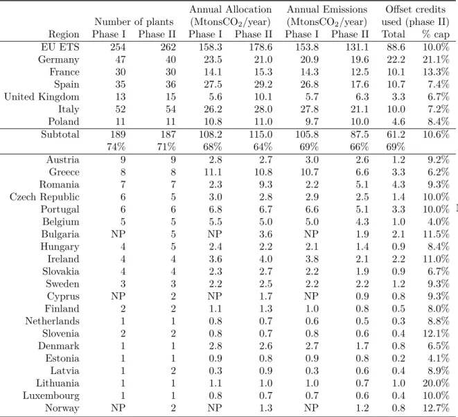
The cement sector is a subsector of the cement/lime EUTL sector (47% of installations and 90% of allocations). We have collected plant-by-plant infor-mation on 276 cement plants with kilns covered by the EU ETS. Some char-acteristics of our cement EUTL database, which are in line with Table 1.2 in European Commission (2010) and Table 4 in Moya et al. (2010)9, are given in Table 1. The match between EUTL emissions and GNR gross direct emissions
5http://ec.europa.eu/environment/ets/napMgt.do
6http://epp.eurostat.ec.europa.eu/newxtweb/setupdimselection.do, EU Trade since 1988
by HS2, 4, 6 and CN8 dataset (extracted in February 2014). The code for clinker is 252310 (“cement clinkers”).
7Due to confidentiality reasons, there is a one year gap between data collection and
publi-cation. The latest data available (2012) were published in August 2014.
8
http://www.enerdata.net/enerdatauk/knowledge/subscriptions/database/energy-market-data-and-co2-emissions-data.php
9Their list contains 268 installations in 2006 at the EU 27 level (compared to 270 for us
(Norway has two cement plants and Croatia four)). There are some discrepancies for France (33 in instead of 30 for us), Germany (38 instead of 43), Italy (59 instead of 52), and some other countries (1 plant difference). In Germany, geolocalization of plants revealed that three plants had two EU ETS installations and 1 had three. Our list was cross-checked with the Cemnet database (http://www.cemnet.com/GCR/), Sandbag database, and public reports of major cement companies.
is good but not perfect10. In addition, we use the Sandbag database11for offset
credits utilization at the installation level.
Whereas total imports and exports are directly available in the Eurostat international trade database at the EU 27 level, they have to be computed from country-pairs raw data at the national level. Also, some corrections needed to be made to take into account the changing geographical perimeter of the EU ETS. Because they are absent from Eurostat, we used the Comtrade database12
for net imports in Norway, Iceland, and the EU 27 before 1999.
2.3. Clinker substitution
Reducing the clinker-to-cement ratio is a very efficient abatement option since most of the carbon emissions are produced during clinker manufactur-ing. The most-used clinker-substituting materials are fly ash (a residue from coal-fired power stations), ground blast furnace slag (a by-product of the steel industry), pozzolana (a volcanic ash) and limestone. Blast furnace cement of-fers the highest potential for clinker reduction with a clinker-to-cement ratio of 5-64%, compared to pozzolanic cement (45-89%) and fly ash cement (65-94%) (Moya et al., 2010).
Two barriers are impeding the deployment of blended cements. The first is the regional availability of the clinker substitutes, or their price (since these products have low value per ton, transportation costs are high). The phasing out of coal-fired plants triggered by climate policy will make fly ash scarcer. Ground blast depends on iron and steel production, and pozzolanas are present only in certain volcanic regions (mainly Italy). Second, the physical proper-ties of these alternative cements such as strength, colour and workability, and their acceptance by construction contractors, constitute another barrier to their implementation (IEA, 2009).
Figure 1 displays the clinker-to-cement ratio in 1990, 2000 and from 2005 to 2012 for the European Union (with 28 member states) and the six biggest cement producers in Europe: Germany, France, Spain, Italy, the United Kingdom and Poland. The average EU 28 clinker-to-cement ratio decreased from 78% in 1990 to 73% in 2012. The UK is the country for which the clinker-to-cement ratio
10GNR emissions are higher in the United Kingdom , Germany and Poland, (3% on
av-erage respectively for all) whereas they are lower Italy and at the EU 27 level (6% and 2% respectively). France and Spain are perfect matches. Besides data-capture errors, differences in emissions can occur for different reasons. First, there is a mismatch in installations covered. GNR contains more plants because it includes grinding or blending plants, but some plants with kilns are not covered, so emissions at the national level have to be extrapolated. Second, accounting methodologies are different. Process emissions are measured in GNR (there is a peak in the distribution at 538 kgCO2per ton of clinker see figure 2 in (Ecofys et al., 2009))
whereas a default factor derived from IPCC methodology of 523 kgCO2 per ton of clinker is
used in the EU ETS. Non-kiln fuels are not reported in some countries for the EU ETS but are (partially) reported in GNR. The carbon content of alternative fuels is also accounted for differently.
11http://www.sandbag.org.uk/data/
Table 1: Cement EUTL database. Country level (Sandbag database used for offset credits)
Annual Allocation Annual Emissions Offset credits Number of plants (MtonsCO2/year) (MtonsCO2/year) used (phase II)
Region Phase I Phase II Phase I Phase II Phase I Phase II Total % cap
EU ETS 254 262 158.3 178.6 153.8 131.1 88.6 10.0% Germany 47 40 23.5 21.0 20.9 19.6 22.2 21.1% France 30 30 14.1 15.3 14.3 12.5 10.1 13.3% Spain 35 36 27.5 29.2 26.8 17.6 10.7 7.4% United Kingdom 13 15 5.6 10.1 5.7 6.3 3.3 6.7% Italy 52 54 26.2 28.0 27.8 21.1 10.0 7.2% Poland 11 11 10.8 11.0 9.7 10.0 4.6 8.4% Subtotal 189 187 108.2 115.0 105.8 87.5 61.2 10.6% 74% 71% 68% 64% 69% 66% 69% Austria 9 9 2.8 2.7 3.0 2.6 1.2 9.2% Greece 8 8 11.1 10.8 10.7 6.6 3.3 6.2% Romania 7 7 2.3 9.3 2.2 5.1 4.3 9.3% Czech Republic 6 5 3.0 2.8 2.9 2.5 1.4 10.0% Portugal 6 6 6.8 6.7 6.6 5.1 3.3 10.0% Belgium 5 5 5.5 5.0 5.0 4.3 1.0 4.0% Bulgaria NP 5 NP 3.6 NP 1.9 2.1 11.5% Hungary 4 5 2.4 2.2 2.1 1.4 0.9 8.4% Ireland 4 4 3.6 4.0 3.8 2.1 2.2 11.0% Slovakia 4 4 2.3 2.7 2.2 1.9 0.9 6.7% Sweden 3 3 2.2 2.5 2.2 2.2 1.2 9.3% Cyprus NP 2 NP 1.7 NP 0.9 0.8 9.3% Finland 2 2 1.1 1.3 1.0 0.8 0.5 8.0% Netherlands 1 1 0.8 0.7 0.6 0.5 0.3 8.8% Slovenia 2 2 0.8 0.7 0.8 0.6 0.4 12.1% Denmark 1 1 2.8 2.6 2.7 1.7 0.8 6.5% Estonia 1 1 0.9 0.8 0.9 0.8 0.2 4.1% Latvia 1 2 0.3 0.9 0.3 0.6 0.4 8.9% Lithuania 1 1 1.1 1.0 1.0 0.7 1.0 20.0% Luxembourg 1 1 0.8 0.7 0.7 0.6 0.4 10.0% Norway NP 2 NP 1.3 NP 1.2 0.8 12.7% Note:
Figure 1: Clinker-to-cement ratio for the EU 28 and main European countries. Source: WBCSD GNR Database, variable 3213
has decreased the most dramatically, from 95% in 1990 to 70% in 2012. In 2012 Germany was the country with the lowest clinker-to-cement ratio, 68%, whereas Spain had the highest, 79%.
2.4. Clinker outsourcing
Clinker outsourcing is a drastic method to reduce carbon emissions within a given geographical perimeter, but it does not in general reduce emissions on a global scale (carbon intensity is approximately the same in Europe and abroad and this adds emissions due to transportation). The increase in emissions abroad due to a regional climate policy is called carbon leakage (Reinaud, 2008). In the EU ETS, free allocation of allowances was presented as a way to mitigate the risk of leakage.
The purpose of this paper is to assess the actual emissions reductions in the cement industry, and not to provide a technology roadmap. Therefore just be-cause clinker outsourcing is an undesirable option does not mean that it should not be considered in this context. Under the EU ETS, it can be profitable since, provided that a certain level of activity is maintained, the operator of an instal-lation keeps receiving free allowances that can be sold on the market. However, logistical difficulties, high transportation costs and export barriers make clinker outsourcing less appealing than it appears. Clinker trading primarily occurs in the case of over- or under-capacity (Cook, 2011). Geography plays an impor-tant role: high road transport costs exclude inland producers from international trade (Ponssard and Walker, 2008).
Figure 2 shows clinker net imports (imports minus exports) divided by clinker production. The EU 27 switched from being a clinker importer to being a clinker exporter in 2009. We can see that clinker is a poorly traded commod-ity: since 1990 net extra-EU27 imports or exports have never been more than
Figure 2: Net imports (imports minus exports) of clinker relative to local clinker production. Sources: Eurostat for net imports, EUTL and WBCSD GNR Database for production
Figure 3: Origin of the EU 27 net imports. West Mediterranean comprises Morocco, Algeria, Tunisia and Libya. Source: Eurostat
7% of its production. Imports came from Asia (mostly China and Thailand) and the East Mediterranean region especially between 2001 and 2005 (mainly Turkey and Egypt), and since 2010 European clinker has mainly been exported to the Gulf of Guinea and Brazil (see Figure 3). The European country with the most remarkable trajectory is Spain, which turned into a massive clinker exporter (20% of its production in 2012) after being a massive importer (up to 34% of its production in 2007). This swing can be explained by the boom and burst of the construction bubble. Further, most of the surge of clinker ex-ports in 2012 compared to 2011 can be attributed to phase III allocation rules13
(Branger et al., 2014).
2.5. Alternative fuel use
The conventional fossil fuels used in clinker manufacture, coal and petcoke, have a high carbon intensity. Replacing these fuels by alternative, less carbon intensive fuels generates abatement. The proportion of alternative fuel used in thermal energy production has increased steadily in the European Union. Fossil and mixed wastes14, which are generally less carbon-intensive than coal
or petcoke, represented 2% of thermal energy in 1990, 11% in 2005 and 25% in 201215. Biomass represented160.2% of thermal energy in 1990, 4% in 2005 and
11% in 201217. Most cement companies receive a fee for the burning of waste as
part of a waste management strategy to reduce incineration and landfilling; so using alternative fuel may be financially advantageous regardless of the carbon price.
The carbon intensity of the fuel mix (shown in Figure 4) has decreased from 94 kgCO2/GJ in 199018 to 80kgCO2/GJ in 2012. In 2012, Germany had the
lowest carbon intensity of the fuel mix by far (71 kgCO2/GJ), while Italy had
the highest (89 kgCO2/GJ).
Much higher substitution rates are possible than the currently-used mixes but several factors limit the potential of alternative fuel use. First, the calorific value of most organic material is relatively low, and treatment of side products (such as chlorine) is sometimes needed (European Commission, 2010). Second, the availability of waste is dependent on the local waste legislation and collection network as well as nearby industrial activity (IEA, 2009). Third, a higher CO2
price may increase the global demand for biomass, for which cement companies
13Allowances are cut by half if the plant produces less than half of its historical activity level.
This encouraged plants to overproduce to reach the threshold. Excess clinker production has then been exported or blended in cement, increasing the clinker-to-cement ratio.
14Mostly plastics, mixed industrial waste, and tyres in 2012 (respectively 43%, 20% and
17% (source: GNR database, variable 3211detail).
15GNR database, variable 3211a.
16Mostly animal meal and dried sewage sludge: respectively 49% and 20% (source: GNR
database, variable 3211detail).
17GNR database, variable 3211a.
18For this value only, we took the average of European country values weighted by their
cement production. Indeed, the original GNR value (91 kgCO2/GJ) was lower than all values
Figure 4: Carbon intensity of the fuel mix (in kgCO2/GJ) for the EU 28 and main European
countries. Source: WBCSD GNR Database, variable 3221
compete with heat and electricity producers. This would increase its price and make it less appealing as a fuel substitute for the cement industry. Finally, social acceptance is of huge relevance as incineration is often viewed with great suspicion by surrounding inhabitants.
2.6. Thermal and electrical energy efficiency
Cement manufacture requires both thermal energy for heating the clinker kiln and electrical energy (about 10% of total energy needed) mostly for kiln operation, grinding (preparing raw materials) and blending (mixing clinker with additives). The proportion of total electrical energy used for these steps is respectively 25%, 33% and 30% according to Schneider et al. (2011).
New kilns using raw material in powder form (dry production route) are much more energy efficient than old kilns using raw material in a slurry (wet production route) since less heat is needed to dry the raw material19 (3-4 GJ
per ton of clinker instead of 5-6 GJ per ton of clinker in European Commission (2010)). In modern kilns, part of the heat of the exhaust gases from the kiln is recovered to pre-heat the raw material (pre-heaters) (Pardo et al., 2011). The state-of-the art technology is the dry process kiln with heating and pre-calcining, which requires approximately 3 GJ per ton of clinker and accounts for 46% of European clinker production in 2012 (compared to 23% in 199020).
In addition to kiln technology, kiln capacity also influences energy efficiency. Bigger kilns have lower heat losses per unit of clinker produced and are therefore
19It is common in the literature to distinguish four routes for cement manufacture: dry,
semi-dry, semi-wet and wet (GNR).
Figure 5: Thermal energy intensity in GJ per ton of clinker for the EU 28 and main European countries. Source: WBCSD GNR Database, variable 329.
more energy-efficient. Finally, for a given installation, the way the machinery is operated (minimizing kiln shutdowns and operating near to nominal capacity) can make a significant difference (about 0.15-0.3 GJ per ton of clinker according to Hoenig and Twigg (2009)).
Cement producers benefit directly from energy efficiency through lower en-ergy costs, which represent roughly a third of production costs (Bolscher et al., 2013; Pardo et al., 2011). Generally, new manufacturing plants are equipped with the best available technology, but the upgrading of old facilities is a slow process. Moya et al. (2011) find that the observed rate of retrofitting in the ce-ment industry is much lower than the theoretical rate derived from the number of feasible improvements with low payback periods, revealing an “energy effi-ciency gap” (Jaffe and Stavins, 1994) or “energy effieffi-ciency paradox” (deCanio, 1998).
Figures 5 and 6 show the thermal energy intensity and the electrical energy intensity, respectively in GJ per ton of clinker and in kWh per ton of cement. The thermal energy intensity in the EU 28 decreased from 4.1 GJ per ton of clinker in 1990 to 3.7 GJ per ton of clinker in 2005 then stabilized. The electrical energy intensity in the EU 28, after decreasing from 114 kWh per ton of cement in 1990 to 108 kWh per ton of cement in 2006 increased to 116 kWh per ton of cement in 2012. The most noticeable change comes from Spain where average electricity intensity soared from 98 kWh/ton of cement in 2006 to 150kWh per ton of cement in 2012, probably due to the decrease in production which led to the use of machinery operating well below nominal capacity21.
21Spanish cement production was divided by three in the same period. To understand such
Figure 6: Electrical energy intensity in kWh per ton of cement for the EU 28 and main European countries. Source: WBCSD GNR Database, variable 3212.
There are no breakthrough technologies in sight that would allow a signif-icant decrease in kiln energy consumption (European Commission, 2010), so the potential for abatement is small. In addition, the other abatement drivers can be negatively correlated to energy efficiency. Clinker substitutes (especially blast furnace slag) generally require more energy for grinding, and alternative fuels may provide less calorific power or may need more energy to treat by-products. Moreover, more stringent environmental requirements (dust and gas treatment), increased cement performance (necessitating finer grinding) and kiln improvements such as pre-heaters and pre-calciners have led to higher power consumption (Hoenig and Twigg, 2009). These reasons could explain why en-ergy efficiency has stabilized or deteriorated in recent years.
2.7. Decarbonisation of electricity
For the sake of simplicity in this study we consider that all the electricity consumed comes from the grid22. In this context, this mitigation option does not
depend on the cement industry but on electricity producers. Indirect electricity emissions represent around 6% of total emissions in the cement industry. Under the EU ETS framework, these emissions are attributed to electricity producers and not to cement manufacturers. Cement companies do not receive allowances
explanations can be proposed. First, contrary to kiln fuel which is fully variable, there is a higher share of “non-productive” electric energy (such as lighting, heating, water pumping and compressed air). Second, some plants have several kilns, so production can be redirected to the most efficient ones only. Conversely, most plants have only one grinder.
22The number of plants recovering heat for power generation is unknown (Matthes et al.,
2008). Self-generation of power is more frequent in countries where electricity supply is not reliable (VDZ (German Cement Association), 2013).
Figure 7: Electricity emission factor (in kgCO2/MWh) for the EU 27 and main European
countries. Source: Enerdata database
for these emissions and neither do they have to surrender allowances for them. However, they may face indirect costs through the rise in electricity prices due to the passing-through of allowance prices. Though small, this abatement option still has the potential to decrease total emissions in the cement industry.
Figure 7 shows the changes in the electricity emissions factor (in kgCO2/MWh).
It has globally decreased in all European countries, and the EU 27 average dropped from 474 kgCO2/MWh in 1990 to 339 kg CO2/MWh. In 2012, the
country with the highest electricity emissions factor was Poland with 680 kgCO2/MWh
(because of the predominance of coal power) and the country with the lowest was France with 69 kgCO2/MWh (because of the high proportion of nuclear
and hydro-electric power).
2.8. Carbon capture and storage
Most carbon emissions from cement manufacturing are process emissions due to the chemical reaction during limestone calcination. The only way to avoid these emissions (apart from alternative cements based on different chemical processes) would be carbon capture and storage (CCS) using post-combustion technologies. Emissions due to burning of fossil fuels could also be managed with CCS technologies. A promising option in this direction is oxyfuel technology where air is replaced by oxygen in cement kilns to produce a pure CO2 stream
that is easier to handle (Barker et al., 2009; Li et al., 2013).
R&D in CCS is active but these potentially promising technologies are far from being operational at the industrial scale (Moya et al., 2010). A high carbon price (estimations vary but an order of magnitude is 50e/tonCO2) would be
necessary to trigger investments in this medium-term option. Furthermore, CCS technologies are energy-intensive and would increase power consumption significantly (by 50% to 120% at plant level according to Hoenig and Twigg
(2009)). Finally, their large-scale development would necessitate a complete CCS system, including transport infrastructure, access to storage sites, a legal framework for CO2 transportation, monitoring and verification, and therefore
political and social acceptance (IEA, 2009).
2.9. Innovative cements
Several low-carbon or even carbon-negative cements are at the development stage, such as Novacem (based on magnesium silicates rather than limestone), Calera or Geopolymer (Schneider et al., 2011). Providing they prove their eco-nomic viability and gain customer acceptance (which is extremely challenging in itself), replacing existing facilities would require considerable time and in-vestment.
2.10. Cement substitution in construction
This option, aimed at reducing the overall quantity of cement produced, depends on architects and construction companies. Like decarbonisation of electricity, it depends on other stakeholders. Whereas cement companies are indifferent to the carbon content of electricity (for a given electricity price), a reduction in quantities of cement used in construction is at first sight against the interests of the cement industry.
Reducing quantities of cement used in construction would be possible through alternative materials and/or leaner structures. Wood would be the most nat-ural alternative construction material to cement, provided that its large-scale availability could be assured.
3. Methodology
Thus far, we have presented the emission abatement options qualitatively or on the basis of simple indicators. Quantifying their respective contribution in the evolution of cement CO2emissions requires a decomposition method, which
we describe in the next section.
3.1. Decomposition of carbon emissions due to cement production
In the rest of this section, C stands for emissions, Q for quantities and E for energy consumption. The definition of all the variables used can be found in Table 2.
We distinguish QP ROD
clinker,t which is the quantity of clinker produced at year t and QN ETclinker,t which is the quantity of clinker actually used for cement man-ufacture. The difference between the two comes from international trade (we neglect stock variations):
T able 2: Definition of v ariables V ariable Definition Unit t Y ear. All v ariables (except C E Fpr o ) are y early Ct T otal carb on emissions in the c emen t man ufacturing pro cess MtonCO 2 CE U T L,t Direct carb on emissions in the ceme n t man ufacturing pro cess MtonCO 2 CF ,t F uel-rel ated emission s MtonCO 2 CP ,t Pro cess emissions MtonCO 2 CE ,t Indirect carb on emissions due to ele ctricit y consumption MtonCO 2 Q N E T cl ink er ,t Quan tit y of cemen t man ufactured Mtons Q P R O D cl ink er ,t Quan tit y of clink er man ufactured Mtons N Icl ink er ,t Net imp orts (imp orts min us exp orts) of clink er Mtons Qcement,t Quan tit y of clink er used to man ufacture cemen t Mtons H t Clink er home pro duction ratio (= Q N E T cl ink er ,t Q P R O D cl ink er ,t ) None Rt Clink er-to-cemen t ratio None IT ,t Thermal energy in tensit y GJ p er ton of c link er IE l,t Electrical energy in tensit y MWh p er ton of cemen t C E FF ,t Carb on in tensit y of the fuel mix tCO 2 /GJ C E Fpr o Carb on emission factor of limes tone calcination tCO 2 p er ton of cl ink er C E Fel ec,t Electricit y emission factor tCO 2 /MWh At Allo cation cap MtCO 2 Ce C It Cemen t carb on in te nsit y tCO 2 p er ton of c emen t Ck C It Clink er carb on in tensit y tCO 2 p er ton of cl ink er Note : Some v ariable units for LMDI analysis differ from the units used in section 2.1
N Iclinker,tbeing net imports of clinker. We split emissions into three categories:
emissions due to fuel burning (subscript F ), process emissions (subscript P ) and indirect emissions due to electricity consumption (subscript E):
Ct= CF,t+ CP,t+ CE,t (2)
Only direct emissions are accounted for in the EU ETS.
CEU T L,t= CF,t+ CP,t (3)
First, emissions due to fuel burning, CF,t, can be decomposed as follows:
CF,t=Qcement,t QN ET clinker,t Qcement,t QP ROD clinker,t QN ET clinker,t ET ,clinker,t QP ROD clinker,t CF,t ET ,clinker,t = Qcement,t× Rt× Ht× IT ,t× CEFF,t (4)
where ET ,clinker,tis the thermal energy used, Rtthe clinker-to-cement ratio, Ht is the clinker home production ratio (Ht > 1 if more clinker is produced
than used, or, put another way, if net imports are negative), IT ,tis the thermal
energy intensity (in GJ per ton of clinker) and CEFF,t is the carbon intensity
of the fuel mix (in tCO2/GJ).
The formulation for process emissions CP,t is:
CP,t=Qcementt QN ET clinker,t Qcement,t QP ROD clinker,t QN ET clinker,t CP,t QP ROD clinker,t
= Qcement,t× Rt× Ht× CEFpro
(5)
where CEFpro is the CO2 emission factor for the calcination of limestone
which is considered here time invariant, absent any information on its evolution. The formulation for CE,t is:
CE,t=Qcement,t EE,t Qcement,t
CE,t EE,t
= Qcement,t× IEl,t× CEFelec,t
(6)
where ET ,clinker,t is the electrical energy used, IEl,t is the electrical energy
intensity of production (in MWh per ton of cement) and CEFelec,t is the
elec-tricity emission factor (in tCO2/MWh).
Total emissions of cement manufacturing are then
Ct= Qcement,t× (Rt× Ht× (CEFpro+ IT ,t× CEFF,t) + IEl,t× CEFelec,t) (7)
Abatement levers are more visible in this formula that is composed only of positive terms: besides reducing activity (reducing Qcement,t) or outsourcing
clinker (reducing Ht), technological abatement options are reducing Rt(clinker
substitution), CEFF,t(alternative fuel use), IT ,t and IEl,t (thermal and
electri-cal energy efficiency), and reducing CEFelec,t(decarbonisation of electricity).
For the data, we have taken directly from GNR the intensity variables Rt
(variable 3213), CEFF,t (variable 3221), IT ,t (variable 329) and IEl,t
(vari-able 3212). These data are given at the EU 28 level (whereas we focus on the EU 27 level) but the error is low since they are intensity variables, and Croatia’s cement production accounts for less than 2% of EU 28 cement pro-duction (Mikulčić et al., 2013). CEFelec,t comes from the Enerdata database
and CEFpro from Ecofys et al. (2009) (we take, unless explicitly mentioned
otherwise, the measured value from the GNR database, 538 kgCO2 per ton of
clinker, rather than the default factor of 523 kgCO2 per ton of clinker derived
from the IPCC methodology used in the EU ETS).
Ht and Qcement,t are obtained indirectly by computation. The quantity
of clinker produced is obtained by dividing EUTL emissions23 by the clinker
carbon intensity (using the EU ETS value of CEFpro): QP RODclinker,t= CEU T L,t
CEFpro+ IT ,t× CEFF,t
= CEU T L,t
CkCIt
(8) where CkCItis the clinker carbon intensity. Then Htis given by:
Ht= QP ROD clinker,t QP ROD clinker,t+ N Iclinker,t (9)
where N Iclinker,tcomes from the Eurostat international trade database. Qcement,t
is obtained by: Qcement,t= QP ROD clinker,t+ N Iclinker,t Rt (10) Computing indirectly clinker and cement production (whereas they are avail-able in the GNR database) is a modelling choice. Indeed, equation (7) is a perfect accounting equality, but in practice there are always mismatches due to data inaccuracy, and so one variable has to be computed through the equation (instead of coming from data source). The choice of which variable to compute is determined by the quality of the data and the use of the decomposition. In our case we have a choice between using GNR data on clinker and cement production and compute emissions, or using EUTL emissions data for direct emissions and compute clinker and cement production. We chose the second option for two
23Sometimes EUTL emissions do not exist (before 2005) or are not reliable: for the EU 27
in phase I, because some countries were not covered, and for the UK in phase I, because of the opt-out condition, some plants were not part of the scheme. In these cases we use GNR direct emissions, corrected by a factor to take into account the discrepancy between GNR and EUTL emissions. The factor is 2005-2010 EUTL emissions divided by 2005-2010 GNR emissions (we take the period 2008-2010 for the EU 27 and the UK).
Figure 8: Cement production in million tons for the EU 27 (right vertical axis) and the main European countries (left vertical axis). Source: Computation from WBCSD GNR Database, EUTL database and Eurostat International Database
reasons. First, it allows finding EUTL emissions after recalculation for direct emissions, and EUTL emissions are extremely reliable: the coverage is 100%, and it comes from a compulsory policy rather than a voluntary program. GNR coverage is good but not perfect (some clinker plants are missing and grinding plants using imported clinker may not be covered). As an example, in Spain in 2007 (the country-year with the highest clinker importation), the GNR database gives a production of 46.8 Mt of cement, whereas our own computation (with 11.0 Mt of clinker net imports) gives 55.4 Mt, which are closer to the official figure of the Spanish cement association: 54.7 Mt (Oficemen, 2013). Second, it allows decomposing the exact allowances surplus and not an approximation of it (see section 5.3). Anyway, the difference between computed clinker production and reported GNR data at the EU level is small and stable over time24. So,
given the order of magnitude of changes in the overall production, and because we are more interested in relative changes than absolute values, using one or the other would have hardly any impact on results of section 4.
3.2. LMDI method
Index decomposition analysis (IDA) has been widely used in studies dealing with energy consumption since the 1980s and carbon emissions since the 1990s.
24Computed production is higher than GNR data by about 3-4% for clinker and 6-7%
for cement. Two reasons could explain the difference: the coverage (as coverage is around 95%, GNR underestimate cement production by about 5%) and white clinker. White clinker, which represents a tiny fraction of clinker production, is more carbon-intensive (by around 30%) than grey clinker. GNR intensity variables mostly concern grey clinker only, whereas EUTL emissions do not distinguish grey and white clinker. This introduces an upward bias in computed production. The higher the proportion of white clinker, the higher the bias; and the bias is stable in time if the proportion of white clinker production remains stable.
Ang (2004) compares different IDA methods and concludes that the Logarithm Mean Divisia Index (LMDI) is to be preferred. A comprehensive literature survey reviewing 80 IDA studies dealing with emissions decomposition is given in Xu and Ang (2013), and shows that the LMDI became the standard method after 2007.
The general formulation of LMDI (see Ang (2005)) is the following. When emissions can be decomposed as Ct = X1× X2× · · · × Xn, the variation of
emissions ∆tot = C
T − C0 can be decomposed as ∆tot = ∆1+ ∆2+ · · · + ∆n,
with ∆k = CT − C0 ln(CT) − ln(C0) × ln(X k T Xk 0 ) (11)
LMDI decomposition is mostly used to study the difference in emissions between two dates for a given country, but the mathematical formulation also works for difference in emissions for two countries at a given date, or (as we will see later), for difference in emissions for a given country between a real and a counterfactual or reference scenario.
Among the 34 studies since 2002 using LMDI decomposition analysis in Xu and Ang (2013) literature review, the majority (14) are economy-wide and only seven focus on industry. But except for Sheinbaum et al. (2010) (iron and steel in Mexico), they are not sector-specific but deal with industry or the manufac-turing sector as a whole; in China (Liu and Ang, 2007; Chen, 2011), Shanghai (Zhao et al., 2010), Chongqin (Yang and Chen, 2010), the UK (Hammond and Norman, 2012) or Thailand (Bhattacharyya and Ussanarassamee, 2004). For sector specific studies (not using the LMDI method), one can cite two interna-tional comparisons for cement (Kim and Worrell, 2002a) and steel (Kim and Worrell, 2002b) and a study of the iron and steel industry in Mexico (Ozawa, 2002).
The study closest to ours is Xu et al. (2012), which was not cited in Xu and Ang (2013), focusing on the cement industry in China. They give a decompo-sition per kiln type, allowing the energy efficiency effect to be separated into a structural effect (change of kiln type) and a kiln efficiency effect25. However they do not consider clinker trade in their decomposition, which is arguably of little importance for China, but matters for Europe.
Expanding equation (7) leads to the following decomposition: ∆tot= CT − C0
= 4act−F + 4sha−F + 4tra−F+ 4f mix+ 4ef f −F + 4act−P + 4sha−P + 4tra−P
+ 4act−E+ 4ef f −E+ 4Celec
= 4act+ 4sha+ 4tra+ 4f mix+ 4ef f −F+ 4ef f −E+ 4Celec
(12)
25Kiln energy intensity over time per kiln type was not available in the GNR database, so
performing the appropriate groupings: 4act= 4act−F + 4act−P+ 4act−E, 4tra= 4tra−F+ 4tra−P and 4sha= 4sha−F + 4sha−P.
The precise formulas are all given in the Appendix. There are then seven factors in the decomposition:
• The activity effect (4act): impact of total cement production on emissions
variations. It corresponds to lever (i) in part 2.1
• The clinker trade effect (4tra): impact of the clinker trade on emissions
variations. It corresponds to lever (iii) in part 2.1.
• The clinker share effect (4sha): impact of clinker substitution on
emis-sions variations. It corresponds to lever (ii) in part 2.1.
• The fuel mix effect (4f mix): impact of the use of alternative fuel on
emissions variations. It corresponds to lever (iv) in part 2.1.
• The thermal and electrical energy efficiency effect (4ef f −F and 4ef f −E):
impact of thermal and electrical energy efficiency. They correspond to lever (v) in part 2.1.
• The electricity carbon emissions factor effect (4Celec): impact of the
car-bon emissions factor on emissions variations. It corresponds to lever (vi) in part 2.1.
One can distinguish the first two effects (activity and clinker trade) which are “non-technological” abatement options from the others that are technological abatement options.
4. Changes in carbon emissions in the European cement industry 4.1. EU 27
Figure 9 shows changes in carbon emissions over time compared to their 1990 level alongside the LMDI decomposition analysis explained above26.
Emissions in the cement industry first decreased in the 1990s and the begin-ning of the 2000s (-4.7% from 1990 to 2005) then increased sharply to exceed the 1990 level (+3.6% in 2007 compared to 1990). The economic recession led to a sharp decrease in emissions: in 2009 they were 25.1% lower than in 1990 (which corresponds to a 29.1% reduction in emissions in two years) and kept decreasing slowly afterwards.
The LMDI analysis allows us to highlight the fact that most of the emissions variations in the EU 27 are attributable to the activity effect: cement emissions have increased or decreased mostly because more or less cement has been pro-duced. The activity effect was responsible for an increase of 41.5 Mtons of CO2
26In the graphic we display variations from 1990 (fixed date) to year i. To compute variations
between years i and j, we only have to take the differences, as the decomposition is linear and 4i,j= Ci− Cj= Ci− C1990− (Cj− C1990) = 4i,1990− 4j,1990
Figure 9: LMDI decomposition analysis of cement emissions compared to 1990. EU 27
in 2007 compared to 1990 (+22.7%) and for a decrease of 64.5 Mtons of CO2
two years later (corresponding to a 34.2% decrease).
At the European level, the clinker trade effect partially compensates the activity effect most of the time: it is negative when the activity effect is positive and vice-versa. Put differently, a production increase is accompanied by an increase in clinker net imports and a production decrease by a decrease in clinker net imports, which can be explained by production capacity constraints (Cook, 2011). Keeping 1990 as the reference level, the clinker trade effect was at its highest in 2007 when clinker net imports reached 14.1 Mtons. At this time, 12.8 Mtons of CO2 (7% of 1990 emissions) were avoided in Europe because of
clinker outsourcing. With the economic downturn and the decrease in overall production, clinker net imports dropped and Europe became a clinker exporter in 2009. Between 2007 and 2010, while the activity effect led to a decrease of 69.2 Mtons of CO2, the change in the balance of the clinker trade was responsible
for an increase of 13.9 Mtons of CO2 in Europe.
The two most important levers of technological emissions reduction are clinker substitution and alternative fuel use. The clinker share effect led to a reduction of 5.4 Mtons of CO2 in 2005 compared to 1990 (-3.0%) and an
ex-tra 5.9 Mtons in 2012 compared to 2005 (-3.4%). Alternative fuel use led to a reduction of 1.9 Mtons of CO2 in 2005 compared to 1990 (-1.0%) and an extra
reduction of 5.1 Mtons between 2005 and 2012 (-2.9%).
Thermal energy efficiency was the most important driver of emissions reduc-tion in the 1990s: between 1990 and 2000, it induced a decrease of 5.7 Mtons of CO2(-3.2%). Since then, thermal energy efficiency in Europe has stagnated,
generating no extra emissions reduction. The electrical energy efficiency effect has by far the least influence. It led to 0.5 Mtons of CO2of emissions reduction
between 1990 and 2005. Then a deterioration in electrical energy efficiency led to an increase of 0.7 Mtons of CO2 between 2005 and 2012. There are two
possible explanations for the stagnation of thermal energy efficiency and the deterioration of electrical energy efficiency in the 2000s. First, kilns were oper-ating below capacity and thus below their optimal efficiency level. Second, the two other main abatement options (clinker reduction and alternative fuel use) may reduce energy efficiency (see part 2.6).
Finally, the electricity carbon emissions factor effect has had a progressive impact in reducing cement emissions, globally small but not negligible. This channel of emissions reduction, which has the particular characteristic of de-pending on other stakeholders than the cement industry itself, was responsible for a decrease of 2.5 Mtons of CO2 between 1990 and 2000 and 0.9 Mtons of
CO2 between 2000 and 2012 (-1.4% then -0.5%).
These observations can be summarised as follows. Clinker substitution, al-ternative fuel use, and to a lesser extent decarbonisation of electricity, have brought a continuous decrease in carbon emissions over the past twenty years (respectively 11.3, 7.0 and 3.3 Mtons of CO2 between 1990 and 2012, i.e. 6.2%,
3.8% and 1.8% reduction). Together they are responsible for a 11.9% decrease in carbon emissions. Energy efficiency induced a decrease in emissions in the 1990s (5.7 Mtons of CO2or -3.2% between 1990 and 2000) then a small increase,
probably because of clinker share reduction and alternative fuel use. Overall it was responsible for 4.7 Mtons of emissions reductions between 1990 and 2012 (-2.6%). Apart from this long-time slow trend of emissions reduction, most of the emissions fluctuations are explained by the activity effect, which is partially compensated for by the clinker trade effect.
4.2. Main European producers
Figures 10 to 15 show information, using the same graphical format, for the biggest European cement producers: Germany, France, Spain, the UK, Italy and Poland. We do not give such a detailed analysis for each country as for the EU 27 but only highlight the most salient facts.
• Germany. Germany shows that it is feasible to decrease significantly emis-sions intensity. Clinker substitution and alternative fuel use have allowed significant emissions reductions (-23% between 1990 and 2012). Moreover, Germany was exporting clinker at the peak of economic activity in 2007 while EU 27 as a whole was importing it. It is the only big Western Euro-pean country which did not have a sharp decrease in cement production. Cement production was only 2% lower in 2012 than in 1990, while carbon emissions were 27% lower.
• France. France reduced emissions while making virtually no technologi-cal improvement between 2000 and 2012. In the 1990s the cement French market got consolidated (only four companies were in activity in 2005, con-trary to Germany, Italy and Spain where the market is more fragmented), which involved many plant closures. This could explain why the activity effect and the clinker trade effect did not move in opposite directions be-tween 1990 and 2000 (the decrease in cement production, around 20%, by
Figure 10: LMDI decomposition analysis of cement emissions compared to 1990. Germany
far more important than its European counterparts, was accompanied by a rise in clinker net imports). The clinker share effect, after being respon-sible for an increase in emissions until 2006, brought emissions reductions afterwards, returning approximately to its 1990 level, whereas in most European countries (except Italy ) it has been a continuous source of sig-nificant emissions reductions. Energy efficiency, which was the best among the big Western European countries in 1990, has deteriorated continuously and led to an increase in emissions. The biggest source of emissions re-duction, alternative fuel use, was only applied in the 1990s: hardly any improvement was achieved afterwards.
• Spain. Spanish cement emissions are overwhelmingly affected by the activ-ity effect and the clinker trade effect. At the highest point of the housing bubble in 2007, the activity effect would have doubled emissions (+105%) compared to 1990, but was partially compensated for by the clinker trade effect (-42%). The bursting of the housing bubble led to a massive reduc-tion in cement producreduc-tion and therefore of emissions through the activity effect, which was partially offset by a massive reduction in clinker net im-ports, and an increase in the clinker-to-cement ratio. Still, some emissions reduction was achieved by alternative fuel use (especially since 2010), ther-mal energy efficiency, and electricity decarbonisation, bringing altogether 7.8% of emissions reductions in 2012 compared to 1990.
• UK. In 1990 the UK cement industry was the most CO2-intensive in
West-ern Europe. However, twenty years later it was one of the best performers. The reduction of the exceptionally high clinker-to-cement ratio (94% in 1990) down to 70% in 2012 led to massive emissions reductions (a 18% de-crease compared to 1990). Other levers of emissions reduction such as en-ergy efficiency and alternative fuel use were applied to a significant extent.
Figure 11: LMDI decomposition analysis of cement emissions compared to 1990. France
Figure 13: LMDI decomposition analysis of cement emissions compared to 1990. the UK
On top of all these factors, the economic downturn led to a considerable decrease in emissions in 2008 and 2009 with a small rebound afterwards (whereas the activity effect was responsible for a small increase in emis-sions in 2005-2007). Overall, the UK is the major European country with the biggest fall in emissions in 2012 compared to 1990 (-58%, compared to -25% in Germany, -34% in France, -40% in Italy, -23% in Spain and -6% in Poland).
• Italy. Like France, Italy had good environmental indicators in 1990 such as the lowest clinker-to-cement ratio and a relatively low carbon intensity of the fuel mix. While being a major source of emissions reductions in other countries, the clinker share effect led to an increase in emissions in Italy, because of the increase in the clinker-to-cement ratio in the 1990s and its stabilization in the 2000s. Moreover, since 2000, barely any progress has been made in energy efficiency and alternative fuel use. The activity effect has had a qualitatively similar impact as in the UK (as Italy pro-duces approximately twice as much cement, the effect is twice as small in percentage terms). Overall, the 40% emissions reduction compared since 1990 is almost entirely explained by the activity effect.
• Poland. Unlike the other European countries, Poland has had a sustained increase in production (only slightly hit by the recession). In 2012 the activity effect was responsible for a 27% increase in emissions compared to 1990. Most of this increase was compensated for by other sources of emissions reductions, explaining why emissions decreased by 6% in 2012 compared to 1990. The biggest contribution to emissions reduction was from energy efficiency, mostly in the 1990s, but clinker substitution and alternative fuel have had a significant impact.
Figure 14: LMDI decomposition analysis of cement emissions compared to 1990. Italy
Figure 16: LMDI decomposition analysis of cement emission variations in the EU 27, before and after the beginning of the EU ETS (2000-2005 and 2005-2012)
5. Impact of the EU ETS on the cement industry 5.1. Overview
Figure 16 shows the results of the LMDI decomposition before (2000 and 2005) and after (2005-2012) the launch of the EU ETS.
Between 2000 and 2005, cement industry emissions increased by 0.7%, whereas between 2005 and 2012 they dropped by 24.9%. This gives the impression that the EU ETS was extremely efficient at reducing emissions. However, the LMDI analysis shows that the activity effect itself accounts for 25.9% of emissions reduction between 2005 and 2012, compensated for by a 7.2% increase in the clinker trade effect. This decrease in clinker net imports is essentially due to weak domestic demand leading to production overcapacity.
Among the technological abatement options, between 2005 and 2012, the clinker share effect, the fuel mix effect and the decarbonisation of electricity led to emission reductions of 3.8%, 2.9%, and 0.4% respectively, compensated for by a 0.4% increase due to the energy efficiency effect. Before the beginning of the EU ETS, between 2000 and 2005, the clinker share effect, the fuel mix effect, the carbon emissions factor effect and the energy efficiency effect led to emissions reductions of 2.0%, 1.2%, 0.3%, and 0.4% respectively.
It would thus seem that the introduction of the EU ETS may have, to a small extent, accelerated the use of clinker substitution, alternative fuel use and decarbonisation of electricity27, while these mitigation options may have led to
27Though most of the decarbonisation of electricity may be due to renewable subsidies
a decrease in energy efficiency.
Figure 16 does not show abatement but simply changes in emissions over time. Abatement is the difference between actual emissions and counterfactual emissions, which would have occurred if the EU ETS had not existed. Quan-titative estimation of the abatement due to the EU ETS therefore necessitates the construction of a counterfactual scenario. The methodology and results are given in the next section.
5.2. Abatement
The method has three stages. First, we produce two counterfactual sce-narios making assumptions about the different parameters of the emissions de-composition detailed in section 3.1. Second, we compute the difference Ctreal− Ctcounterf act for each year, then decompose it through an LMDI decomposition analysis. Third, we add the different yearly effects and analyse the different levers of abatement. In this section and the next one, we consider the geo-graphically changing EU ETS perimeter28 instead of the EU 27, as we study
the impact of the EU ETS on the cement industry.
For the counterfactual scenario, we assume that both the quantity of ce-ment produced (Qcounterf actcement,t = Qcement,t), and the home production ratio
(Htcounterf act = Ht) remain unchanged. The EU ETS may have led to greater
levels of production after the economic recession because of the allowance allo-cation method (which discourages plant closure); or conversely to lower levels of production because of cement substitution (lever (i)), loss of competitive-ness and leakage incentives (which have not been empirically proven so far, see Branger et al. (2013b)); but these effects are likely to be small.
For the other variables, Rt, the clinker-to-cement ratio, CEFF,t the carbon
intensity of the fuel mix, IEn,t, the thermal energy intensity of production, IEl,t,
the electrical energy intensity of production and CEFelec,t, the electricity
emis-sion factor; we consider two counterfactual scenarios. In the “Freeze” scenario, the variables keep their 2005 values from 2005 to 2012. In the “Trend” sce-nario, the variables decrease (or increase) at the same rate as the average yearly variation between 2000 and 200529.
As an example, let us consider a given country for which the clinker-to-cement ratio is 80% in 2000 and 77% in 2005 (which corresponds to an average decrease of 0.8% per year). In the “Freeze” scenario, the clinker-to-cement ratio
28The EU 27 minus Romania and Bulgaria until 2007, plus Norway, Lichtenstein and Iceland
after 2008. However, data for Cyprus and Bulgaria are not available until 2008, and UK data are inaccurate for phase I because of the opt-out condition. The geographical perimeter considered at the European level is guided by the available EUTL data coverage (so only a part of UK production is considered in phase I). The production of clinker and cement as well as net imports have been modified to take into account the changing geographical perimeter.
29Ideally we would have used the 2004 values if they had been available in the GNR database
as in this method technological abatement is necessarily zero in 2005. However some time was probably needed for cement companies to adapt and take the EU ETS into account in their operational decisions.
will stay at 77% from 2005 to 2012. In the “Trend” scenario, the clinker-to-cement ratio will start at 77% in 2005 and decrease by 0.8% per year, to finish at 73.5 % in 2012. In this case, the estimated abatement will be higher in the “Freeze” scenario, since the counterfactual scenario is more pessimistic (higher emissions).
Estimating what would have happened in the absence of an event (here the introduction of the EU ETS) is in itself very challenging. Suggesting that parameter values would have ranged between the “Freeze” and “Trend” scenarios is a rule of thumb that is admittedly simplistic, but has the virtue of avoiding the setting of arbitrary values for the parameters. Table 3 displays results when this method is applied for predicting 2005 values in the EU 28. Except for the clinker-to-cement ratio and the carbon intensity of the fuel mix, slightly out of the interval, the order of magnitudes are fairly correct30.
Table 3: Verification. Do the “Freeze” and “Trend” scenarios provide a good interval for changes in variables over time? Application on year 2005 for the EU 28 using 1990 and 2000 values. In this case, 2005 “Freeze” values are equal to 2000 values, and the trend rate is the one between 1990 and 2000.
2005 2005 2005
Variable Unit 1990 “Freeze” Real “Trend” Observation
Rt % 78.4% 77.5% 75.9% 77.1% overestimation
IEn,t GJ per ton of clinker 4,07 3,73 3,69 3,57 Interval OK
IEl,t kWh per ton of cement 114 110 109 108 Interval OK.
CEFF,t kgCO2/GJ 90.9 91.3 88.3 91.5 overestimation
CEFelec,t kgCO2/MWh 474 381 363 342 Interval OK
Figure 17 shows the results of the abatement estimates. Values shown cor-respond to the average of the two scenarios, and with the original values of scenarios as the error interval. We find that between 2005 and 2012, the Euro-pean cement industry abated 26 Mtons (± 16 Mtons) of CO2emissions, which
corresponds to a decrease of 2.2% (± 1.3%) in emissions. However, this abate-ment could be due to an external cause - energy prices - rather than to the EU ETS. Indeed the prices of steam coal and petcoke (the two main energy sources used to produce clinker) roughly doubled from 2003-4 to 2010-11 as the graphs on p.31 of Cembureau (2012) show31. Increasing “conventional energy” prices
reinforce the profitability of using substitutes rather than clinker, alternative fuels, and increasing energy efficiency.
30Our counterfactual is likely to be more precise for two reasons. First, the trend is based
on a shorter term (5 years instead of 10). Second, 1990 was the first year for which data is collected, which was done in 2005. Then the level of assurance of 1990 details is not to the standard of later years.
31Steam coal and petcoke prices have fallen since 2011, due, among other reasons, to the
shale gas boom in the US. If the downward trend persists, a degradation of the cement performance indicators would support this explanation.
(a) Absolute abatement (left axis for the EU ETS perimeter, right axis for the others) in millions of tons.
(b) Relative abatement as a percentage of total emissions
Figure 17: “Technological” abatement between 2005 and 2012. The bars correspond to the “Freeze” scenario estimates (the top bar except for France) and the “Trend” scenario estimates (the bottom bar except for France).
Figure 18: Technological abatement in the EU ETS perimeter. The curves on the left side show the abatement due to the different effects under the “Freeze” scenario (dotted line) and the “Trend” scenario (dashed line). The histogram on the right gives the sum of abatements over the years, in full color for the “Trend” scenario, and in full color plus faded color for the “Freeze” scenario.
Germany is the European country that has abated the most in absolute terms (9 Mtons ± 5 Mtons) and in percentage terms with the UK32 (-4.9% ±
2.7% and -4.3% ± 2.7%). The abatement in France is small but positive (-1.5% ± 0.5%) while the abatement in Italy is small but negative (+0.6% ± 0.4%). The uncertainty in the evaluation of abatement in Spain and Poland is high (but both average values are negative).
The results described above come from a simple difference between actual and counterfactual emissions. An LMDI decomposition analysis allows us to investigate what levers have been used to provide actual abatement. The results are shown in Figure 18. Almost all of the technological abatement in the EU ETS perimeter comes from clinker share reduction (between 16 and 32 Mtons of CO2) followed by alternative fuels (between 2 and 12 Mtons of CO2), while
the decrease in energy efficiency led to negative abatement (between 4 and 7 Mtons of CO2).
The detailed results, country by country, are given in the Appendix and a summary of the results is given in Table 4. Clinker reduction is the main lever of technological abatement and led to actual abatement in Germany, France, the UK, and Poland but negative abatement in Spain and Italy. In all countries except France, abatement due to clinker substitution decreased (being nega-tive in some countries) after the economic downturn. This could be explained
32For the UK at the national level, we use corrected GNR data for emissions for phase I as