1
Complexity of Buffer Capacity Allocation Problems for Production Lines with Unreliable Machines1
A. Dolgui*, A. Eremeev**, M.Y. Kovalyov*** and V. Sigaev**
*
Ecole Nationale Supérieure des Mines FAYOL-EMSE, CNRS UMR 6158, LIMOS 158, cours Fauriel, 42023 Saint-Etienne cedex 2, France
**
Omsk Branch of Sobolev Institute of Mathematics 13, Pevtsov str., 644099, Omsk, Russia
*** United Institute of Informatics Problems National Academy of Sciences of Belarus
Surganova 6, 220012 Minsk, Belarus [email protected]
Abstract. Buffer capacity allocation problems for flow-line manufacturing systems
with unreliable machines are studied. These problems arise in a wide range of manufacturing systems and concern determining buffer capacities with respect to a given optimality criterion which can depend on the average production rate of the line, buffer cost, inventory cost, etc. Here, this problem is proven to be NP-hard for a tandem production line and oracle representation of the revenue and cost functions, and NP-hard for a series-parallel line and stepwise revenue function.
Key words: Flow-line, Unreliable machines, Buffer allocation, Optimization,
Computational complexity.
1 Introduction
Buffer capacity allocation problems arise in a wide range of manufacturing systems, such as transfer lines, flexible manufacturing or robotic assembly systems which are flow lines. Buffers separate any two consecutive machines. The parts are accumulated in
1
2 a buffer when the machines downstream are less productive than machines upstream. Assume that machines can breakdown. When a breakdown occurs, the corresponding machine is not used in production for a random repair time which is independent on the number of failed machines. It is assumed that there is a sufficient number of raw parts at the input of the system and these parts are always available. The completed parts depart from the system immediately. The performance of the flow-line is measured in terms of the average production rate, i.e., the steady state average number of parts produced per unit of time.
In the literature, there are two types of publications. The first concerns only evaluation of the line performance for a given size of buffers. In the second, the buffer sizes are optimized. For example, (Dallery and Gershwin, 1992), (Gershwin, 1993), (Heavey et al., 1993), (Meerkov and Li, 2008), and (Tan and Gershwin, 2009) proposed models to evaluate the performance of lines with unreliable machines and fixed sizes of buffers. Markov models and aggregation or decomposition techniques are often used to calculate steady state throughput or other performance indicators for these lines provided that the buffer capacities are given. Based on these models for performance analysis, in, e.g., (Smith and Daskalaki, 1988), (So, 1997), (Gershwin and Schor, 2000), and (Shi and Gershwin, 2009), the optimization for buffer capacity allocation was considered with respect to diverse optimality criteria and for different types of lines.
In the present paper, we assume that a machine can be in an operational state or under repair. An operational machine may be blocked and temporarily stopped in case if there is no room in the downstream buffer. It may also be starved if there are no parts to process in the upstream buffer. Otherwise operational machines are working. In what follows, m denotes the number of machines in a production line. A working machine i, i=1,…,m, is assumed to have a constant cycle time Ci and, then, the average production
rate ui=1/Ci.
It is supposed that machines break down only when they are working. The times to fail and times to repair for each machine are assumed to be mutually independent and exponentially distributed random values. Let Tbi denote the average time to fail, and let
λ
i=1/Tbi be the failure rate for working machine i, i=1,…,m. Similarly, let Tri andµ
i=1/3 Tri denote respectively the time to repair and the repair rate for machine i. Under the
above mentioned assumptions the system has the steady state mode (see e.g. (Sevast'yanov, 1962)), and performance of the system in this state is important for applications.
Let the buffers in the system be denoted by B1,…,BN and let hj be the capacity of buffer
Bj, which is to be decided. Denote the vector of decision variables as H= (h1, h2,…,
hN )∈ Z+N, where Z+ is the set of non-negative integers. The most commonly used
optimization criteria are:
• Average production rate (steady state throughput) V(H);
• Total buffer capacity B(H)=h1+h2+…+hN or buffer cost C(H) linear in H;
• Average steady state inventory cost Q(H)= c1q1(H)+ …+cN qN(H), where qj(H) is the
average steady state number of parts in buffer Bj, for j=1,…,N.
Let us introduce the following additional notation:
Tam amortization time of the line (line life);
R(V) revenue related to the production rate V; J(H)
dj
cost of buffer configuration H;
maximal admissible capacity of buffer Bj, j=1,…,N.
R(V) and J(H) are assumed to be given monotone non-decreasing real-valued functions. The cost function J(H) may be non-linear to model some standard buffer capacities or penalize solutions where the total capacity of the buffers exceeds an upper bound. A non-linear revenue function R(V) can model the law of diminishing returns, for example, it can reflect the effect of overproduction by switching from strictly increasing to constant at a certain threshold. A stepwise revenue function can be used to model zero revenue in case of an unacceptably low average production rate (see e.g. Section 3). Consider the following criterion:
Max
ϕ
(H)=Tam R(V(H)) - J(H). (1)Function
ϕ
(H) has to be maximized, subject to the constraints h1 ≤ d1, h2 ≤ d2,…, hN ≤4 In our previous work, we proposed several metaheuristics (Dolgui et al., 2002; 2007) for some problems of this type. In these metaheuristics, we used a two-machine one-buffer Markov model (Levin & Pasjko, 1969; Dubois & Forestier, 1982; Coillard & Proth, 1984; and Dolgui, 1993) - see some elements necessary here in Appendix - and an aggregation algorithm (Dolgui, 1993; Dolgui and Svirin, 1995), which is similar to the Terracol and David (1987) techniques to evaluate the average production rate of each tentative buffer allocation decision for the more general case of series-parallel lines with more than two machines. This aggregation approach appears to be sufficiently rapid for the evaluation of tentative buffer allocations within the optimization algorithms.
In our previous publications, two configurations of flow lines were considered: tandem lines where machines are in series and lines with series-parallel machines. This paper deals with the computational complexity of buffer allocation problems for these two line configurations.
2. Tandem production lines
A tandem production line (see Figure 1) consists of machines in series. Parts move from one machine to the next by a transfer mechanism. There is a buffer between each two successive machines, so N = m-1. The input data of a problem instance consists of
λ
i,µ
i,ui; i=1,…,m; dj, j=1,…,N; Tam, and functions R(V) and J(H).
Figure 1. Tandem production line
Consider the case of N = 1 in which there are two machines separated by a single buffer. For this case, there exist closed-form expressions for V(h1) (see e.g. Coillard and Proth
(1984) and Dolgui, (1993)), so it is appropriate to assume that V(h1) may be computed
in polynomial time. In contrast, the functions R(V) and J(h1) are assumed to be arbitrary,
5 formula, or table to compute such a function. In addition, the manner of this computation can be arbitrary and is independent of the input. A similar problem formulation has an exponential black box complexity as it is proved in (Dolgui, Eremeev, Sigaev, 2007). To show the NP-hardness of this special case of our problem, we will construct a reduction similar to that of Cheng and Kovalyov (2002).
Proposition 1. The buffer capacity allocation problem is NP-hard for N=1, given that the functions R(h1)=R(V(h1)) and J(h1) are represented by oracles.
Proof. Let us define d=d1 and h=h1 for shortness. We will reduce the well-known
NP-complete Partition problem (Garey and Johnson, 1979) to the buffer capacity allocation problem with N=1. The recognition version of Partition can be formulated as follows: given n positive integers a1,a2,...,an, is there a Boolean vector (y1,y2,...,yn)∈{0,1}n such
that
∑
= n j j jy a 1 =∑
= n j j a 1 2 1 ?Given any instance of Partition, construct an instance of the buffer capacity allocation problem with N=1, Tam=1 and
λ
i=µ
i=ui=1, i= 1,2. Then V(h) is a strictly increasingrational function of h, defined at every point h∈[0,d], as it follows from the closed-form expressions presented in (Dubois and Forestier, 1982; Coillard and Proth, 1984; Dolgui, 1993). The parameter d is set equal to 2n-1. Let y(h) be the binary representation of integer h using n bits, so y(h) is a one-to-one mapping from {0,1,...,d} to {0,1}n computable in O(n) time. Then we can define oracle for the buffer cost function such that J(h)=V(h), and express the oracle for the revenue function such that:
+ = =
∑
=∑
= . ), ( , 2 1 ) ( ), 1 ( ) ( 1 1 otherwise h V a h y a if h V h R n j j n j j jNote that the functions R(h) and J(h) in this case are computable in polynomial time with respect to the input length of the Partition problem. Moreover, due to the strict monotonicity of V(h), the inequality
ϕ
(h)=Tam R(h) - J(h) > 0 holds if and only if y(h)satisfies the equation
∑
= n j j jy h a 1 ) ( =
∑
= n j j a 1 2 16 objective function in the buffer capacity allocation problem answers the question of the
Partition problem. □
In the next section, we examine NP-hardness for the case of series-parallel lines with stepwise revenue function.
3. Series-parallel line with stepwise revenue function
For series-parallel lines, the structure of a line is described by a series-parallel digraph G=(V,E), where V is the set of vertices, |V|=N+2, |E|=m. Vertex vj, j=1,…,N, corresponds
to the intermediate buffer Bj, vertex v0 models infinite supply of raw parts at the input of
the line and vertex vN+1 corresponds to the output of the line, where all parts are
completely processed. The arcs e1,...,em model the machines 1,…,m. Each arc ei,
i = 1,…,m, is directed from the vertex that models the input buffer of machine i (or vertex v0 if the machine i receives the raw parts) to the vertex that models the output
buffer of machine i (or vertex vN+1 if the machine produces compete parts).
A graph is called series-parallel if it can be obtained from a pair of vertices connected by an arc (v0 and vN+1 in our case) with the help of the following two operations: (i) adding
an arc in parallel to an existing arc; (ii) substituting an arc by a simple path where all arcs have the same direction as the original arc.
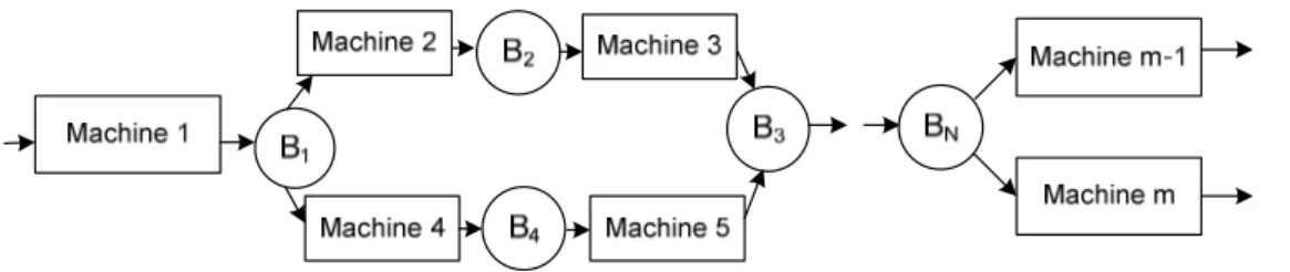
Obviously, series-parallel lines constitute a generalization of tandem lines. Figure 2 illustrates an example of a series-parallel line.
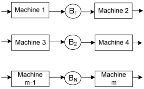
7 Many authors consider the knapsack-type problems assuming that the cost function J(H) is linear and that the minimum required production rate V 0 is given. Such problems may be considered in terms of our problem formulation assuming that the revenue function R(V(H)) is stepwise: if V(H) is above a given threshold V 0, then R(V(H)) equals to some sufficiently large constant M, otherwise R(V(H))=0. This knapsack-type problem for series-parallel lines turns out to be NP-hard. Again, to prove this, we need to have a procedure that computes the average production rate in polynomial time. It will be sufficient for us to present such a procedure only for series-parallel lines with a simple structure. By system with a simple structure, we mean any line which is represented by a digraph G consisting of paths starting at vertex v0 and ending at vertex vN+1, where
each path consists of 2 arcs and different paths do not have any other common vertices except for v0 and vN+1. An example of a system with simple structure is provided in
Figure3.
Figure 3. Example of a series-parallel line with simple structure (several two-machine tandem lines in parallel)
The input data of a problem instance consist of graph G, parameters
λ
i,µ
i, ui, i=1,…,m,dj, j = 1,…,N and Tam. The functions R(V) and J(H) are given by parameters dj,
j = 1,…,N, V 0 and M. Equivalently, one can neglect the functions R(V) and J(H) and
consider the problem of minimizing the function
∑
= N j j jh b 1
, subject to the constraints
8
Proposition 2. The problem of finding a buffer capacity allocation vector H = (h1,
h2,…, hN)∈Z+N minimizing the function
∑
= N j j jh b 1
, subject to the constraints V(H) ≥ V 0,
h1 ≤ d1, h2 ≤ d2,…, hN ≤ dN for a series-parallel line with a simple structure and rational
weights b1,…, bN, V 0 and
λ
i,µ
i, ui, i= 1,…,m, is NP-hard.Proof. See (Dolgui, Eremeev, Sigaev, 2007).
Let us now consider minimization of the average steady state inventory cost function Q(H). The input data of a problem instance with this criterion consist of graph G, parameters
λ
i,µ
i, ui, i = 1,…,m, dj, j = 1,…,N and Tam. The functions R(V) and Q(H) aregiven by parameters dj, cj, j = 1,…,N, V 0 and M. Again, one can neglect the functions
R(V) and Q(H) and consider the problem of minimizing the function
∑
= N j j jq H c 1 ) ( ,subject to the constraints V(H)≥ V 0, h1 ≤ d1, h2 ≤ d2,…, hN ≤ dN. Computational
complexity of this knapsack-type problem is considered below.
Proposition 3. The problem of finding a buffer capacity allocation vector H=(h1, h2,…,
hN)∈Z+N minimizing the function
∑
= N j j jq H c 1 )
( , subject to the constraints V(H) ≥ V 0,
h1 ≤ d1, h2 ≤ d2,…, hN ≤ dN for a line with a simple structure and rational weights
c1,…,cN, V 0 and
λ
i,µ
i, ui, i = 1,…, m, is NP-hard.Proof. Consider a special case of the problem with m=2N, where each path consists of
two sequential machines indexed i,i+1, for all odd i, 1 ≤ i ≤ N. Let j = (i+1)/2 be the index of the buffer between machines i and i+1. Assume also that
λ
i=2 ui ,µ
i=4ui for alli=1,…,m, d1= d2=…= dN=1 and ui = ui+1 for all odd i.
In a line with simple series-parallel structure considered here, all pairs of sequential machines work independently from each other, so the steady-state throughput of such a pair and the steady-state average number of parts in the buffer between the machines depend only on parameters of the two machines. Let V’j be the throughput of the
9 Forestier, 1982) in case hj=1 we obtain: V’j=8u2j/13, and if hj=0, we have: V’j=u2j/2,
j=1,…,N.
Machines within each pair have identical parameters, so qj(H) = 1/2 hj (see the
Appendix). In the case hj=1 holds qj(H)=1/2, and when hj=0, we have qj(H)=0, j=1,…,N.
The throughput of the whole system is V(H)=V’1+ V’2+…+ V’N. Therefore, all the
necessary system parameters are computable in polynomial time.
To show the NP-hardness we will again use the Partition problem, see Proposition 1.
We set N = n , u2j= u2j+1 =aj26/3, cj=2aj, j = 1,…,N and V0= ∑
= N j j a 1 6 29 . In case hj=1 we
have V’j= aj⋅16/3, qj(H)= aj and otherwise V’j= aj⋅13/3, qj(H) =0, j=1,…,N.. Therefore
the total throughput is
V(H)=
∑
= N j j V' 1 =∑
= N j j jh a 1 +∑
= N j j a 1 3 13 =∑
= N j j jh a 1 + V 0 -∑
= N j j a 1 2 1 .So, H∈{0,1}N is feasible if and only if
∑
= N j j jh a 1 ≥
∑
= N j j a 1 2 1. It is easy to see that the
Partition problem has the affirmative answer if and only if
∑
∑
= = = N j j j N j j jq H a h c 1 1 ) (
≤
∑
= N j j a 1 2 1. Therefore the special case of buffers capacity allocation problem considered in
this proposition is NP-hard. □
3. Conclusion
In this paper, we have proven NP-hardness of the buffer capacity allocation problem for two cases: 1) tandem production lines with oracle representation of the revenue and cost functions, and 2) series-parallel lines of simple structure with stepwise revenue function.
Acknowledgments
The research is partially supported by Russian Foundation for Basic Research grants 07-01-00410 and 12-01-00122, by Presidium RAS (project 15.8) and SB RAS (project 7B). The authors thank Chris Yukna for his help with English.
10 In this appendix we describe the production line model used for two-machine line analysis, i.e. when the number of buffers is N=1 and the number of machines is m=2 (Dubois and Forestier, 1982). Let h be the capacity of the buffer between the machines. In this case the system states can be expressed by the triple (α1,α2,x), where αi =0 if machine i is under repair, and αi =1 if it is operational. The value x∈ [0,h]
denotes the amount of buffer capacity used by the parts. In this discrete-continuous model for the two-machine serial system we have a set of intermediate states {0,1}2 × ] 0, h [ and the boundary states ({0,1}2×{0})∪({0,1}2×{h}). Let Ai denote the binary random variable for the state of machine i, i=1,2, and let X be the random variable for the amount of buffer capacity used by the parts. The probabilistic characteristics in this model are given by the probabilities of boundary states at time t:
Pα1α2(0,t)=P{(A1, A2,X)=(α1,α2,0) at time t},
Pα1α2(h,t)=P{(A1, A2,X)=(α1,α2,h) at time t},
and the probability density fα1α2(x,t) of intermediate states: fα1α2(x,t)=∂Fα1α2(x,t)/∂x, where Fα’1α’2(x,t)
is the probability that at moment t the system state (A1 ,A2 ,X) is such that A1=α1, A2=α2, and X < x. The
asymptotic steady-state distributions are described by
Pα1α2(0)=limt→∞Pα1α2(0,t), Pα1α2(h)=limt→∞Pα1α2(h,t),
fα1α2(x)=limt→∞fα1α2(x,t).
We use the asymptotic relationships obtained in (Dubois and Forestier, 1982). For the intermediate states we have:
0=λ1f10(x)+ λ2f01(x)-(µ1+µ2)f00(x),
-u2 ∂f01(x)/∂x=λ1f11(x)+ µ2f00(x)-(µ1+λ2)f01(x),
u1 ∂f10(x)/∂x=λ2f11(x)+µ1f00(x)-(λ1+µ2)f10(x),
(u1-u2)∂f11(x)/∂x=µ1f01(x)+µ2f10(x)-(λ1+λ2)f11(x)
For the boundary states three cases should be considered: u1>u2, u1<u2 and u1=u2=u. We use only the
latter case, where the following equations can be proved:
P01(h)=P00(h)= P10(0)=P00(0)=0,
µ2P10(h)= λ2P11(h)+ uf10(h)=(λ1+λ2)P11(h),
µ1P01(h)= λ1P11(0)+ uf01(0)=(λ1+λ2)P11(0),
u f01(h)= λ1P11(h), uf10(0)= λ2P11(0).
Solution of this system yields the analytic expressions for fα1α2(x), Pα1α2(0), and Pα1α2(h). Using these functions one can obtain the average production rate V(h). For example in case λ1=λ2=λ, µ1=µ2=µ we
have:
F10(x)=kx, F00(x)=kxλ/µ, F11(x)=kxµ/λ, F01(x)=kx,
P11(h)=ku/λ, P10(h)=2ku/µ, P00(h)= P01(h)=0,
P11(0)=ku/λ, P01(0)=2ku/µ, P00(0)= P10(0)=0, where k is found from normalization condition
∑
∈ ∈ } 1 , 0 { }, 1 , 0 { 2 1 α α [Fα1α2(h) + Pα1α2(h)+ Pα1α2(0)] = 1.
In the complexity analysis within this paper we employ only the case where µ1=µ2 and λ1=λ2. Let
I=µ1/λ1=µ2/λ2. Then the average production rate is given by:
1 2 1 2 1 ) ( ) 1 ( 1 1 ) ( − + + + + + = u I h I I u h V µ µ µ µ .
11 The value Q(H) can be found by summing the expected amounts of parts (multiplied by the inventory costs) in buffers. In particular, for a two-machine tandem line as considered above, the steady state average number of parts in the intermediate buffer q is derived as follows. For any of the four combinations of the indices α1∈{0,1}, α2∈{0,1} at any moment t we can define a random value
Z(α1,α2), assuming Z(α1, α2)= X, if the system is in a state (A1,A2,X), such that A1=α1, A2=α2 ;
otherwise Z(α’1,α’2)=0.
Asymptotically, as t tends to ∞, the distribution function for each random variable Z= Z(α1, α2),
α1∈{0,1}, α2∈{0,1}, is FZ (x)=P{Z<x}=P{Z<x & (A1, A2) =(α1 ,α2)} + P{Z<x & (A1, A2) ≠(α1 ,α2)}. Note that
{
}
{
}
= ≤ = = < otherwise A A P h x if x F A A x Z P , ) , ( ) , ( , ), ( ) , ( ) , ( & 2 1 2 1 2 1 2 1 2 1α
α
α
α
α α by definition of Fα1α2(x), and{
}
{
}
= − ≤ = ≠ < . , ) , ( ) , ( 1 , 0 , 0 ) , ( ) , ( & 2 1 2 1 2 1 2 1 otherwise A A P x if A A x Z Pα
α
α
α
Thus, in view of properties of expectation (see e.g. (Gnedenko, 1997)), using the definitions of
Fα1α2(x) and Pα1α2(h) and the fact that FZ (x)≡1 for x>h , we obtain
E[Z] =
∫
∞ 0 [1-FZ (x)] dx =∫
h 0 [1-FZ (x)] dx =∫
h 0[
1- Fα1α2(x) – 1+P{(A1, A2)=(α1,α2)}]
dx=[
F h P h F x]
dx h∫
+ − 0 ) ( ) ( ) ( 2 1 2 1 2 1α αα αα α , and in total,[
]
∑
∑ ∫
∈ ∈ ∈ ∈ ⋅ + − = } 1 , 0 { }, 1 , 0 { } 1 , 0 { }, 1 , 0 { 0 2 1 2 1 2 1 2 1 2 1 ( ) ( ) ( ). α α αα α α αα αα h P h dx x F h F q hWith u1=u2=u, µ1=µ2 and λ1=λ2 it yields q = h/2.
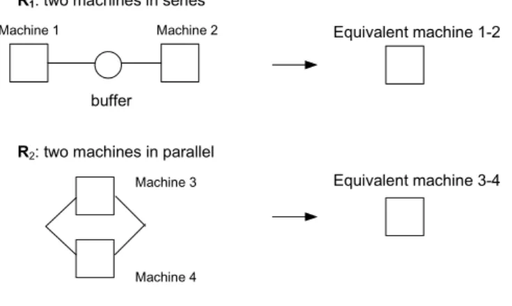
The above model is developed for two machines with a buffer in between. For a series-parallel line with more machines and buffers, the aggregation algorithm for production rate evaluation consists in applying the following two rules:
R1:two machines in series are replaced with an equivalent machine
R2 : two machines in parallel are replaced with an equivalent machine
The parameters λ*, µ*, u* of the equivalent machines are calculated from differential equations
12 parallel machines (R2). More details on these equations may be found in (Dolgui, 1993; Dolgui et al. 2002, 2007).
After K-1 steps of such aggregation procedure the system reduces to a single machine with parameters λ*
, µ*, u* and the estimate of the overall production rate V(H) is given by u*µ*/(λ*+µ*).
The precision of this approximate method depends on the order in which the line is aggregated. In our study, the replacement of type R1 is always applied where possible before the reduction of type R2.
Machine 1 Machine 2
buffer
R1: two machines in series
R2: two machines in parallel
Machine 3
Machine 4
Equivalent machine 1-2
Equivalent machine 3-4
Fig. A1 Decomposition rules
In case there are several alternatives, the rule R1 is applied to the couple of machines, separated by a
buffer of the least capacity. The value Q(H) is estimated by summing the expected amounts of parts (multiplied by the inventory costs) in buffers being eliminated on each step of aggregation.
References
Cheng T.C.E., Kovalyov M. Y. (2002) An unconstrained optimization problem is NP-hard given an oracle representation of its objective function: a technical note, Computers & Operations Research 29, 2087–2091.
Coillard P. and Proth J.M. (1984) Effet des stocks tampons dans une fabrication en ligne, Revue belge de Statistique, d’Informatique et de Recherche Opérationnelle
24 (2), 3-27.
Dallery Y. and Gershwin S.B., (1992) Manufacturing flow line systems: a review of models and analytical results, Queueing Systems 12 (1-2), 3-94.
Dolgui A. (1993) Analyse de performances d'un atelier de production discontinue: méthode et logiciel, Research Report INRIA 1949, 44 pages.
Dolgui A., Eremeev A.V., Kolokolov A.A., Sigaev V.S. (2002) A genetic algorithm for allocation of buffer storage capacities in production line with unreliable machines. Journal of Mathematical Modelling and Algorithms 2, 89-104.
13 Dolgui A., Eremeev A.V., Sigaev V.S. (2007) HBBA: hybrid algorithm for buffer allocation in tandem production lines. Journal of Intelligent Manufacturing 18 (3), 411-420.
Dolgui A.B. and Svirin Y.P. (1995) Models of evaluation of probabilistic productivity of automated technological complexes, Vesti Akademii Navuk Belarusi: phisika-technichnie navuki, n°1, 59-67 (in Russian).
Dubois D. and Forestier J.P. (1982) Productivité et en-cours moyens d’un ensemble de deux machines séparées par une zone de stockage, RAIRO Automatique 16 (2), 105-132.
Garey M.R. and Johnson D.S. (1979) Computers and Intractability. A Guide to the theory of NP-completeness, W.H. Freeman and Company, San Francisco.
Gershwin S.B. (1993). Manufacturing Systems Engineering, Prentice Hall.
Gershwin S.B. and Schor J.E. (2000) Efficient algorithms for buffer space allocation, Annals of Operations Research 93, 117-144.
Gnedenko B.V. (1997) Theory of probability, Gordon and Breach, Amsterdam.
Heavey C., Papadopoulos H.T. and Browne J. (1993) The throughput rate of multistation unreliable production lines, European Journal of Operational Research 68, 69-89.
Levin A.A. and Pasjko N.I. (1969) Calculating the output of transfer lines, Stanki i Instrument 8, 8-10 (in Russian).
Li J. and Meerkov S.M. (2008) Production Systems Engineering, Springer.
Sevast'yanov B. A. (1962) Influence of storage bin capacity on the average standstill time of a production line, Theory Probab. Appl, 7 (4), 429–455
So K.C. (1997) Optimal buffer allocation strategy for minimizing work-in-process inventory in unpaced production lines, lIE Transactions 29, 81-88
Shi C. and Gershwin S. B. (2009) An efficient buffer design algorithm for production line profit maximization Original Research, International Journal of Production Economics 122 (2), 725-740
Smith J.M. and Daskalaki S. (1988) Buffer space-allocation in automated assembly lines. Operations Research 36, 343-358.
14 Tan B. and Gershwin S.B. (2009) Analysis of a general Markovian two-stage continuous-flow production system with a finite buffer, International Journal of Production Economics 120 (2), 327-339.
Terracol C. and David R. (1987). An aggregation method for performance valuation of transfer lines with unreliable machines and finite buffers, Proceedings of the IEEE International Conference on Robotics and Automation, 1333–1338.