Cingulate-Hippocampus Coherence and Trajectory Coding in a Sequential Choice Task

(1)

Cingulate-Hippocampus Coherence and

Trajectory Coding in a Sequential Choice Task

The MIT Faculty has made this article openly available.

Please share

how this access benefits you. Your story matters.

Citation

Remondes, Miguel, and Matthew A. Wilson.

“Cingulate-Hippocampus Coherence and Trajectory Coding in a Sequential

Choice Task.” Neuron 80, no. 5 (December 2013): 1277–1289.

As Published

http://dx.doi.org/10.1016/j.neuron.2013.08.037

Publisher

Elsevier

Version

Author's final manuscript

Citable link

http://hdl.handle.net/1721.1/102690

Terms of Use

Creative Commons Attribution-NonCommercial-NoDerivs License

(2)

Cingulate-hippocampus Coherence and Trajectory Coding in a

Sequential Choice Task

Miguel Remondes and Matthew A Wilson

The Picower Institute for Learning and Memory, Department of Brain and Cognitive Sciences, Massachusetts Institute of Technology, Cambridge, MA, USA

Abstract

Interactions between cortex and hippocampus are believed to play a role in the acquisition and maintenance of memories. Distinct types of coordinated oscillatory activity, namely at theta frequency, are hypothesized to regulate information processing in these structures. We

investigated how information processing in cingulate cortex and hippocampus relates to cingulate-hippocampus coordination in a behavioral task where rats choose from four possible trajectories according to a sequence. We found that the accuracy with which cingulate and hippocampal populations encode individual trajectories changes with the pattern of cingulate-hippocampal theta coherence, over the course of a trial. Initial theta coherence at ∼8Hz during trial onsets lowers by ∼1Hz as animals enter decision stages. At these stages, hippocampus precedes cingulate in processing increased amounts of task-relevant information. We hypothesize that lower theta frequency coordinates the integration of hippocampal contextual information by cingulate neuronal populations, to inform choices in a task-phase dependent manner.

Introduction

All organisms need to constantly gather and update information about their inner states and surrounding contexts, in order to make informed decisions regarding their daily actions. This process involves the encoding and storage of information by neurons, as memory. The hippocampus (HIPP) has been implicated in the encoding and retrieval of memories (Scoville & Milner 1957) whose content often joins complex multi-modal sensory

representations, such as spatial locations (O’Keefe & Dostrovsky 1971; Ekstrom et al. 2003; Kreiman et al. 2000), feelings (LeDoux 1993), and abstract concepts (Kreiman et al. 2000), suggesting that hippocampus-dependent memories integrate information from distinct extra-hippocampal sources. Coordinated activity between extra-hippocampal formation (HIPP), mammillary bodies, thalamus, and cortex, forming the Papez circuit, is believed to support mnemonic functions by regulating the transfer of information between distant brain structures (Battaglia et al. 2011; Belluscio et al. 2012; Buzsaki 1989; Jones & Wilson 2005; Siapas et al. 2005; Remondes & Schuman 2002). Within this circuit, cingulate cortex (CG) is modeled as an executive memory hub, maintaining a map of relations between actions, outcomes an contexts (Teixeira et al. 2006; Vetere et al. 2011; Wang et al. 2012; Durkin et al. 2000; Foster et al. 1980), with the capacity of signaling errors and suppressing

Correspondence: remondes@mit.edu.

Publisher's Disclaimer: This is a PDF file of an unedited manuscript that has been accepted for publication. As a service to our

NIH Public Access

Author Manuscript

Neuron. Author manuscript; available in PMC 2014 December 04.

Published in final edited form as:

Neuron. 2013 December 4; 80(5): . doi:10.1016/j.neuron.2013.08.037.

NIH-PA Author Manuscript

(3)

inappropriate responses (Endepols et al. 2010; Kennerley & Wallis 2009; Sul et al. 2010; Totah et al. 2009; Cowen et al. 2012; Carter et al. 1998).

We hypothesize that fine coordination with HIPP would provide CG with a permanent source of spatial contextual information (O’Keefe & Burgess 1996; Gupta et al. 2012), allowing it to update its relational map and fulfill its functions. Fine cingulate-hippocampal coordination is predictable by their anatomical connectivity (Jones et al. 2005; Jones & Witter 2007), and illustrated by the fact that both structures exhibit dynamic synchronization as animals transition between distinct behavioral states (Young & McNaughton 2009). However, it is still unknown whether CG-HIPP coordination varies with task demands or exhibits any relation with the processing of behavioral-relevant information.

We tested this hypothesis by investigating, in parallel, dynamic patterns of cingulate-hippocampal coordination, and the amount of behavioral information carried by neuronal populations’ spikes, while we challenge cingulate executive functions under complex contingencies. We developed a novel task, the Wagon-wheel Maze (WWM), in which rats choose sequentially from four trajectories for a reward. We then decoded activity from CG and HIPP and found that both populations carry increased trajectory information as animals move towards choice points. We then asked whether these changes in information content are reflected in distinct patterns of CG-HIPP coordination. We found that, as animals progress to choice points, CG-HIPP coherence of the local field potential (LFP) is initially dominated by theta at a high-frequency (8–10 Hz, HIGH-theta), and lowers by ∼ 1Hz as animals run the maze’s outer circle where cues defining each choice become available. This change is accompanied by increases in the amount of trajectory information encoded by CG and HIPP neurons, with HIPP increasing earlier than CG, coincident with periods of wide-band theta coherence (5–10 Hz, WIDE-theta). Lastly, we investigated the relative timing and G-causality between HIPP and CG spikes and LFP, and found distinct patterns of CG-HIPP coordination across WWM stages, as well as a bias for HIPP to G-cause CG neural activity. We hypothesize that lower theta frequencies at choice stages regulate increased information flow from HIPP to CG, to enhance trajectory coding and inform behavioral choices.

Results

Rats learn and memorize sequences of trajectories on the WWM

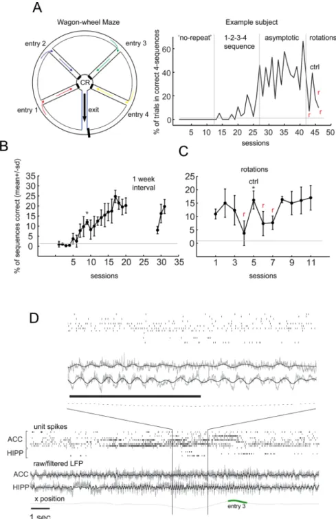
The WWM is a win-shift task that joins aspects of traditional T-maze and of radial maze tasks. As depicted in Figure 1A each trial starts as the rat exits the CR area (“center reward” area - the wheel hub), progresses through EA, and turns left towards the outer circle (OC) facing the different choices (“entries” 1 through 4 in Figure 1A), each marked by local, as well as distal room cues, defining each trajectory. Faced with 4 different choices, the rat must choose the correct one according to a sequence rule (entries 1–2–3–4), in order to receive a liquid chocolate reward. It follows from this arrangement that a correct sequence is composed of 4 trajectories with extensive commonalities (segments EA, CS2 and CS3, Figure S2C).

Training rats in a simple win-shift version of the task for ∼2 weeks does not generate sequential behavior, in spite of a high (60–100) number of trials per 20–30 min daily session (“no-repeat” on Figure 1A). Once we introduce the sequence-rule, subjects gain significant proficiency over a period of 15–21 days, eventually reaching asymptotic levels (Figure 1A– B). Over this period, single unit, LFP and position data were recorded throughout the task (Figure 1D), using a multi-tetrode drive (Figure S1).

A one-week break in training causes a drop in proficiency, not present on a subsequent testing session, indicating that subjects kept memory of the task (Figure 1B). In order to test

NIH-PA Author Manuscript

(4)

WWM dependency on allocentric cues, we trained a different group of subjects to

asymptotic levels, and performed probe sessions with the maze rotated by 180° (red-colored “r” on Figure 1A and C). Lower proficiency under this manipulation contrasts with the lack of effect obtained when we swap the local cues placed at each choice point (data not shown), indicating that WWM performance relies on distal cues.

HIPP and CG neural populations increase trajectory information across consecutive WWM stages

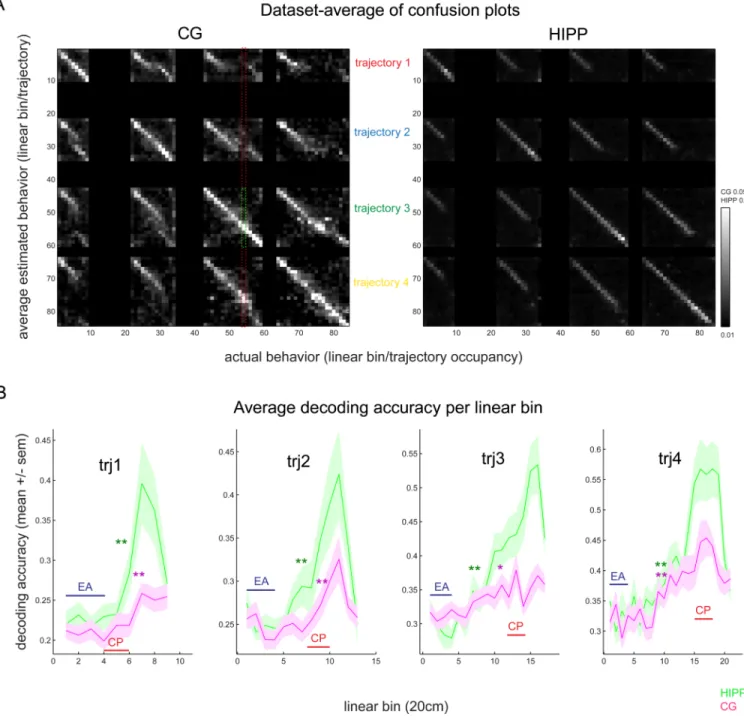
CG neurons have been shown to report aspects of error and reward signaling and effort-based decision making (Bryden et al. 2011; Endepols et al. 2010; Liu et al. 2009; Sul et al. 2010; Totah et al. 2009; Cowen et al. 2012). In order to study the dynamics of CG and HIPP population coding of WWM choices, we used a Bayesian decoding framework in which we estimate the animals’ position and trajectory at each consecutive time bin, given the multiple single-unit population firing rate distribution. As explained in Methods, we used each session’s spike and position data (Figure 2A–B top and mid-panel) to compute single-neuron behavioral tuning curves (rate maps) for each linear bin on each trajectory, and estimated the animal’s behavior given the behavioral tuning curves, at consecutive 250ms bins of a session. Examples of these Bayesian estimates are depicted on Figure 2 for CG (A) and HIPP (B) neuronal populations. At each consecutive 250ms bin (on the XX axis), the probability of the rat being either in bins 1:9 of trj1 (1.8 m long), bins 1:13 from trj2 (2.6 m), bins 1:17 from trj3 (3.4 m) or bins 1:21 from trj4 (4.2m), is linearly arranged down the YY axis. In order to visually compare the estimated with the real behavior, Figure 2 estimates were overlaid with a “behavior map” (in red) containing the real recorded occupancy (linear bin/trajectory) on each consecutive 250ms bin.

In order to validate the decoding process and quantify the decoding accuracy from each of the two regions, we built the decoder’s ratemap using half the session’s trials, and decoded the other half of the session’s trials (see Methods). We subsequently compared the

Bayesian-estimated with the actual behavior of the rat, by building a confusion plot (Figure 3A). This plot depicts the average decoded behavior corresponding to each of all possible behavior occupancy states. Estimation errors correspond to increased density off the diagonal areas. For each dataset’s confusion plot, the probability corresponding to correctly estimated behavior (diagonal), divided by the marginal total probability corresponding to each consecutive behavioral state (on the YY axis), represents how accurately each neural population identifies trajectory on each consecutive linear bin (decoding accuracy - Figure 3B). Analogous reasoning was applied in the time-bin decoding from subsequent analyzes. We computed this value for each dataset, and summarized values across all datasets on both brain regions, plotting the data against position (linear bin), in Figure 3B. On both areas there is a significant increase in estimation accuracy as animals exit the start region (EA) and travel on the maze perimeter (beyond EA), where allocentric spatial cues define distinct entry points. HIPP accuracy in estimating the trial’s trajectory increases earlier, and reaches significantly higher levels, than CG’s (Figures 3, 5A and Figure S3). This suggests that choice-relevant spatial information is first concentrated in HIPP, and then conveyed to CG, leading us to investigate the nature of CG-HIPP coordination over trial stages.

The frequency of CG-HIPP LFP theta coherence changes during WWM trials

Coordinated oscillations are widely considered crucial for behavior, insofar as they govern communication between remotely located neuronal networks processing distinct

information. The frequency of HIPP theta changes under increased cognitive demands and sensorial information load, as well as novel contexts (Sainsbury et al. 1987; Bland et al. 1995; Kay 2005; Jeewajee et al. 2008). In order to investigate CG-HIPP oscillatory activity

NIH-PA Author Manuscript

(5)

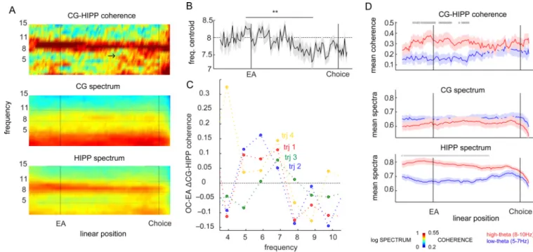
at distinct behavioral phases, and study their relationship with the dynamics of trajectory coding, we computed the coherence between CG and HIPP LFP, over the course of trials. We saw significant changes in the patterns of CG-HIPP coherence patterns as rats progress on the WWM (Figure 4A–B, for Trajectory 3, see Figures S3–S4 for all four trajectories). Coherence within the theta band shows a temporal distribution, in which the start arm (up to EA in the plots) is characterized by theta frequencies that span from 8 to 11Hz, with a centroid around 8.2Hz (Figure 4A top panel, and B). Later, as animals travel the perimeter towards CP (labeled “Choice” in the axis), theta coherence changes to include low theta frequencies, and lowering the mean frequency by ∼1.0 Hz (Figures 4B, and S3 fourth row). These variations led us to investigate which coherence frequencies change while the animal transitions from trial onset to the maze perimeter, and how. We thus plotted the normalized coherence difference (delta-coherence = (POC − PEA)./(POC + PEA)) between the last 30cm

of the start arm (EA, 0.6 to 0.9 m of linearized position), and the first 30cm of the outer circle (OC, 0.9 to 1.2m of linearized position) against individual frequency bins (Figure 4C). We found that coherence decreases at frequencies above and including 8Hz, and increases below this number, strictly within the theta range. We thus used 8Hz as our high-low theta cutoff for subsequent analyses. In order to study in detail the dynamics of high and low theta coherence, over the course of trials, we averaged coherence within each of the theta bands, and compared the two coherencies over consecutive linear positions (Figure 4D, TRJ3, please see Figure S3 for all other trajectories). We found a significant difference between low (5–7Hz) and high (8–10Hz) theta coherence at trial onsets (EA), followed by equal coherencies at the outer circle, and a decrease in the mean coherence frequency (Figure 4D, TRJ3, please see Figure S3 for all other trajectories). CG theta is less well documented than HIPP theta, and seems to be less intense (Figure 4A, TRJ3, please see Figure S3 for all other trajectories) (Young & McNaughton 2009). In a manner analogous to the previous

coherence analysis, in Figure 4A (and S3) we plotted the dataset-averaged normalized spectral density of both HIPP and CG LFP, and on Figure 4D (and S4) we did it separately for HIGH and LOW theta frequency bands. This analysis shows an interesting feature of CG theta. While HIPP theta is dominated mostly by high frequency (8–10Hz), up to choice points were HIGH and LOW frequencies become equally powerful, CG exhibits equal power at both frequency ranges throughout the task (Figures 4D, S3).

Thus, while animals run a WWM trial, CG-HIPP theta coherence exhibits two distinct regimes. At trial initiations theta coherence is dominated by high frequencies (8–10Hz), with a centroid at 8.2+/−0.2 Hz. Upon entering the outer circle, where environmental cues characterize each choice and information processing levels increase both at CG and HIPP (Figure 3), theta coherence changes to a wide-frequency mode (WIDE-THETA), with a net decrease in the mean frequency of theta coherence (Figure 4B–D, S3 third and fourth rows). We should point out that equivalent analyses made for lower frequencies (1–4 Hz), also shown to be present in HIPP, mPFC and VTA (Fujisawa & Buzsaki 2009), do not show comparable differences in coherence nor spectra (Figure S6), in agreement with the previous analysis (Figure 4C, and comments above).

Consecutive WWM behavioral stages are characterized by distinct theta coherence, matching distinct trajectory information processing

Since both neural coding and neural coordination globally change as subjects move towards the WWM perimeter, we hypothesized that distinct theta coherence regimes would serve distinct cognitive functions in the WWM task. Namely, under increased behavior-relevant contextual information, coherence would shift towards lower theta frequencies (Sainsbury et al. 1987; Bland et al. 1995; Kay 2005; Jeewajee et al. 2008), typical of CG (Figure 4A–D, mid panels). This change would open a communication channel between CG and HIPP, through which relevant contextual information would flow from HIPP to CG. If this

NIH-PA Author Manuscript

(6)

hypothesis is correct, two predictions can be made: a) CG and HIPP trajectory information should increase in the WWM regions characterized by WIDE-THETA and, b) HIPP activity should precede CG’s. To test the first prediction, we decoded CG and HIPP single-unit data corresponding to the same time intervals used in the previous coherence analysis. For this we computed decoding accuracy on 50ms-shifted 1sec time windows, for each individual trajectory (see Methods). Figure 5A (lower panel) depicts the mean trajectory information computed as before, but now with behavioral tuning curves computed in time instead of linear position, and behavior estimated on 50-ms sliding, 1 sec windows (see Methods). Consistent with the previous analyses (Figure 3), trajectory information increases from EA to outer circle stages, earlier in HIPP relative to CG (Figure 5A lower panel). This dynamic resembles that from LFP theta coherence (Figure 5A, top panel), such that WIDE-THETA periods, characterized by coherence at lower theta-frequency, correspond to increased trajectory information (Figure 5A, trajectory3, please see Figure S3 for all trajectories). In order to compare CG-HIPP coherence and trajectory information levels at distinct WWM stages, we took the average CG and HIPP LFP coherence, spectra, and trajectory

information content, in the last 0.5 sec of EA (trial onset, labeled EA in the plots) and in the last 0.5sec of OC segments for each trajectory (decision stage, labeled “Choice”, and OC in the bar plots). In line with our initial observations, distinct WWM stages correspond to significantly different levels of information processed (Figure 5B, top), and lower average theta coherence frequency (Figure 5B, bottom). This is in agreement with different levels of coherence at HIGH and LOW-theta, on EA but not OC (Figure 5C, left). CG and HIPP LFP theta spectra, measured at equivalent WWM stages, confirms the marked differences we’ve seen before, with HIPP theta dominated by high frequencies, regardless of WWM stage (Figure 5D, bottom panel). To further test a connection between CG-HIPP coherence regimes and the levels of information processed by CG and HIPP, we compared the absolute values, as well as increments, of each dataset’s average trajectory information during periods of WIDE-THETA versus periods of HIGH-THETA. We found that the average trajectory information content increases, in both CG and HIPP, as animals change from maze locations characterized by HIGH-THETA to those characterized by WIDE-THETA (Figure S5C, top panel), with increments of 16 and 19%, respectively for CG and HIPP (Figure S5C, bottom panel). Equivalent increments were found when we compared trajectory information at WIDE-THETA with the one at HIGH-THETA, defined on the basis of mean frequency centroid. Periods of decreased theta-coherence frequency

correspond to increased CG and HIPP trajectory information (Figure S5B). Lastly, we tested the connection between CG-HIPP coherence at the two theta frequency bands, and levels of decoding accuracy on a trial-by-trial basis. For this we computed the correlation between the single-trial accuracy and coherence values within EA and OC regions of the WWM. This analysis revealed a significant positive correlation between CG coding accuracy and coherence, restricted to LOW-THETA frequencies, and to the maze perimeter (Spearman Rho=0.11, p<0.001, Figure S8C).

We have, therefore, an overall increase in trajectory information in both CG cortex and HIPP, on WIDE vs HIGH theta coherence regimes, corresponding to stages of the WWM marked by distinct cognitive demands. In addition, we have a significant, positive correlation between the amount of CG information processed at the WWM perimeter, and LOW-THETA coherence. These analyses confirm our first prediction: HIPP and CG trajectory information increases from trial onset to decision stages, with a corresponding drop in the frequency of theta coherence, whose value at LOW-theta determines the level of trajectory information processed by CG. We have still to test the second prediction, namely whether HIPP neural activity precedes CG’s, and whether we can measure any form of causal flow between the two structures, as our analysis of decoding dynamics suggests

NIH-PA Author Manuscript

(7)

(Figures 3B and 5A: precedence of HIPP over CG in processing increased trajectory information).

HIPP functionally precedes CG over distinct regions of the WWM

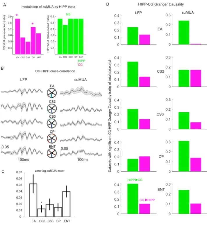
In order to investigate temporal patterns of functional connectivity between CG and HIPP, we started by asking whether CG and HIPP multi-unit activity (suMUA) are modulated by HIPP theta. For this we extracted the phase of band-pass (theta) filtered HIPP LFP, and then the HIPP theta phase of each suMUA spike (see Methods). Then, for each region of the maze, we asked whether suMUA was biased by the HIPP theta rhythm, using a Rayleigh’s test for non-uniformity of phases’ distribution. Figure 6A depicts a color-coded bar plot showing, for each WWM region, the percentage of datasets in which suMUA was

significantly biased by the HIPP theta rhythm. In the majority of datasets both HIPP and CG spikes are indeed significantly biased by HIPP theta (HIPP 80–90% and CG 60–80%). Across datasets we found a mean preferred phase of 102.6+/−63° for CG and 153+/−36° for HIPP (not different) spikes, indicating that CG and HIPP spikes occur, on average, in the descending phase of HIPP LFP theta. Importantly, the % of significantly modulated CG, but not HIPP, datasets, exhibits significant variations with WWM regions. The first of these periods is the EA, in which 86% of all datasets show significant modulation of CG spikes by HIPP theta, followed by a significant drop at outer circle segments (CS2 and CS3), in which 57 and 50% of datasets show significant modulation, and a final recovery at choice segments (CP), to levels equivalent to EA. We do not see such variation in HIPP spikes, as most datasets exhibit modulation by theta throughout the maze. The fact that both CG and HIPP neurons fire during the descending phase of the HIPP theta wave, and that, depending on the WWM region considered, CG spikes are variably likely to be significantly modulated by theta, suggests the existence of distinct modes of CG and HIPP joint coordination by HIPP theta, in agreement with our coherence results.

In order to examine the relative timing of CG and HIPP activity, we computed, for each of the distinct WWM partitions, the MUA and LFP cross-correlation profile between CG cortex and HIPP (Figure 6B, see Methods). Most of the cross-correlograms have clear peaks that occur at a theta frequency, something also seen in suMUA-LFP correlograms on all WWM regions (Figure S7C), supporting prominent CG-HIPP theta coordination, and suggesting that HIPP spikes precede CG depolarization and local dendritic computations. Importantly, at trial onsets (EA), HIPP and CG spikes tend to be largely simultaneous, the two region’s spikes aggregating at zero time-lag of each other (Figure 6B–C). As animals move towards the outer circle, a HIPP-CG lag of about 80ms develops, changing the average zero-lag cross-correlation from 0.052+/−0.012 at EA, to 0.01+/−0.005 at CS2 (Figure 6C).

The previous analysis demonstrates theta-regulated coordination between CG and HIPP activity, with HIPP preceding CG. In order to test our initial hypothesis we are still to test the presence of causality between HIPP and CG neural activity. According to Clive Granger’s personal account, if knowing the values of a given variable X1 helps predict the

future values of another X2, then X1 is said to cause X2 (Clive W. J. Granger Norman R.

Swanson and Mark W. Watson 2001). How well can we predict CG from HIPP neural activity? In order to answer this question, we computed Granger causality between HIPP and CG, and respective statistical significances, using the implementation of (Seth 2010). We found that HIPP activity tends to G-cause CG’s throughout the WWM regions (Figure 6D). Datasets in which HIPP neural activity G-causes CG’s significantly outnumber the ones in the opposite sense, both for LFP and for suMUA. This further supports our initial hypothesis, by showing a default causal flow from HIPP to CG, which might underlie the

NIH-PA Author Manuscript

(8)

transfer of contextual information is this direction, in agreement with the precedence of increased HIPP trajectory information over CG’s (see above and Figures 3-S3).

Discussion

Oscillations at theta frequency are hypothesized to be involved in the storage of complex representations of space and time (Belluscio et al., 2012; Buzsaki and Draguhn, 2004), as they have been shown to regulate the behaviorally-structured firing of place-selective neurons in rodents during wakefulness (Skaggs et al. 1996; Harris et al. 2003), and REM-sleep (Louie & Wilson 2001). Theta rhythms are modeled as the functional substrate on which items are encoded and retrieved together as a neural construct, with distinct frequencies postulated to carry distinct types of information (Lisman & Buzsaki 2008; Belluscio et al. 2012; Buzsaki & Draguhn 2004; Jeewajee et al. 2008).

CG cortex is strategically located at an interface between the HIPP formation and

supplementary motor areas (Jones et al. 2005; Jones & Witter 2007). It is known to encode value-cost associations (Endepols et al. 2010; Kennerley & Wallis 2009; Sul et al. 2010; Totah et al. 2009; Cowen et al. 2012), and to store contextual memories (Frankland et al. 2004; Maviel et al. 2004). We hypothesize that CG cortex fulfills fundamental roles in integrating spatial contextual information, in order to encode distinct choices, and possibly routing this information to other brain areas where a behavioral response is produced. We analyzed neural activity simultaneously in HIPP and CG cortex, in a task where rats choose freely from distinct trajectories, and are rewarded for performing them in a particular sequence, choosing the correct one, but also avoiding errors. We reasoned this task would tax CG control of behavior, known to be present in situations of cognitive conflict (Botvinick et al. 2004). Even though choice points are marked by local cues on the track, and by configurations of distal cues in the room, only the later seem critical for performance (Figure 1A, C), indicating that the rat references trajectories to spatial context. We found that CG cortical neurons signal the trajectory being performed, without exhibiting place selectivity in an open arena, in contrast with HIPP units. This indicates that CG trajectory selectivity is task-related, and not explained by hypothetical CG place selectivity.

The fact that entries are referenced to distal cues at the WWM perimeter implies that spatial information relevant to CG encoding of trajectories is processed preferentially at this stage, possibly by HIPP. We therefore predicted that CG-HIPP coordination patterns would change, as contextual information relevant to encode the distinct trajectories increases, and that a relationship between CG trajectory information and CG-HIPP coordination would develop over the course of a trial, all of which we have confirmed (Figure 5 and Figure S8). The presence of a significant change in the pattern of CG-HIPP theta coordination, linked with increased trajectory information processing, led us to hypothesize that these changes might be temporal windows of contextual information transfer between HIPP and CG. Accordingly we found that, as the frequency of theta coherence lowers, there is a significant increment in the amount of trajectory information processed, in both HIPP and CG

populations. This is consistent with studies showing decreased HIPP theta frequency in response to enhanced, novel sensory input (Sainsbury et al. 1987; Jeewajee et al. 2008), or underlying sensory-motor integration under increased cognitive demands (Bland & Oddie 1998; Kay 2005; Williams & Givens 2003). Our data suggest that spatial information encoded by HIPP at the maze perimeter is channeled to CG by lower theta frequencies. In support of this, we found that increases in trajectory information happen first in HIPP, then in CG, and that there is a positive correlation between CG accuracy and LOW-theta coherence, restricted to the maze perimeter.

NIH-PA Author Manuscript

(9)

Why would distinct levels of CG trajectory information be associated with two modes of CG-HIPP coherence? HIGH-theta rhythms dominate behaviors such as random foraging, in which active locomotion accompanies exploration, not necessarily cued to defined spatial objects (Kirk & Mackay 2003; Young & McNaughton 2009). We hypothesize that WWM trial onsets (EA) are similarly not cued to context. In fact, spatial cues necessary for mapping the upcoming trajectory are not yet present at this stage and, as a result, both brain structures process relatively little trajectory information (Figure 3B). Thus, this initial HIGH-THETA coherence mode serves the type of reward-seeking contextual exploration present during random foraging. As rats transition to the WWM perimeter, they come into contact with spatial cues relevant for choosing trajectories. At this point, contextual input from HIPP would be carried to CG by a distinct coherence mode, characterized by lower mean frequency (Sainsbury et al. 1987; Jeewajee et al. 2008). CG would now use this contextual information to encode trajectories, and might also route this information to other executive areas, namely medial prefrontal cortex, with which it is known to be coherent at lower frequencies (Young & McNaughton 2009).

Coherence, however, does not clarify the direction of trajectory information flow between HIPP and CG cortex. The results of phase modulation analysis show that CG spikes are increasingly modulated by HIPP theta at two distinct periods corresponding to distinct theta coherence modes: trial onset HIGH-theta (EA), and choice points WIDE-theta (CP). The relative timing of CG and HIPP LFP and suMUA activity shows that CG and HIPP spikes that were essentially simultaneous at EA are later offset by ∼80ms. Simultaneously, an initial EA delay of ∼70ms between HIPP spikes and CG LFP (spike-LFP

cross-correlograms, Figure S7C) becomes much shorter subsequently (∼20ms), taking up only a fraction of the HIPP-CG 80ms spikes delay. A similar difference was shown before between entorhinal inputs and HIPP targets, possibly representing local dendritic computations (Mizuseki et al. 2009), which might be present in CG as well. If this is true, HIPP spikes (rich in spatial information) would indeed provide fast depolarization of CG targets, which would locally process this information in order to encode trajectories. Finally, we

investigated the direction of a possible flow of information between HIPP and CG cortex, using Granger Causality, and found significant causal flow from HIPP to CG twice more frequently than in the opposite sense. In the context of the previous analyses, this indicates the presence of a uniform HIPP-CG causality stream, supporting the transfer of contextual information to CG.

In summary, our results show that, in a cognitively-demanding task, cingulate-hippocampus coordination determines the amount of task-relevant information processed by both regions. At trial onset rat’s behavior is not yet cued by spatial context, CG neurons process low trajectory information and the frequency of theta coherence is high. At decision stages spatial cues characterize individual trajectories; HIPP processes increased amounts of information which is conveyed to CG by a lower-frequency theta oscillation. Theta coherence mode would thus regulate a directional stream of contextual information, from hippocampus to cingulate cortex, instructing appropriate trajectory choices.

Experimental Procedures

Behavior

All procedures were performed within MIT Committee on Animal Care and NIH guidelines. Nine male Long-Evans rats (3–6 months) were used, from which 30 datasets were selected in which subjects: performed the task at above-chance levels, had stable isolated units recorded from CG cortex, and did not have tetrodes adjusted within the previous 12 hours. Subjects ran repeatedly on a wagon-wheel shaped maze from the center reward hub (CR), through the exit arm (EA), onto to the wheel perimeter (outer circle – OC, composed of

NIH-PA Author Manuscript

(10)

segments CS2–3, and CP segments), and back to the center through one of the 4 arms (ENT), in unidirectional trajectories corresponding to equal number of entries (Figures 1 and S2C). Animals were rewarded for correctly selecting one the four available reward arms, according to a set sequence (1–2–3–4). The goal of the task was to maximize the number of temporally contiguous correct choices, quantified as the % of all session’s entries pertaining to sequences of 4 correct trajectories. If an animal performs a percentage of correct

sequences significantly higher than pre-training levels, we consider it to have learned. When proficiency no longer increases, we consider it asymptotic (40–60% trials correct). Reward was administered through a long tube by an experimenter located away from the maze, behind a heavy black curtain. The maze was cleaned after each session.

Electrophysiological recordings

Data analyzed included CG and HIPP single units’ action potentials (“spikes”), local field potential recordings (LFP), and xyt position (Figure 1 D), obtained using an implanted microdrive array (Figure S1, top-left panel) of 18 independently movable tetrodes (Figure S1, top-right panel) targeting exclusively anterior CG cortex (CG, 11–9 tetrodes, 0.3 – 0.8 ML, 2.0–0.5 AP, 0–3.0 DV, mm from Bregma) and HIPP CA1 (7–9 tetrodes, 0.5 −2.5 ML, −2.0 - −4.0 AP, 3.0 DV), was surgically implanted in the rat’s skull using aseptic

techniques. Over 2–3 weeks of training we performed daily adjustment of the tetrodes. Differential recordings of extracellular action potentials (sampled at 31.25 kHz per channel, filtered between 600 Hz and 6 kHz) and continuous LFP (sampled at 2 kHz per channel, filtered between 0.1 and 475 Hz) were made against a local reference electrode in overlying white matter (HIPP), or a CG region with low amplitude LFP (CG cortex), using patch-boxes (Cheetah system) and amplifiers by Neuralynx (Tucson, AZ) as previously done in our lab (Jones & Wilson 2005). Position was acquired at 30Hz by an array of diodes located above the electrode drive. The present work included data from 9 rats, for a total of 227 CG units and 292 HIPP units, distributed over 30 datasets. Selection criteria were defined prior to any analysis other than clustering: stable recordings with single unit activity in both HIPP and CG cortex, at least 12 hours adjustment-recording lapse. At the end of the experimental period subjects were euthanized, current was passed on each tetrode, subjects were perfused intracardially, and brains were processed for histological verification of electrode location (Figure S1, bottom). CG tetrode locations were ascertained after histological analyses and, during surgery, direct visual control of the tetrode cortical entry sites, and a maximum full adjustment depth of 3 mm, until silence typical of corpus callosum was evident. Action potentials were assigned to individual neurons by offline, manual clustering based on each tetrodes’ spike amplitudes, using Xclust software (M.A. Wilson). Subsequent analyses employed a combination of in-house software (M.A. Wilson), functions from the Chronux (Bokil et al. 2010), CircStat (Berens, 2009) and GCCA (Seth 2010) toolboxes, and code written by M. Remondes, F. Kloosterman, S. Layton and D. Nguyen in C++ and Matlab (Mathworks, Natick, MA), all ultimately adapted by M. Remondes.

Bayesian decoding and CG trajectory information—We linearized individual trajectories by fitting a spline to each trajectory’s xy points, and estimating a linearized position for each xy pair. Duplets (linear_position,t) were subsequently used to extrapolate the linear positions corresponding to spike timestamps. We then divided each of the four WWM trajectories in 20 cm linear bins, to which individual spikes and individual positions were assigned for further analysis. The WWM was further divided into regions

corresponding to distinct behavioral phases, namely: the main starting segment (“EA” on Figure 1), common to all 4 trajectories, which included four linear bins from 0 to 0.8 meters of linearized trajectory, followed by the outer circle segments common to trajectories 2–4 (common segment 2 or CS2) and 3–4 (commons segment 3 or CS3) (please refer to Figure S2C). In addition, for each trajectory we defined two further segments relative to the 4

NIH-PA Author Manuscript

(11)

choice points (outer circle position in front of each entrance): CP (“choice point”, located in the outer circle) from 0.6 m before, to the actual choice point, and ENT (“entry arms”) from each choice point to 0.4 m into its facing arm (Figure S2C). The previous sectioning was used for what is referred to in the text as “linear-bin” and “region” analysis (Figure 3). In order to measure the amount of behavioral information encoded by CG neuronal populations throughout each WWM session, we estimated the conditional probability of the animal being at any given linear bin of any given trajectory, given the spiking activity from populations of multiple single-neurons (Bayesian decoding). Single-neuron behavioral tuning curves for each trajectory were computed using the above linearized position data, as follows: the number of single neuron spikes contained in each of consecutive 20cm bins was divided by the total number of position timestamps within the same linear bin, to compute that unit’s occupancy-corrected linear-bin firing rate. The process was repeated for the four trajectories, such that each linear bin on each trajectory (e.g., each behavioral state), is characterized by a unique multi-neural firing rate signature, and each neuron has its

behavioral rate map (e.g., the tuning curve). Behavioral sessions were then divided in 250ms time bins to which the spikes generated by each CG, or HIPP, neuron were assigned. This formed a matrix in which each consecutive time bin held a vector of multiple single units’ firing rates. The population rate vector at each of the RUN session’s consecutive time bins was then used to compute a distribution of conditional probabilities associated with each possible behavioral state, given each behavioral state’s expected population rate vector (e.g., the neurons’ tuning curves), as illustrated in Figure 2. On subsequent analyses (Figure 4 and beyond) we decoded CG and HIPP’ spikes in time, rather than linear position, so we could match the time windows used to compute CG-HIPP coherence (below). For this we modified the decoding algorithm to compute tuning curves by dividing each trajectory in 1sec duration, 50ms-sliding windows, and binned the spikes within each window in 250ms intervals, such that the rate maps reflected the activity of a population of neurons over four consecutive 250ms bins, contained within each 50ms-sliding 1sec window of data, filtered for a minimum speed of 20 cm.sec−1. We then decoded neural activity at each 50ms-sliding 1 sec window of the full behavioral session.

To quantify the behavior-estimating accuracy of CG and HIPP neuronal populations, we compared the Bayesian estimate with the actual behavior of the rat. To avoid circularity, we used a cross-validation procedure in which we computed the rate maps with the data pertaining to half the session’s trials, and used it to decode the other half. We then built a confusion matrix (Davidson et al. 2009), in which we plotted the average estimated behavior (linear bin/trajectory occupancy probability density) against the average real behavior (linear bin/trajectory actual occupancy). Trajectory information was computed by taking, from the confusion plots, the summed probability that the animal is in its actual (correct) behavior state, divided by the total probability that the animal is at all possible behavioral states. An accuracy value of 1 means that the neuronal population makes no errors in estimating the rats’ behavior. Lower values indicate less decoding accuracy, and less trajectory

information. To compare the average trajectory information at distinct trajectories, across consecutive linear and time bins, for all datasets, we used Kruskal-Wallis non-parametric analysis of variance, followed by post-hoc comparisons. We confirmed these analyses with permutations tests against the null hypothesis of no change in accuracy over the course of trials, and critical alpha values corrected for family-wise error rate (FWER), according to (Fujisawa et al. 2008). We also extracted the accuracy values corresponding to all individual trials to perform correlations between accuracy and theta coherence (below).

CG-HIPP LFP coherence vs. position

After filtering all data for a minimum speed of 20 cm.sec−1, single-trial, and trial-averaged coherograms and spectrograms, representing CG and HIPP coherence and spectrum vs.

NIH-PA Author Manuscript

(12)

linear position and frequency, were computed for each dataset, on 1sec duration, 50ms-sliding windows. We extracted the coherence values above a 95% confidence limit from each dataset, and plotted the dataset-averaged (all datasets) coherence and spectrum at each time bin, against the corresponding averaged linear positions.

Dynamic changes in frequency composition within the theta band (5–10 Hz) were computed using two methods. First, for each linear position we computed the CG-HIPP coherence frequency centroid C = ∑fi Pi/∑Pi , were fi and Pi are, respectively, individual frequencies

and their respective power (Schubert et al. 2004), and studied its variation across trajectories. Then, having found a significant decrease in the weighted theta frequency (Kruskal-Wallis, followed by post-hoc comparisons, confirmed with permutations tests as above), we compared the summed CG-HIPP coherence between EA and OC (delta OC-EA), namely for the last 30cm of EA and the first 30cm of OC, on all trajectories, to determine which frequencies change from trial onset to the WWM perimeter. Having found a decrease in the theta frequencies above 8Hz, and an increase below this value, we choose it as our LOW/HIGH theta cutoff (Figure 4C). We then extracted from each dataset the averaged LFP coherence and spectra, within each of the frequency intervals (LOW 5–7 Hz, HIGH 8– 10 Hz). Statistical assessments of differences between coherence and spectra at HIGH and LOW theta were made using 2-way ANOVA, followed by post-hoc comparisons. We confirmed these analyses with permutations tests against the null hypothesis of no difference between coherence/power in two theta bands, corrected for FWER as above. In order to determine whether trial onset and decision stages differ, in terms of the trajectory

information processed, as well as theta coherence, we plotted and compared the average CG and HIPP LFP coherence, spectra, and trajectory information, in the last 0.5 sec of EA (trial onset, labeled EA in the plots) with the ones in the last 0.5sec of OC segments averaged across trajectories for each dataset (decision stage, labeled OC in the bar plots). To address whether distinct patterns of LFP coherence correspond to different levels of information processing, from each dataset we extracted the average trajectory information value corresponding to the points where a significant difference between HIGH and LOW was found (high-theta periods), and the ones in which no such difference was found (wide-theta periods). Mean accuracy values at distinct WWM stages, as well as high vs wide-theta coherence modes, and their corresponding mean % changes in accuracy, were compared over the 30 datasets using t-tests, with an α of 0.05 (Figure 5). We confirmed this result by comparing relative accuracy levels between periods of different coherence frequency centroid (Figure S5). Finally, we computed single-trial HIGH and LOW-theta coherence values, which we compared between EA and OC, and correlated with corresponding single-trial decoding accuracy values, separately for HIGH and LOW theta frequencies, and for EA and OC stages.

CG-HIPP LFP, MUA, and LFP vs MUA temporal relationships—Phase locking and phase precession were assessed by taking the Hilbert transform of the theta-filtered HIPP LFP, extracting the phases corresponding to each HIPP and CG excitatory spike, and, for each dataset, running a Rayleigh’s Z test for non-uniformity, or Circular-linear Cylindrical Correlation (Figure S7), of spike phases, in each WWM region (all single units combined to avoid having samples with few or no spikes, rendering the analysis hard to interpret, this is except Figure S7 where HIPP single unit phases were used to confirm the presence of bona fide theta at low frequencies). These analyses were performed using functions from the CircStat toolbox (Philipp Berens 2009), and determining the ratio of all datasets or single-units, at each WWM region, whose spikes’ phase distribution was significantly non-uniform or regressing with linear position. Reported differences were confirmed using a χ2 test for different percentages. To compute cross-correlations between the distinct types of neural activity, we took the CG and HIPP LFP and 20ms-binned suMUA (all joined single excitatory units’ spikes), detrended and normalized the data vectors, took the data

NIH-PA Author Manuscript

(13)

corresponding to each of the WWM (EA through ENT) regions, and computed the cross-correlation between the different types of CG and HIPP activity. From this we subtracted a mean shift-predictor obtained by repeatedly computing cross-correlations on trial-shuffled surrogate datasets.

Granger Causality (G-causality) was computed on the same data used for cross-correlation analysis, using the two-variable formulation of (Seth 2010). Statistical significance was determined using an F-test on the null hypothesis that, in the X1 X2 prediction of X2, the Xl,

coefficients are not different from zero, corrected for multiple comparisons. This was implemented using the following functions, from the G-causality toolbox (Seth 2010): cca_granger_regress_mtrial and cca_findsignificance. Thus, for each dataset we computed the G-causality magnitude and significance, on both directions, between distinct types of neural activity, on each region (EA-ENT) of the maze. We presented the results for each WWM region as the ratio of datasets in which significant G-causality between HIPP and CG was found, in either direction (color-coded).

Supplementary Material

Refer to Web version on PubMed Central for supplementary material.

Acknowledgments

This work was supported by the National Institutes of Health, Grant 5-RO1-MH061976-09, and Fundação para a Ciência e Tecnologia – Portugal, with a postdoctoral fellowship to M. Remondes. We are indebted to all members of the Wilson Lab for fruitful discussions on the present work, and to Greg Hale and Daniel Bendor for reading, and providing extremely helpful suggestions regarding, this manuscript.

References

Battaglia FP, et al. The hippocampus: hub of brain network communication for memory. Trends Cogn Sci. 2011; 15(7):310–318. [PubMed: 21696996]

Belluscio MA, et al. Cross-Frequency Phase-Phase Coupling between Theta and Gamma Oscillations in the Hippocampus. J Neurosci. 2012; 32(2):423–435. [PubMed: 22238079]

Bland BH, et al. Discharge patterns of hippocampal theta-related cells in the caudal diencephalon of the urethan-anesthetized rat. J Neurophysiol. 1995; 74(1):322–333. [PubMed: 7472334]

Bland BH, Oddie SD. Anatomical, electrophysiological and pharmacological studies of ascending brainstem hippocampal synchronizing pathways. Neurosci Biobehav Rev. 1998; 22(2):259–273. [PubMed: 9579317]

Bokil H, et al. Chronux: A platform for analyzing neural signals. Journal of Neuroscience Methods. 2010; 192(1):146–151. [PubMed: 20637804]

Botvinick MM, Cohen JD, Carter CS. Conflict monitoring and anterior cingulate cortex: an update. Trends Cogn Sci. 2004; 8(12):539–546. [PubMed: 15556023]

Bryden DW, et al. Attention for learning signals in anterior cingulate cortex. J Neurosci. 2011; 31(50): 18266–18274. [PubMed: 22171031]

Buzsaki G. Two-stage model of memory trace formation: a role for “noisy” brain states. Neuroscience. 1989; 31(3):551–570. [PubMed: 2687720]

Buzsaki G, Draguhn A. Neuronal oscillations in cortical networks. Science. 2004; 304(5679):1926– 1929. [PubMed: 15218136]

Carter CS, et al. Anterior cingulate cortex, error detection, and the online monitoring of performance. Science. 1998; 280(5364):747–749. [PubMed: 9563953]

Clive, WJ.; Granger Norman, R.; Swanson; Mark, W.; Watson, EG. Essays in Econometrics. publisherNameCambridge University Press; 2001.

NIH-PA Author Manuscript

(14)

Cowen SL, Davis GA, Nitz DA. Anterior cingulate neurons in the rat map anticipated effort and reward to their associated action sequences. Journal of Neurophysiology. 2012; 107(9):2393– 2407. [PubMed: 22323629]

Davidson TJ, Kloosterman F, Wilson MA. Hippocampal replay of extended experience. Neuron. 2009; 63(4):497–507. [PubMed: 19709631]

Durkin TP, et al. A 5-arm maze enables parallel measures of sustained visuo-spatial attention and spatial working memory in mice. Behav Brain Res. 2000; 116(1):39–53. [PubMed: 11090884] Ekstrom AD, et al. Cellular networks underlying human spatial navigation. Nature. 2003; 425(6954):

184–188. [PubMed: 12968182]

Endepols H, et al. Effort-based decision making in the rat: an [18F]fluorodeoxyglucose micro positron emission tomography study. J Neurosci. 2010; 30(29):9708–9714. [PubMed: 20660253]

Foster K, et al. Early and late acquisition of discriminative neuronal activity during differential conditioning in rabbits: specificity within the laminae of cingulate cortex and the anteroventral thalamus. J Comp Physiol Psychol. 1980; 94(6):1069–1086. [PubMed: 7204698]

Frankland PW, et al. The involvement of the anterior cingulate cortex in remote contextual fear memory. Science. 2004; 304(5672):881–883. [PubMed: 15131309]

Fujisawa S, et al. Behavior-dependent short-term assembly dynamics in the medial prefrontal cortex. Nat Neurosci. 2008; 11(7):823–833. [PubMed: 18516033]

Fujisawa S, Buzsaki G. A 4 Hz oscillation adaptively synchronizes prefrontal, VTA, and hippocampal activities. Neuron. 2009; 72(1):153–165. [PubMed: 21982376]

Gupta AS, et al. Segmentation of spatial experience by hippocampal theta sequences. Nat Neurosci. 2012; 15(7):1032–1039. [PubMed: 22706269]

Harris KD, et al. Organization of cell assemblies in the hippocampus. Nature. 2003; 424(6948):552– 556. [PubMed: 12891358]

Jeewajee A, et al. Environmental novelty is signaled by reduction of the hippocampal theta frequency. Hippocampus. 2008; 18(4):340–348. [PubMed: 18081172]

Jones BF, Groenewegen HJ, Witter MP. Intrinsic connections of the cingulate cortex in the rat suggest the existence of multiple functionally segregated networks. Neuroscience. 2005; 133(1):193–207. [PubMed: 15893643]

Jones BF, Witter MP. Cingulate cortex projections to the parahippocampal region and hippocampal formation in the rat. Hippocampus. 2007; 17(10):957–976. [PubMed: 17598159]

Jones MW, Wilson MA. Theta rhythms coordinate hippocampal-prefrontal interactions in a spatial memory task. PLoS Biol. 2005; 3(12):e402. [PubMed: 16279838]

Kay LM. Theta oscillations and sensorimotor performance. Proceedings of the National Academy of Sciences of the United States of America. 2005; 102(10):3863–3868. [PubMed: 15738424] Kennerley SW, Wallis JD. Encoding of reward and space during a working memory task in the orbitofrontal cortex and anterior cingulate sulcus. J Neurophysiol. 2009; 102(6):3352–3364. [PubMed: 19776363]

Kirk IJ, Mackay JC. The Role of Theta-Range Oscillations in Synchronising and Integrating Activity in Distributed Mnemonic Networks. Cortex; a journal devoted to the study of the nervous system and behavior. 2003; 39(4):993–1008.

Kreiman G, Koch C, Fried I. Imagery neurons in the human brain. Nature. 2000; 408(6810):357–361. [PubMed: 11099042]

LeDoux JE. Emotional memory: in search of systems and synapses. Ann N Y Acad Sci. 1993; 702:149–157. [PubMed: 8109874]

Lisman J, Buzsaki G. A Neural Coding Scheme Formed by the Combined Function of Gamma and Theta Oscillations. Schizophr Bull. 2008

Liu F, Zheng XL, Li BM. The anterior cingulate cortex is involved in retrieval of long-term/long-lasting but not short-term memory for step-through inhibitory avoidance in rats. Neurosci Lett. 2009; 460(2):175–179. [PubMed: 19450658]

Louie K, Wilson MA. Temporally structured replay of awake hippocampal ensemble activity during rapid eye movement sleep. Neuron. 2001; 29(1):145–156. [PubMed: 11182087]

NIH-PA Author Manuscript

(15)

Maviel T, et al. Sites of neocortical reorganization critical for remote spatial memory. Science. 2004; 305(5680):96–99. [PubMed: 15232109]

Mizuseki K, et al. Theta Oscillations Provide Temporal Windows for Local Circuit Computation in the Entorhinal-Hippocampal Loop. Neuron. 2009; 64(2):267–280. [PubMed: 19874793]

O’Keefe J, Burgess N. Geometric determinants of the place fields of hippocampal neurons. Nature. 1996; 381(6581):425–428. [PubMed: 8632799]

O’Keefe J, Dostrovsky J. The hippocampus as a spatial map. Preliminary evidence from unit activity in the freely-moving rat. Brain Res. 1971; 34(1):171–175. [PubMed: 5124915]

Philipp, Berens. CircStat: A MATLAB Toolbox for Circular Statistics. Journal of Statistical Software. 2009; 31(10):1–21.

Remondes M, Schuman EM. Direct cortical input modulates plasticity and spiking in CA1 pyramidal neurons. Nature. 2002; 416(6882):736–740. [PubMed: 11961555]

Sainsbury RS, Heynen A, Montoya CP. Behavioral correlates of hippocampal type 2 theta in the rat. Physiology & Behavior. 1987; 39(4):513–519. [PubMed: 3575499]

Schubert, E.; Wolfe, J.; Tarnopolsky, A. Proc.\\ of the 8th International Conference on Music Perception & Cognition (ICMPC). Evanston; 2004. {Spectral centroid and timbre in complex, multiple instrumental textures}.

Scoville WB, Milner B. Loss of recent memory after bilateral hippocampal lesions. J Neurol Neurosurg Psychiatry. 1957; 20(1):11–21. [PubMed: 13406589]

Seth AK. A MATLAB toolbox for Granger causal connectivity analysis. Journal of Neuroscience Methods. 2010; 186(2):262–273. [PubMed: 19961876]

Siapas AG, Lubenov EV, Wilson MA. Prefrontal phase locking to hippocampal theta oscillations. Neuron. 2005; 46(1):141–151. [PubMed: 15820700]

Skaggs WE, et al. Theta phase precession in hippocampal neuronal populations and the compression of temporal sequences. Hippocampus. 1996; 6(2):149–172. [PubMed: 8797016]

Sul JH, et al. Distinct roles of rodent orbitofrontal and medial prefrontal cortex in decision making. Neuron. 2010; 66(3):449–460. [PubMed: 20471357]

Teixeira CM, et al. Involvement of the anterior cingulate cortex in the expression of remote spatial memory. J Neurosci. 2006; 26(29):7555–7564. [PubMed: 16855083]

Totah NK, et al. Anterior cingulate neurons represent errors and preparatory attention within the same behavioral sequence. J Neurosci. 2009; 29(20):6418–6426. [PubMed: 19458213]

Vetere G, et al. Spine growth in the anterior cingulate cortex is necessary for the consolidation of contextual fear memory. Proc Natl Acad Sci U S A. 2011; 108(20):8456–8460. [PubMed: 21531906]

Wang S-H, Tse D, Morris RGM. Anterior cingulate cortex in schema assimilation and expression. Learning & Memory. 2012; 19(8):315–318. [PubMed: 22802592]

Williams JM, Givens B. Stimulation-induced reset of hippocampal theta in the freely performing rat. Hippocampus. 2003; 13(1):109–116. [PubMed: 12625462]

Young CK, McNaughton N. Coupling of theta oscillations between anterior and posterior midline cortex and with the hippocampus in freely behaving rats. Cereb Cortex. 2009; 19(1):24–40. [PubMed: 18453538]

NIH-PA Author Manuscript

(16)

Figure 1. The sequential win-shift task (WWM) and neurophysiological data acquired (A) Left - Wagon wheel maze - each trial starts as the rat exits the CR area and progresses through the exit arm (“exit” - EA) until it reaches the outer circle, where it faces different entries (“entry” 1–4 color-coded arrows), defining distinct trajectories. Right – training history for a representative subject. Non-sequential win-shift labeled “no-repeat”. 10–15 days into training the sequence contingency is introduced (“1–2–3–4 sequence”), with a learning curve developing over ∼3 weeks, and performance eventually becoming

“asymptotic”. Rotation of the maze by 180° (“r”) results in a loss of performance, rescued by reinstating the orientation (“ctrl”). (B) Results for the first group of 4 rats. After 17 sessions the group was significantly more proficient than up to session 10, t (4) = 3.58, p =

NIH-PA Author Manuscript

(17)

0.011, all error bars in this figure are standard deviations. Interruption in training (8 days) causes a drop in proficiency (comparison between the two days flanking the interval, (t (4) = 5.84, p = 0.0011), rescued upon a second session (comparison between the last day pre-interval and the second day post-pre-interval, t (4) = 1.39, p = 0.22, NS). (C) Rotation of the maze (‘r’ in the panel) reversibly disrupts performance. Results for the very first rotation experiment (n=3), comparison between one rotation day and its subsequent ctrl day, t (3) = − 2.9, p = 0.04, reverted once conditions were restored. Grey lines indicate the percentage of correct sequences of 4 trajectories a rat would perform, if choosing randomly (p=0.0156). (D) Single unit, raw and filtered (4–12 Hz, colored black) LFP, and xy positions (x is plotted, green circles mark the entry arm, 3 in this case), were acquired during behavior (see also Figure S1 for a picture of the tetrode arrays and locations). Black bars are 1sec.

NIH-PA Author Manuscript

(18)

Figure 2. Bayesian decoding of behavior from CG and HIPP multiple single-unit spike trains (A) Top panel: CG spikes plotted with linear position and color-coded markers for

individual trajectories (red - trajectory 1, blue - trajectory 2, green – trajectory 3 and yellow – trajectory 4). The position data was linearized for further analysis, such that the position/ trajectory estimates and actual position are depicted as consecutive linear bins oriented down the YY and forward on the XX axes. Bottom panel: Linear position and trajectory were estimated from multi-neuron spiking activity on consecutive 250ms bins, given the

behavioral tuning curves, as explained in Methods. Overlaid in red is the actual linear bin/ trajectory occupancy, recorded from the rat’s behavior. (B) HIPP data and decoding. Panels are equivalent to the ones in A. Note the relative accuracy at which both CG and HIPP

NIH-PA Author Manuscript

(19)

estimates match the overlaid actual behavior, and also the increased linear position accuracy of HIPP compared to CG estimates. Please see Figure S2 for preliminary analysis of CG units on the WWM. Black horizontal bars represent 5 seconds duration.

NIH-PA Author Manuscript

(20)

Figure 3. Validation of CG and HIPP decoding and dynamics of trajectory estimation accuracy (A) CG and HIPP trajectory confusion plots: for each real linear bin from each trajectory, the average neural-estimated linear bin and trajectory (computed by encoding (ratemaps), and decoding (spike counts and behavior maps) within mutually exclusive half-sessions as explained in Methods). Higher color intensity on the diagonal linear bins and on the

diagonal trajectory areas (four squares lying on the diagonal of the matrix) indicates accurate estimation of linear bin and trajectory identity. The ratio between the estimated position at any actual behavioral state (example on the left panel, delimited in green for the first CP linear bin of trajectory 3) and the marginal probability corresponding to all possible

positions (delimited in red, see Methods), called trajectory information in the text, quantifies estimation accuracy (max is 1 for a perfect decoder). Shown is the mean of all confusion plots of all datasets. (B) Average trajectory information for CG (magenta) and HIPP (green)

NIH-PA Author Manuscript

(21)

at linear bins: 1:9 of trj1 (1.8 m length), 1:13 from trj2 (2.6 m), 1:17 from trj3 (3.4m) or 1:21 from trj4 (4.2m). Note how the accuracy at both CG and HIPP significantly increases as rats move from EA bins to those located on the outer circle (beyond 0.8m of linear position, linear bin 4). Note also how HIPP trajectory information tends to significantly increase earlier and to higher amounts than CG’s (color-coded plots, green is HIPP, magenta is CG, asterisks mark the first linear bin in which accuracy is significantly higher than on EA, Kruskall-Wallis, followed by post-hoc comparisons, * p<0.05, ** p<0.01). All plots depict mean+/−SEM.

NIH-PA Author Manuscript

(22)

Figure 4. Behavioral dynamics of CG-HIPP LFP coherence and spectra

(A) Leftmost column color plots represent, from top to bottom, CG-HIPP coherence, CG spectrum and HIPP spectrum, plotted against frequencies 1–15 Hz, and linear position (labels on WWM “landmarks” present on the bottom plot only: “EA” and “Choice”), averaged across all datasets for trajectory 3 (please see Figures S3–4 for all four

trajectories). Note the expansion of coherence towards lower theta frequencies (arrow), on outer circle segments, as animals move towards choice segment. (B) Average theta

coherence frequency decreases ∼ 1Hz as animals exit EA and run the OC towards “Choice” (**, p<0.05, permutation tests). Plotted is the frequency centroid (see Methods) of coherence against linear position, showing a qualitative change in the theta frequency composition from EA to OC and closer to choice segments. (C) The variation in theta-coherence summed magnitude, between EA and OC (EA-OC ΔCG-HIPP coherence, see Methods), at the same linear positions of the four trajectories (color coded as in Figures 1 and 2), determined the choice of the 8Hz cutoff to distinguish low, increasing-coherence (5–7 Hz), from high, decreasing-coherence (8–10 Hz). (D) Two modes of theta-coherence characterize behavioral phases. A HIGH-THETA mode accompanies trial onset, in which coherency at HIGH (8–10 Hz, red colored) frequencies is higher than at LOW (5–7 Hz, blue colored) frequencies (▣, p<0.05, 2-way ANOVA, followed by post-hoc comparisons, subsequently confirmed by permutation tests). This is followed by a WIDE-THETA regime at OC, in which coherence at both high and low theta frequencies is of equal magnitude (wide-band theta). The two subsequent plots depict the average spectra at CG and HIPP at the same linear positions. HIPP theta is dominated by high frequencies throughout the trial, up to choice segments (▪, p<0.05, permutation tests), contrary to CG in which theta frequency is wide-band. This figure depicts data for TRJ3, please see Figures S3–4 for all four trajectories. All plots depict mean+/−SEM.

NIH-PA Author Manuscript

(23)

Figure 5. Increased trajectory information and lower theta coherence at the maze perimeter (OC) compared to trial onset (EA)

(A) Two distinct CG-HIPP theta coherence regimes characterize consecutive stages, matching increasing levels of trajectory information, quantified at the same time intervals (lower panel, CG and HIPP time-decoding, color-coded as before, see Methods). Note an increase in decoding accuracy at WIDE-THETA coherence periods, and trajectory

information increasing earlier in HIPP than in CG (color-coded **, p<0.05, Kruskal-Wallis followed by post-hoc comparisons, later confirmed by permutation tests). Depicted are results for TRJ3 only, please refer to Figure S3–4 for all four trajectories. (B) Compared to trial onset (EA, defined as the last 0.5 sec of trial onset), at choice segments in the outer

NIH-PA Author Manuscript

(24)

circle (OC, defined on all trajectories as the 0.5 sec before “Choice” point), CG and HIPP process significantly higher amounts of trajectory information (decoding accuracy, *, EA vs OC comparisons, t-test, p<0.05; CG (magenta) p=0.003; HIPP (green) p=0.00005), and exhibit coherence at a lower mean frequency (CG-H coherence frequency, *, coherence centroid value at EA vs OC, t-test, p<0.05, 0.029). (C) Left panel: at choice segments in the outer circle (OC), CG-HIPP exhibit equivalent levels of HIGH and LOW theta coherence, contrasting with trial onset (EA) periods (CG-H coherence,*, p<0.05, coherence at HIGH (red) vs LOW (blue) frequency, t-test; EA p=0.0008; OC p=0.08). Right panel: at equivalent WWM points HIPP theta is dominated by high frequencies, contrary to CG (CG and H spectra, *, p<0.05, HIGH vs LOW theta spectrum, t-test, HIPP, EA p=0.000003, OC p=0.002; CG, EA p=0.30, OC p=0.12). Comparable differences were not present for coherences at 1–4Hz (Figure S6). Please see Figures S5 for accuracy at WIDE vs HIGH theta coherence periods, and S8 for trial-by-trial-analyses of accuracy and coherence. All plots depict mean+/−SEM.

NIH-PA Author Manuscript

(25)

Figure 6. Behavioral dynamics of HIPP-CG temporal precedence and G-causality

(A) CG spikes are modulated by HIPP theta at two separable behavior stages, in which the % of significantly modulated datasets is increased: trial onset (EA) and choice points (CP) (*, p<0.05, χ2 test for percentages), this difference is not present in HIPP spike phases. (B) Time-dependent relative magnitude of HIPP LFP referenced to CG LFP computed by cross-correlating the detrended data, and subtracting a shift-predictor (see Methods). LFP cross correlograms (left column) are stable throughout WWM stages, with HIPP preceding and following CG by ∼50ms (CG is ref, labeled by a red dashed vertical line). A marked theta-rhythmicity is present in the correlograms, indicating the presence of theta modulation. Spikes cross-correlograms (right column) also exhibit theta rhythmicity, more clear on the

NIH-PA Author Manuscript

(26)

OC segments CS2-CP, and revealing marked differences in CG-HIPP relative spike timing across stages of the WWM. Namely, on EA the peak cross-correlogram is located at CG-HIPP zero-lag, suggesting simultaneity of CG and CG-HIPP spikes. As rats enter OC, CG-HIPP spikes start preceding CG’s by ∼80ms, suggesting that, while theta rhythms coordinate the relative timing of CG and HIPP neural activity throughout the WWM task (B and A), spiking activity changes between two distinct coordination modes. Simultaneous firing at trial onset (EA), followed by a “cross-talk” mode at OC stages, during which the two structures fire with a temporal delay (HIPP precedes CG by a longer delay). Please see Figure S6 for HIPP spikes to CG LFP cross-correlograms. (C) The previous dynamics is confirmed by a closer look at zero-lag cross-correlations, in which coincident firing at trial onsets (EA) is followed by a significant decrease in zero-lag correlation coefficient at outer circle stages (CS2-CP) (*, p<0.05, Kruskal-Wallis, followed by post-hoc comparisons). Please refer to Figure S7 for an analysis of HIPP spike-CG LFP cross-correlograms and its discussion. (D) Ratio of datasets in which significant Granger causality was found between LFP (left column) and suMUA, at distinct WWM stages. There is significant HIPP-CG G-causality in both LFP and suMUA neural activity. Twice as frequent in the HIPP-CG direction (color coded in the bottom plots, LFP 29.6 vs 16.3% datasets, pooled across all stages, p<0.05, suMUA 22 vs 10%, p<0.05, χ2). Please see Figure S2 for WWM

subdivisions and S7 for confirmation of theta at low frequencies. All plots depict mean+/ −SEM.