Applications of adaptive controllers based on nonlinear parametrization to level control of feedwater heater and position control of magnetic bearing systems

(1)

Applications of Adaptive Controllers Based on

Nonlinear Parametrization to Level Control of

Feedwater Heater and Position Control of

Magnetic Bearing Systems

by

Chayakorn Thanomsat

B.S., Mechanical Engineering

Carnegie Mellon University (1995)

Submitted to the Department of Mechanical Engineering

in partial fulfillment of the requirements for the degree of

Master of Science

at the

MASSACHUSETTS INSTITUTE OF TECHNOLOGY

May 1997

@ Massachusetts Institute of Technology, 1997. All Rights Reserved.

A

uthor ...

...

Department of Mechanical Engineering

May 9, 1997

Certified by ...

...

Anuradha M. Annaswamy

Associate Professor of Mechanical Engineering

Thesis Supervisor

A ccepted by ...

Ain A. Sonin

Chairman, Department Graduate Committee

(.; " : i:.•i ' "

(2)

a,

(3)

Applications of Adaptive Controllers Based on

Nonlinear Parametrization to Level Control of

Feedwater Heater and Position Control of

Magnetic Bearing Systems

by

Chayakorn Thanomsat

Submitted to the Department of Mechanical Engineering on May 9, 1997, in partial fulfillment of the requirements for the degree of Master of Science in Mechanical Engineering

Abstract

In several applications, accurate regulation and control is a difficult task due to inherent nonlinearities as well as parametric uncertainties in the underlying dynamic system. A necessary assumption for most of the parameter estimation schemes available today is that the parameter must occur linearly. However, an increasing demand for accurate models of complex nonlinear systems have prompted researchers and scientists to develop adaptation schemes for parameters which are nonlinear.

In this thesis, a new adaptive control approach based on nonlinear parametrization (Annaswamy et al., 1996) is applied to control problems in two different dynamic sys-tems, (i) level control in feedwater heater system and (ii) position control in magnetic bearing system, both of which contain nonlinear parameters. In the level control problem, a feedwater heater in a 200MW power plant was used as a test platform. The feedwater heater contains several nonlinearities with the dominant ones due to the heater drain valve system as well as the heater cross-sectional area. Dynamic response tests were performed using a full-scale simulation model of the power plant. It is shown that an order of magni-tude improvement in settling time and percent overshoot is achievable with the new non-linear controller. In the position control of magnetic bearing, the performance of an adaptive controller based on nonlinear parametrization is compared to a number of lin-early-parametrized controllers. Both the air gap of the bearing and air permeability are uncertain parameters with the former being nonlinear. It is shown through simulations that the nonlinear controller successfully tracks the reference trajectory across the entire ation range while linear controllers perform poorly as they deviate from the nominal oper-ating point.

Thesis Supervisor: Anuradha M. Annaswamy

(4)

(5)

Acknowledgments

First, I would like to thank Professor Anuradha M. Annaswamy for her guidance through-out this last two years (1995-1997). Her advice and insights have been invaluable to me and my research at MIT. I am deeply grateful and honored to have crossed path with such a truly inspiring individual. My research experience at MIT would not have been com-pleted without her.

Second, I would like to thank EPRI, my sponsor, for the financial support during my study at MIT. Without your support, it would not be possible for me to be part of the place con-sidered as one of the finest research institutes in the world. Your support is greatly

appreci-ated. I would like to thank Cyrus W. Taft, Chief Engineer at EPRI I&C Center -Tennessee,

for his resourcefulness and time he has generously given us throughout the feedwater heater level control research project. This thesis could not have been completed without you. I have great admiration in you both professionally and personally. Thank you. Third, many people at MIT have contributed to my research work over the years. I thank my best friend, Nick Narisaranukul, for all your supports both at Carnegie-Mellon Univer-sity and MIT. I will definitely remember endless days/nights we have spent working in the ME computer cluster. I thank all my friends in Adaptive Control Laboratory who have provided my with warm friendships and fruitful discussions. I thank Thai students at MIT and friends in Boston for making my stay such a pleasant one. The two years at MIT was definitely the best years in my life and the memory will always be cherished.

Most importantly, I thank my family, Dad, Mom, my sister-Nui, and my brother-Nick. Your love has always been my inspiration. Dad and Mom, thank for all your endless love and supports you have always had for this son. I love you all. Thank you, Khwan, the love of my life, for your love and encouragement. You have always been the force behind all the things I have accomplished. I love you, always.

(6)

(7)

List of Figures

Figure 3.1: A simple schematic diagram of Rankine cycle ... 24

Figure 3.2: Regenerative cycle ... 25

Figure 3.3: Feedw ater heater...26

Figure 3.4: The control volume of the feedwater heater... ... 26

Figure 3.5: The schematic diagram of the drain flow system... 33

Figure 3.6: Kingston Unit 9 feedwater heater system schematic diagram ... 39

Figure 3.7: Simulator hardware block diagram ... ... 41

Figure 3.8: Kingston Unit 9 closed-loop test 1 ... ... 44

Figure 3.9: Kingston Unit 9 closed-loop test 2... ... 45

Figure 3.10: Kingston Unit 9 closed-loop test 3 ... ... 46

Figure 3.11: Simulator closed-loop test 1 ... 48

Figure 3.12: Simulator closed-loop test 2...49

Figure 3.13: Simulator closed-loop test 3 ... 50

Figure 3.14: Heater level response on Kingston Unit 9 simulator...84

Figure 3.15: Valve command signals... 85

Figure 3.16: The plot of f as a function of dP where h = 0.70 ft. ... 90

Figure 4.1: Rotor position using adaptive controller based on nonlinear parametrization where initial position = 200 microns ... 112

Figure 4.2: Adaptation errors using adaptive controller based on nonlinear parametrization where initial position = 200 microns ... 113

Figure 4.3: Rotor position using adaptive controller based on nonlinear parametrization where initial rotor position = 200 microns and initial reference position = 100 microns 114 Figure 4.4: Adaptation errors using adaptive controller based on nonlinear parametrization where initial rotor position = 200 microns and initial reference position = 100 microns 115 Figure 4.5: Rotor position using adaptive controller based on linearized dynamics with z0 = 120 m icrons and bz = 11.5... ... 119

Figure 4.6: Adaptation parameters using adaptive controller based on linearized dynamics with z0 = 120 microns and bz = 11.5 ... 120

Figure 4.7: Rotor position using adaptive controller based on linearized dynamics with z0 = 130 m icrons and bz = 11.5... ... 121

Figure 4.8: Adaptation parameters using adaptive controller based on linearized dynamics with z0 = 130 microns and bz = 11.5...122

Figure 4.9: Rotor position using adaptive controller based on linear parametrization: z0 = 10 m icrons... ... 124

Figure 4.10: Rotor velocity using adaptive controller based on linear parametrization: z0 = 10 m icrons... ... 125

Figure 4.11: Adaptation parameters using adaptive controller based on linear parametriza-tion: z0 = 10 microns ... 126

Figure 4.12: Adaptation parameters using adaptive controller based on linear parametriza-tion: z0 = 10 m icrons ... ... 127

Figure 4.13: Adaptation parameters using adaptive controller based on linear parametriza-tion: z0 = 10 m icrons ... ... 128

(10)

(11)

List of Tables

TABLE 1. Values of B for smooth pipes... 36

TABLE 2. Kingston Unit 9 closed-loop response tests ... . 43

TABLE 3. Simulator closed-loop response tests ... ... 47

TABLE 4. Transient response results from Kingston Unit 9 plant... 51

TABLE 5. Transient results from Kingston Unit 9 simulator ... 51

TABLE 6. Conventional PI-controller... 59

TABLE 7. Feedback linearizing P-controller ... ... 59

TABLE 8. Feedback linearizing PI-controller... ... 59

TABLE 24. Control parameters and setpoint changes for conventional PI controller 83 TABLE 25. Control parameters and setpoint changes for nonlinear controller ... 83

TABLE 26. Control Parameters... 94

TABLE 34. Properties of fl, f2u, and f3u2 as a function of hi ... 108

TABLE 35. Parameters: Adaptive controller based on nonlinear parametrization ... 111 TABLE 36. Selected Parameters: Adaptive controller based on linearized dynamics 117

(12)

(13)

Chapter 1 Introduction

1.1 Motivation and Contribution of Thesis

Adaptive control has been in the center of attention of many researchers and scientists in recent years. One of many attractive properties of the adaptive controllers is the ability to conform to changes in the system operating conditions. In the real processes, the actual parameters are rarely known. The characteristics of the process can change with time due to a variety of factors both internal and external. Classical linear control theory sometimes is not adequate for the system to perform satisfactorily over the entire operating range. This gave rise to the adaptive control theory which allows monitoring and adjusting the parameters towards better performance.

A vast majority of adaptive control theory is based on the common assumption that the parametric uncertainty occurs linearly. In some systems, the simplification can be made to meet that criterion. However, there are certain classes of nonlinear systems which do not lend themselves to that assumption. It becomes apparent that a new approach which deals with the nonlinear parametric uncertainty is inevitably required. Among the current approaches includes the nonlinear least-squares algorithm [6] and the extended Kalman filter method [9]. Parameter convergence usually depends on the underlying nonlinearity and the initial estimates. When these algorithms are implemented on the nonlinear sys-tems, the stability property is usually unknown.

Recently, a new approach has been introduced by ([1],[10]). Their algorithm is appli-cable to dynamic systems where the underlying parameters occur nonlinearly. It has been shown that an adaptive controller based on nonlinear parametrization can be realized

(14)

which ensures global stability. In this thesis, this approach will be illustrated through a level control problem in the feedwater heater system and a position control problem in the magnetic bearing system in comparison with other controllers.

The contribution of the thesis consists of the following:

1. Establish the dynamic models for both the feedwater heater and the magnetic bear-ing systems.

2. Realize the adaptive controller based on nonlinear parametrization which will lead to global stability for the respective systems.

3. Compare the performance of the different controllers on the systems.

1.2 Synopsis of Thesis

This thesis is organized into four chapters as follows:

Chapter 2 provides readers with the background on adaptive controller based on non-linear parametrization as proposed by [1]. Here, the adaptation algorithms are shown to result in the controller which leads to global stability using Lyapunov stability analysis. However, the reader will not be provided with the detailed proof but are encouraged to seek further information from the reference sources.

A detail case study of level control in feedwater heater system is illustrated through

Chapter 3. In this chapter, the dynamic model of the system was derived based on the actual feedwater heater system at Kingston Unit 9, Tennessee. The closed-loop transient tests were also performed at the plant and are presented here. The Kingston Unit 9 simula-tor system was used as the test bed for the new controller. The advantage of the simulasimula-tor is that it allows the controller to be tested before the actual implementation. MATLAB is used extensively to simulate the closed-loop system with the derived controllers. The sum-mary and remarks are given at the end of the chapter.

(15)

Chapter 4 illustrates another example which the parameter occurs nonlinearly. The objective is to control the position of the rotor in the magnetic bearing system. In compar-ison, the controllers based on linear control theory are shown to perform poorly when deviated from the operating point.

Finally, the source codes for both the MATLAB programs and the FORTRAN pro-gram used on Kingston Unit 9 simulator are included in the appendices.

(16)

(17)

Chapter 2 Adaptive Controller Based on Nonlinear

Parame-trization

2.1 Introduction

Adaptive Control has received considerable interest among the researchers and scientists in recent years. A majority of the adaptive control theories have centered around the assumption that the unknown parameters occur linearly. Even in the adaptive control of nonlinear systems, many estimation algorithms have been restricted to the systems which parameters are linear. In many control problems, it becomes apparent that the nonlinear models which are able to replicate complex dynamics require nonlinear parametrization.

We present here an approach proposed by [1] which we will illustrate through feedwa-ter heafeedwa-ter level control and magnetic bearing position control applications that the control-ler results in better overall performance and stable systems. It is also shown that a stable adaptive algorithm can be developed for a system which has both linear and nonlinear parametrization.

(18)

2.2 The Adaptive Controller

2.2.1 Problem Statement

The dynamic system under consideration is of the form

x"' )= ff(, 0) + qa + u (2.1) where 0 eR and a E Rm _{are unknown parameters, u is a scalar control input, 0(t)}_~_RP _and (p(t) E Rm _{are known functions of the system variables, and f is a scalar function that is}

non-linear both in 0 and o. The desired trajectory x, is chosen as the output of the model whose dynamics is governed by the differential equation

D(s)[xm] = r (2.2)

where D(s) is a Hurwitz polynomial and r is a bounded reference input. If the scalar out-put error is defined as e = x -xm, the goal is to choose the control input so that the error e

converges to zero asymptotically while ensuring that all system variables remain bounded. The following assumptions are made regarding the system:

1. All state variables are accessible for measurement.

2. 0(t) and (p(t) are measurable functions, and are bounded functions of the state vari-ables.

3. o E [omin, Omax], and omin and emax are known.

4. For all o and any 0(t), f(0(t), 0) is either concave, or convex.

5. f is a known bounded function of its arguments.

2.2.2 The Controller

The structure of the dynamic system clearly suggests that when the parameters o and a are known, a feedback-linearizing controller can be realized which stabilizes the system and ensures output tracking. One choice of such a controller is described below. A com-posite error e, which is a scalar measure of the state error is defined as

es = D(s) edl (2.3)

(19)

u = - ke_s-D ₁(s)[x] + r-q Ta - f(4, 0) (2.4)

where k>O, and D(s) = s+ Dl(s). This leads to the error equation D(s)[e(t)] = -kes which can be written using Eq. (2.3) as

es = -kes (2.5)

and hence e, is bounded and es(t) ->o asymptotically. From Eq. (2.3), it follows that for

i = , ..., n - 1, xi) - xm) is bounded and tends to zero asymptotically.

The problem is to find a certainty equivalence controller using (2.3) and adaptive laws for estimating 0 and a when the latter are unknown so as to achieve global boundedness

and asymptotic tracking. Suppose the following controller and adaptive laws are chosen in the presence of unknown parameters:

u = -kes- D(S)[X] + r - (pTa f(, 0)- Ua(t ) (2.6)

a = esTaq (2.7)

0 = esYew (2.8)

where w(t) and ua(t) are time-varying signals to be chosen later and r. and 'Y are adaptive

gains used to alter the transient behavior of the parameter estimates during the adaptation. If the parameter errors are defined as & = a -a, 6 = -0, the error equation becomes

es = -kes-p 9 + f -J-ua(t) (2.9)

where = f(0, f 0). This suggests the commonly used Lyapunov function candidate

V = (es + & r a+Ye 0 2 ) (2.10)

with a time derivative

V = -ke2 + es[f-7+ w-a(t)]. (2.11)

(20)

f- a< (0( - ) (2.12) for all e (Bertsekas, 1989), if we choose

w(t) = M , Ua(t) 0

(2.13)

It ensures that Vo 0 provides e, 20. However, when e, is negative, Eq. (2.13) is not

ade-quate for ensuring that v is a Lyapunov function. Similarly, since the inequality in (2.12) is reversed when f is convex, it is obvious that when es is positive, our choice of the sig-nals in (2.13) would not suffice for achieving a negative semidefinite v. This implies that a

fairly distinctive strategy needs to be adopted for the case when e, is negative (or positive)

when f is concave (or convex) with respect to o.

It will now be shown that whether f is concave or convex, the following adaptive con-troller ensures global boundedness and asymptotic tracking.

u = -kes-Dl(s)[x]+r-9 rf(0, &T 6)-Ua(t) (2.14)

& = Era9 (2.15)

0 = EsYew (2.16)

ES = es- esat() (2.17)

and ua and w are time functions which are chosen as follows:

1. When f(o, e) is concave in o for all 0,

uM(t) = 0 if es,0 (2.18)

Ua(t) = sat fmin-ý (L- max

-

min)] otherwise. .imin (2.19)

w(t) = -f(te) 10=, if e >0 (2.20)

w(t) = fmax - fmin otherwise. (2.21)

(21)

2. When f(t, o) is convex in e for all 0,

Ua(t) = sat[ -fmin-(Omax )-Omin mn) if e (2.22)

Ua(t) = o otherwise. (2.23)

w() = max - f-• if es, o (2.24)

max min

w(t) = e( 0) otherwise. (2.25)

where

fmax = f(0, emax) and fmin = f(~1' Omin) (2.26)

The detail discussion of global stability is not included here. However, interested read-ers are encouraged to obtain more information in ([1],[10]).

2.2.3 Extensions

In [10], it has been shown that the results discussed above can be extended to systems of the folowing form:

x = A(p)x + bx + loifi(, Oi) + VTa (2.27)

where x(t) e Rn, (A(p), b ) is controllable, p and ei are unknown scalar parameters, a E Rm

(22)

(23)

Chapter 3 Level Control in Feedwater Heater System

3.1 Preliminaries

3.1.1 Introduction

A power cycle is defined as thermodynamic process in which the working fluid can be made to undergo changes involving energy transitions and subsequently return to its origi-nal state. The main objective of any cycle is to convert one form of energy to another use-ful form. For example, the energy stored in fossil fuel is released in the combustion process which, in turn, used to heat the liquid water to the state of vapor that is useful in driving the turbine blade and ultimately generate electricity. We are concerned that natural energy resource is limited and it has to be utilize in the most efficient way possible. In the following sections, we will discuss a vapor power cycle of interest, the Rankine cycle, in which our main goal will be to provide readers the necessary elements to understand the significance of the feedwater heater system.

The Rankine Cycle

This cycle can be described in the diagram shown in Figure 3.1. It consists of four dis-tinct processes. Start with the feed pump, the liquid supplied to the boiler is brought to the boiler pressure. In the ideal cycle, the liquid supplied to the pump is assumed to be satu-rated at the lowest pressure of the cycle. In an actual cycle, the liquid is slightly subcooled to prevent vapor bubbles from forming in the pump (which causes a process known as

cav-itation, which will subsequently damage the pump). For the ideal cycle, the compression

process is taken to be isentropic, and the final state of the liquid supplied to the boiler is subcooled at the boiler pressure. This subcooled liquid is heated to the saturation state in

(24)

the boiler, and it is subsequently vaporized to yield the steam for the prime mover in the cycle. The energy for the heating and vaporizing process of the liquid is provided by the combustion of the fuel in the boiler. If the superheating of the vapor is desired, it is also accomplished in the boiler (also called a steam generator). The vapor leaves the steam generator and is expanded isentropically in a prime mover (such as a turbine or steam engine) to provide the work output of the cycle. After the expansion process is completed, the working substance is piped to the condenser, where it rejects heat to the cooling water.

Figure 3.1: A simple schematic diagram of Rankine cycle

Generator Energy Out

oling Water at Out

The Regenerative Cycle

A method to increase steam cycle efficiency without increasing the superheated steam pressure and temperature is the regenerative heating process which is, essentially, a method of adding heat at a higher temperature. Regenerative heating, in practice, is the process of expansion of steam in the turbine well into the phase-change region. Moisture is withdrawn mechanically from the turbine to reduce the effects of wear and corrosion. In Figure 3.2, we show the physical features of the regenerative steam turbine cycle. The sat-urated liquid from the condenser is fed to a mixing chamber by a pump. The chamber allows the liquid to be heated by mixing with the steam bled from the turbine; then this

(25)

mixture is fed to the next chamber and ultimately back to the boiler for recirculation. In the cycle, two mixing chamber are utilized, but more could be added. These mixing cham-bers are called feedwater heaters.

Figure 3.2: Regenerative cycle

W~ttkpuNW) WftkpiMP₄b) _WkPU

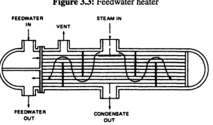
In large central station installation, from one up to a dozen of feedwater heaters are often used. These can attain length of over 60 ft., diameters up to 7 ft., and have over

30,000 ft.2 _{of surface. Figure 3.3 shows a straight condensing type of feedwater heater}

with steam entering at the center and flowing longitudinally, in a baffled path, on the out-side of the tubes. Vents are provided to prevent the buildup noncondensable gases in the heater, and are especially important where the pressures are less than atmospheric pres-sure. Also, deaerators are often used in conjunction with the feedwater heaters or as a sep-arate units to reduce the quantity of oxygen and other noncondensable gases in the feedwater heater to acceptable levels.

(26)

Figure 3.3: Feedwater heater FEEDWATER STEAM IN IN VENT I FEEDWATER _CONDENSATE OUT _OUT

3.1.2 Theoretical Development

The Extraction Steam Flow

The amount of the extraction steam flow is directly influenced by the thermodynamic process within the heater. Two important regulating mechanisms are the heat transfer pro-cess and the thermodynamic propro-cess. The heat transfer propro-cess occurs within the heater as well as between the heater and the environment. The thermodynamic process takes place within the control volume where upstream drain flow, heater drain flow, and extraction flow interact. The model used in predicting the extraction steam flow is based on the con-servation of energy, the concon-servation of mass, and the thermodynamic relations. The

model suggested by Davis is presented here. [5]

Figure 3.4: The control volume of the feedwater heater

Upstream Drain Flow Extraction Flow

Condenser Volume

(27)

1. Definitions of Variables

Vc = total volume of the condensing region

Mc = total mass of the water in the condenser

P = heater pressure

hf = saturated liquid specific enthalpy at P hg = saturated vapor specific enthalpy at P

hfg = hg-hf

hc = specific enthalpy of the condenser mixture

Vf _{= saturated liquid specific volume at P}

vg = saturated vapor specific volume at P

Vfg = Vg-Vf

vc = specific volume of condenser mixture

x = steam quality in the condenser

mI = extraction flow

h3 = specific enthalpy of flow from the desuperheater

m2 = upstream drain flow

h2 = upstream drain specific enthalpy

m5 = heater drain flow

h5 = heater drain specific enthalpy (assumed equal to hf)

UAco = UA for the heat transfer from condenser to tubes

LMTDco = condenser log mean temperature difference

UAhs = _{UA for the heat transfer from condenser to heat sink}

Ths = temperature of the heat sink

(28)

2. The Extraction Steam Flow Model

The conservation of mass states that

dMc V 3c = mi+m 2-m 5 where Mc = c. Vc Therefore, dM _{1 dVc Vcdvc} dt vcdt v2dt dV where

_dt

c = 0

since the condenser volume is constant. Now,

dM_c Vcdv_c

dt 2 dt = mi + m2 5 .

vC

Consider vc to be a function of the pressure and the enthalpy inside the condenser,

then

dvc

_v

dhc

dP

dt ,ahiJdt + ,(vh dh Derivation of d hc dt

The energy balance relation states that

d Mcuc = mIh3 + m2h2 - mh f - UAcoLMTDco + UAhs(Ths _- _{Tsat) .}

I +~ 2 mhfUCLT By definition, uc = hc - Pvc. Then, dt C = d M _(h -Pvc) = (hc-Pv dM) C+Mcdi(hc- Pvc) d dMc dMc dhA dP dv Mc= hccc -Pcc + + CcPdtc M cCcc -(3.1) (3.2) (3.3) (3.4) (3.5) (3.6) (3.7) (3.8)

(29)

Since Mcvc = Vc,

d dM dh dP ( dM + dvyc

dtM=u = h- h +M-dt -Vcd- -Py +Mc-i ).

However, since the condenser volume is constant,

dMc dvc d dVc Sc + M -M cvc = 0. Ct Cdt tC C d Hence, d dMc dhA dP dhc d dMC - Mcuc = hCdT + Mc -VdC t or m dt McUc - hcd +

VdP

Cdt •

Substitute the expression dMc in Eq. (3.5), we then have

dhc _dM _dP

Mcy- = mI h3 +m2h2 -m 5hf - UAcoLMTDco + UAhs(Ths- Tsat) -hc-dt + Vc •

Again, since

dMc t = ml

+m₂-m ₅, dh C 1_d_

dt - mI m(h3 - hc) +m2(h5(2hc)m(h _{hc) - UAcoLMTDco + UAhs} _hs _sat)+

h fg V c'

Derivation of Mh fg

Using the fact that

h

1

c = h•(V- Vf) + (hgvf- hfvg) and _{v-R = Vg- Vf,}

fg fg

v hg hf

vc = hch +V h _J _f_fg _ghf_h-.

By differentiating term by term,

hc Vfg hcfg fg h cvhfg ah _• -h2PC cfg h---g ) + (h -- ), (3.9) (3.10) (3.11) (3.12) (3.13) (3.14) (3.15) (3.16) (3.17)

(30)

hgvf(ahfg+ 4g ("gvf (hhgj

and

_' _{aPt.V -hf,}hv

hL

₎

=

hf g(ahfg.

I

h aVg ahf. h 2 W) hfg'faP gvgap j fg Therefore, ( = -h h -v By rearranging, By rearranging,

h

T2, (-DP

h

ap

fg gf fg A+ _{h+ vahf,.} (av = hc(hf Multiply by Mc,

hi

_A

₎

h fg hgvf )

Lf

_h

_{fg @ap,}aP Mc (cJ)h c = ch h-gs. ]2₁

)_

hL

(av.) h hfg (Ca'P -(hfvg hgvfh fg L( h fg g F

Note that the expressions in the bracket are single-valued functions of P.

The quality of the mixture x =

-Vfg

The enthalpy of the water in the condenser hc =h + .•) •f

Multiplying by Mc, we now have

Mchc = Mchf + ý! chfg Vfg M- vf •Ifg f Mc(hf - V fg fg + Vc hfg_fg" (3.18) Thus,

hMc

h

_hc

a

_z

_{_}

_/•

_h

(-a;Jh =c

I

fgjh f Vfg hfg + M[[(hfvg hgvfgh, hvf

Lf

hTP

f

htP

hf avg,_ vg, ahf"•

f•

fg

Further expanding the expression gives,

vhh

V g (Dh f)

h

f9 Vfahg ~]

V

f a

7g)

V_{f ahgn]}₁ hfg gP Vf1 ,ahg)]

h

a

J

a

A+

hI f" -av ahf.

hfg

(31)

F hf (J Vf (OVjg' hfVfg ah(,hg+ Vf (cJhjg ] Mc~) =Mc[Lj~t~j a -V j hV g~ fYP) c

rCh

_ vg A

pg

hng vf

_2h

ahfg+ h,

_ag

P

(a

_a)

f

_h

a gf

_P

vg (Jhf -

•g

;h

h

V

)j

+J -

f

+

+C_

Mct-•Jh = M_MIaI=MI ei CxM~ Lh vf v J'Vfg + fhjg Vfg ~3P + M h h +fvfg h + a hf~P Note that hf vg - h jVf +v fhfg = hf -h -hf(g - vf) + Vf(hg hf) = 0. Therefore, Mfc )h c hf V hjgP h a

Mctap Jh<. = Mc·lh • -V.~sgt.aP.h, ) ) hfgtvp i-P

-hNow, multiply the expression by

Now, multiply the expression by ,

MhgV

Vcg (a<ýh

_c) = hfghf Vf fI h v

-L- _fg\ _{+ v i-t}

_)f

CIfg h f VfA~ 3p-a)

+

f

+

+ V'[f

v (

aPfg

) hv

(A

f g

)]

gg\V ;gV _ v-g (Jhf V f9 P V f9 P V _{fD+ g} f9(( _a]hg __ II +vhfg [

vfV(gW

(nVfg

a;II]

fg

+

1 -1

This expression can alternatively be written in form of, Mi,-f h h

where A and B are strictly functions of pressure. From the original conservation of mass equation,

mi +m2-m5 - 2= +•JP)h.dt j

= McA + VcB ,

h M_ , [m,1 (h3 - hc) + m2(h - hc) - ms(h - hc) - UAcoLMTDco + UAhs(Ths - Tsat)]

VC f Vc (Vfg 1i dP Vc\ dP 2 7 hy Mc Cdt jP hdt

J

hg (~fa"•P

f9

I

mi+ m2 - m5

hf (cawg) vg (cahf +vfag

hj9*

h f9

fg P

(32)

Since vc=

-mi + m₂- ₅ = S[m (h3 - hc) + m2(h2 -hc) - ms(hf - hc) - UAcoLMTDco + UAhshs - Tsa

Vch f

fcLTc

e,(h

c

,,)

M fgdP

- Mg

chkdt

C

hcd '

h(-ml - m2 + 5) = ml (h3 - hc) + m2(h2 - hc) - m5(hf - hc) - UAcoLMTDco + UAhs(Ths - Tsat)

Vfg

dP Mch/fg(aVc dP

Cdt v fg P jhedt p i

Ultimately, the extraction steam flow can be expressed in the following form,

1

Vfg

h 1 3 - hc + v_Vfghfg

JMr2(h2 - hC - vchfg> rn5(hC - hf - vhgUA COLMTDCO + UAhs(Ths -

Tsd-Vfg / f (I hrh g a hf h h a gd Vfg hfg Vfg ~ _{"Vf+ý-'gCv)- f}Vfg Vfg

_{fg P-}

g Vfg

_(P

Vfg ~)JJ

_{T d}

Lv9

f fg W f9G hfgavfg Ih c v-•fg ( P Vgkr hP f )jdii

(33)

Fluid Flow Resistances

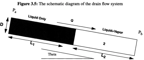
In this section, we will derive the dynamic model of the flow system from the drain

exit of the heater to the cascaded flow inlet of the downstream heater. Figure 3.5 shows the

schematic diagram of the system that our model is based on.

Figure 3.5: The schematic diagram of the drain flow system

Pa

1 J ...

2P ~ i +Vapr Pb

Theta

We will investigate both the case where the flow is assumed to be entirely single phase and the case where the flow downstream is in liquid-vapor phase. The flow through the drain valve is always in liquid phase. The pipe system is assumed to be well insulated therefore the heat transfer to the environment is negligible. The momentum flux changes due to the friction in the pipe is usually very small and is neglected in our model.

1. Single-Phase Flow

The pressure drop in the drain system occurs at two places. We will now consider the case which the flow is assumed to be entirely liquid. The pressure drop increases as the fluid passes further downstream through the drain pipe and the control valve.

Pressure Drop Across the Pipe

The equation which describe the pressure drop for a flow with velocity v is given by

AP = Kpv2 (3.19)

where the friction coefficient is defined as

(34)

K =

f

.

(3.20)

The friction factor, f, is a function of the relative roughness of the pipe and the Reynold's number. In the case which the flow is turbulence (Re > 2000),

f 0.316 (3.21)

Re0 2 5

By substituting the relation in Eq. (3.20)-(3.21) in Eq. (3.19) and solve for the pressure drop as a function of the volumetric flow rate Q,

Q = Av (3.22)

AP. = 0.316 rA0.25 Lp 2.

Apipe

=

_-[

_j

_L-

[

a

_I

_(3.23)

pipe Pressure Drop Across the Control Valve

The conventional equation for describing the relationship between the pressure drop and the volumetric flow rate is

S= c P, (3.24)

The valve coefficient, c,, is a function of the valve opening and is usually supplied by the valve manufacturer. We can then solve for the pressure drop across the valve as

APvalve = 3225.42 Q2 (3.25)

Cv

2. Two-Phase Flow

We are interested in modeling the effects of the two-phase flow particularly the flow mixture of liquid and vapor. Two-phase flow occurs quite frequently in the feedwater heater system. We are concerned with the downstream section of the drain pipe where the flow exits the valve and the pressure drops resulting in partial phase transformation from liquid to vapor. In this section, we will describe the method of characterizing the two-phase flow. However, it must be noted that despite a large number of studies related in this

(35)

area, there are many situations where the uncertainty can be as high as 50%. Most of the two-phase correlations are entirely empirical or semi-empirical. We will discuss the pre-diction of the static pressure gradient approximation along the straight pipe during the two-phase flow.

Frictional Pressure Gradient

In deriving the correlations, it is assumed that the homogeneous theory is applicable to the system of interest. The liquid-vapor mixture is treated as homogeneous with a density based on the assumption that both phases flow at the same velocity. This theory gives a reasonable result even in the case where the actual vapor velocity is as much as five times faster than that of the liquid. [4] Furthermore, it is assumed that both phases are in turbu-lent flow condition in a smooth pipe.

The two-phase component of the pressure gradient due to friction is described by

-Dp = DPFO (3.26)

where acpFLo is the two-phase multiplier and DpFLo is the pressure drop due to friction if the

flow were all liquid.

The Martinelli-Nelson correlation gives the following approximation for the two-phase multiplier

(2-n) (2-n)

2 _o

= 1+(F2 1) [x 2 (1-x) 2 +x(2-n) _(3.27)

where the Blasius exponent n and physical property parameter r2 _{are defined by}

log •LO)

n - -Go (3.28)

log

(ReGo

(36)

r2 _{= (L} _(3.29)

and the coefficient B is defined in the following table.

TABLE 1. Values of B for smooth pipes

r G(kg/m2s) B F 19.5 G 5 500 4.8 500 < G 5 1900 2400/G G > 1900 55/G0.5 9.5 5 F 28 G 5 600 520/(rG .5) G > 600 21/F F 2 28 15000/( F2G.5)

Friedel has shown that this table gives reasonable agreement with an extensive data bank [4]

XLO is the friction factor when the total mixture flows as liquid

XGO is the friction factor when the total mixture flows as vapor

Re is the Reynold's number

9G is the dynamic viscosity of the vapor phase

19

is the dynamic viscosity of the liquid phase

v is the specific volume

G is the mass velocity

Pressure Gradient due to Changes in the Elevation

Let the mixture density be p and e be the angle of the pipe to the horizontal line,

-Dpg = gpmsine (3.30)

Pm = apG + (1 -a)PL (3.31) Pressure Gradient due to Changes in Momentum Flux

The following equation describes the pressure drop in the straight pipe due to the change in momentum flux.

(37)

-DpM = G2 D(ve) _(3.32)

where

- = 1 + - 1 [Bx(1- x) + x2] _(3.33)

VL L

The derivative of ve can be expanded as

D(ve) [ Dp + [eDs (3.34)

Ds - D(q+F) _Dq DpFH (3.35)

T T T

where q is the heat transferred per unit mass and F is the frictional energy dissipation per unit mass. If we assume that the frictional energy and heat transfer is negligible in an insu-lated smooth pipe, the expression becomes

-Dpm = G2 P Dp = - Dp (3.36)

where Gc is the mass velocity at maximum flow condition (choked flow).

3.1.3 Kingston Unit 9 System Description

Kingston Unit 9 Feedwater Heater System

Kingston Unit 9 is a shell and tube heat exchanger in which the feedwater flows through the tube and interacts with the steam extracted from the turbine. As the heat from the extraction steam is transferred to the feedwater, some of it condenses and is collected at the bottom of the heater. The level of the water in the heater is critical to the efficiency of the heat transfer and must be controlled quite closely. If the level is too high, the feed-water tubes are submerged and the heat transfer decreases significantly. If the level is too low, the extraction steam in the shell could flow through the drain cooler and, because of its high velocity, can damage the tubes in that area. Moreover, the drain pipe is sized to

(38)

handle fluid not steam, so it will not pass adequate flow if the steam were to enter instead of water.

The level of the water in the shell is controlled by a control valve in the drain pipe. The water from the heater can flow to two different places. In normal condition, it will be passed to the next heater downstream where it is used to augment the temperature of the feedwater before it reaches the current heater. In emergency condition, the water will be passed through the emergency drain valve directly to the condenser of the main turbine. This is not desirable since it is not as efficient.

The heater level is currently controlled by a simple PI controller. There are a couple of system characteristics that can complicate the controller tuning. Ideally, the installed valve characteristic of the drain would be linear over the load range of the plant and the optimum controller gains would also be constant. However, this is not the case therefore the PI con-troller needs different gains over the load range for optimum response. The inherent valve characteristics should be selected to give the closest to liner response possible without any tweaking in the control system. The sizing of the drain pipe can also affect the flow char-acteristics quite significantly. These are the two factors which make it difficult to get a lin-ear installed valve characteristic (flow rate versus valve lift over the load range of the plant at actual differential pressure).

Hence, the current PI controller is tuned conservatively so that the stability is main-tained as the system characteristics change over the load range of the plant. If the mechan-ical system is well-designed, the performance is usually acceptable. The schematic of the feedwater heater diagram is given in Figure 3.6.

(39)

Figure 3.6: Kingston Unit 9 feedwater heater system schematic diagram

Kingston Unit 9 System Simulator

The Tennessee Valley Authority (TVA) Kingston Unit 9 simulator, constructed by Foxboro and ESSCOR, inc., is primarily intended as a training device for engineers and operators of Unit 9. The simulator teaches the trainees how to use the Foxboro I/A system under a variety of plant conditions such as start-ups, shut-down, and emergency situations. The simulator features an Instructor Station Package from which a supervisor can monitor a trainee's performance. Since the simulator exposes a trainee to a wide variety of operat-ing conditions and circumstances, the trainee may gather a lifetime of unit experience before ever operating the actual unit.

Another use of the simulator which is concerned with our operation is to test the effects of controls and/or plant modifications before implementing them on the actual unit allowing tuning optimization and early detection of flaws.

We will now define the terms simulator, model, and controls. The simulator is a com-plete combination of the Foxboro workstations, the master simulation computer loaded with all model and controls software, the instructor station, and all associated peripheral equipment. The model is the set of compiled and linked subroutines which simulates the behavior of the Kingston Unit 9 plant. Controls refers to the set of Foxboro unit 9 control

(40)

compounds and downloaded onto the master simulation computer from the Foxboro Applications Workstation.

1. Simulator Hardware

The control hardware portion of the simulator consists of three Foxboro consoles com-prised of one Applications Workstation (AW) and two Workstation Processors (WPs). The AW is the center console, flanked by the two WPs. Each workstation has a Sun Sparc LX as its processor.

The "plant" portion of the simulator consists of two Sun Microsystems workstations (a

Sparc 20 and a Sparc 5). The Sparc 20 has two machine names, kingmaster and SCP001.

It has two names since it must communicate not only with the Foxboro AW (to which it is

recognized by SCP001) but also the Sparc 5 (by kingmaster). These two names may be

used interchageably throughout this document. Kingmaster is the simulator "master"

com-puter on which the simulator model runs; it passes information to Sparc 5, which serves as

the Instructor Station. The machine name of the Sparc 5 is kingis. Figure 3.7 shows a

hardware block diagram of the simulator hardware. Machine names are in parenthesis and in bold.

SCP001(kingmaster) is connected to the Foxboro hardware through a Dual Node Bus interface (DNBI), and through a serial cable. The DNBI handles all communication between the CP and Foxboro controls, the serial cable passes CP "letterbug" information to the Hardware Connections portion of the Instructor Station.

(41)

Figure 3.7: Simulator hardware block diagram

I

ESSCOR .. Foxboro AW51(9AAW01) DNBI

II IVLvast4l II..-UtIV I I

Sun Sparc 5 Sun Sparc 20 1

(kingis) (kingmaster or SCP001)

WP51(9AWP01) "V

2. Simulator Software

The two key software elements of the Kingston unit 9 simulator are SYSL and FSIM. SYSL stands for System Simulation Language, and FSIM stands for Foxboro Simulation Language. The major functions of each are described below.

The Kingston Unit 9 plant is modeled using the combination of model subroutines and a SYSL input file. Each major plant sub-system (such as feedwater, air, fuel, etc.) is mod-eled in a FORTRAN subroutine. The SYSL input file forms the "backbone" of the model

by declaring all model variables used, and by making calls to the model subroutines. The

steps required to make an executable model are translation, compilation, and linking. When the model is translated, the SYSL input file is sorted so that the model subroutines

are called in proper order. The translation also converts the input file into compilable FORTRAN source code. This source code is then compiled and linked with the model subroutines, SYSL libraries, FSIM libraries, and engineering tool libraries. The result of this step is an executable model file. When the model is run, SYSL loops through the sorted list of model subroutines, updates variables accordingly, and increments the model timer to the next time step. The rate at which this is "marching" forward occurs can be controlled to make the model go faster or slower than the real (wall clock) time.

Ir nn I I

I

(42)

The SYSL modeling approach uses a combination of ordinary variables and state vari-ables. The ordinary variables are updated in the order in which they are called by the sorted SYSL input file. For example, if model variable a calculated in subroutine A is a function of model variable b calculated in subroutine B, SYSL will sort the input file such that subroutine B is called before A. State variables on the other hand are considered con-stant throughout the time step being calculated. These variables's derivatives are computed in the various model subroutines, but the state variables will only be updated (i.e. inte-grated) at the end of the time step, before proceeding to the next time step. The state vari-able approach to the modeling allows the greatest amount of modeling fidelity with the least consumption of computer processing time.

For the simulator to be useful, it must communicate with controls hardware in such a manner as to make the controls think it is "seeing" the real plant. FSIM accomplishes this task in two ways. First, running FSIM on the master simulation computer turns that com-puter into a "Soft Compound Processor" (hence, the kingmaster is also named SCP001). Second, FSIM provides the interface between the SYSL plant model and the controls soft-ware. This is accomplished through the use of an I/O Cross-Reference Table, in which controls compound:block.parameters are tied to SYSL model variables. Essentially, this cross reference table replaces the I/O cabinet and associated Field Bus Module hardware of a real plant installation. FSIM has a process called cio_cp, which synchronizes the con-trols processing with model processing. Since the model and concon-trols processing occur simultaneously, this process ensures that the model and controls run in "lock-step".

3.1.4 Transient Response Data Acquisition

Closed-loop Tests From Kingston Unit 9 Plant

The purpose of conducting the field tests is to use the result to compare with the simu-lator's model predictions. Heater #1 was subjected to level setpoint changes around the

(43)

nominal value of 8 inches with the magnitude of 1 inch or greater. Only the closed-loop tests were conducted since the plant operators suggested that the heater emergency dump valve might be triggered if the control loop were opened. Such condition will be undesir-able since the actual plant efficiency will decrease and the level recorded will be the result of the combined effect of the drain valve and the unmodelled emergency dump valve.

Eight signals from heater #1 were recorded. However, we are most concerned with the heater #1 level and the heater #1 valve command. As we have mentioned earlier in the the-sis, the level controller used in the feedwater heater at Kingston Unit 9 is proportional plus integral type where both gains can be varied on-line. Three sets of gains were used in the

tests with [PB = 35 ; INT = 1.7] being the set which is commonly used.

TABLE 2. Kingston Unit 9 closed-loop response tests

Test Number Proportional Band Integral Time Setpoint Command (in)

1 35 1.7 8.0-9.0-8.0

2 25 1.7 8.0-9.0-8.0

(44)

(45)

'B = 25 NT = 1.7 O: 98:OO 18:57 91 S 7.98S5 4.5661 5. 6113 0.0144 Inch.. Inches inches Inehes Bi 62 PAl 'a

IT

.

T

.

9f

E

Iu

m

IIImi

I...II

f

1 II

--A JAL,

_OR7

I rP...H RS IT_{PHT it S}

feoe

T

P. HTs

_tROR

HT 1!8 I I.98 0" O : 18: 57 e1 5 47.4, 9.09 29.468 -0,5661 % Ole9 YH I gBS TRS

T,

. 9 P..HT!!t I1T .OO HPHTRS I

.ee

IP- HTRS ROR 1, 6OeO

i

9-84

ER

I'iii"u .•uni ,l- ni.mu•, - • i; 1 - Iii ...._I

-- -- ~ -~-

----I I i I I I I ~· i ~C I I I I I I' r ~---- -n---luL

: - ~" - 1----;~- --- ---- ~~~- : --

:-;---~- ~- --~a I -- ,-,,_,-, - ~-r--- - -II - cL~--~~--~-·-~S I

(46)

PB= 18 INT = 1.7 BBrggs:19 77 a

ki·

71'

-A44

-· - ---·· i i _r -- ·- --i: --' iai~ ,.".°,i_*,4'7.. .3 •:.. ₄₃₁₈ 5 1e*Es

Li~

.1 S 7.9443 4. 12 43 S .7 5 3 0.90352

-I

o aches i n ocheo 32_PI 4'

5.

31 _P.

EI IP.HTRS IT IP.HTRS I.tor S go , .sees lb.: *gt 14 ? iI . Ol. 2. a.' ,rMP 'BUT : yg' .: i---· ~rl~i··i3~ ; i .... · .~ S i L ·

VVi

wv

--PrarroPe

::

:.:..

.: ....

; ...

I· :; ::

:: :;·

::

''

"If

as,

- _IU'tie

so.

3.. 34

I,

9.: _. lIT IS 000 - -- - 1. -~.-~. ~I___.,~ . Ilr'

kA

"" -I ·. --- ·- -Rb~ar --.. .. . . ... .. .... .. . .. . . •.l ... -~' -~--1 ~0161~86~~ ~;~i~4~i~i~B :n -:i·. re

cap

AAAA,

- -••••v: i ..i .. • .. . ---- ---- · - I ---~rr*r --- ~ _9· · ;-Y~q~~ ~16 -- -- ----· i· ;·. JI~C~F~~_{~-· ·}

m•

... i • . . .. . . rrrYra ~I st

pb;s~;i~;i

_{_~}

_:.::

_~...,

·?i: · ~;· Illr 9i 5' 1 I II " : " ' i

1OWN("

... . .. .. . --·~ ·: i ~ci i: i: : ·- · · :· ---· ;· :j;· r i ---- ·- --· --·---· i __ : i -- --LAA

~

ERR

milli

i;

I

I ~ -· -·I I r~ iI - --- ~--- r-~~~~~~~~~~~-r··· · · ·- r~~~r---rr"i`i~i;~c;:l-c-i--·~·-;II ~Li-l~~'-rr'·bir*-"'Lr~ i: [•; :-!7 • - ,i•..!i• * •.::o. .o

(47)

Closed-loop Tests From Kingston Unit 9 Simulator System

A number of similar transient response tests were also conducted on the plant

simula-tor to verify that the simulasimula-tor model gives reasonably accurate predictions of Kingston Unit 9 feedwater heater system. Throughout the tests, the same proportional plus integral controller was used on the simulator. The gains were changed at the simulator's operator station each time a new test was conducted. Table 3 described the conditions in which each test was carried out.

TABLE 3. Simulator closed-loop response tests

Test Number Proportional Band Integral Time Setpoint Command (in)

1 35 1.7 8.0-9.0-8.0

2 25 1.7 8.0-9.0-8.0

(48)

Figure 3.11: Simulator closed-loop test 1

Conventional PI controller with PB = 35 and INT = 1.7

I I I i I I I

I

0 100 200 300 400 500 600 700 800 900 time (s) 0 01 I 0 0 100 200 E 22 S20 U) 1 18 u_ LL 195 194 Z 193 03 300 400 500 600 700 800 900 time (s) I I I I . I I I 0 100 200 300 400 500 600 700 800 900 time (s) - · . . . . . . . . . . . . . . . . . . . . . . .. . . . . . ... . . 0 100 200 300 400 500 600 700 800 900 time (s) A .G 1 oo I LL .--I 8 6 8 .. . .. . · · ·

...

I I I I I I I . I

(49)

Conventional PI controller with PB = 25 and INT = 1.7

20 40 I I8 0 200 400 600 800 1000 time (s)

> 0 .5

...

LL 0 0 0 200 400 600 time (s) 800 C,, time (s) - 195--z 193 0c 0 200 400 600 800 time (s) A I 8 - 1 cl) I_ LL 6 o • - 1 1000 1000 0 Ov

(50)

Conventional PI controller with PB = 18 and INT = 1.7 8I

8

0 I I I I I 200 400 600 800 1000 time (s) I . . N.I 0 200 400 600 time (s) 800 4, r- 0% time (s) 195 194 _.,_., _I ._i _, _i 200 400 600 time (s) 800 0 '-1 U') I U._ -j SO_,- ₁ > 0.5 _O"

. ...

1

1000 z I D3 1000 '-L" ' ' "

i

I

... time (s) I_... I• . . . .. . . . . . . . . . . ...

(51)

3.1.5 Summary and Remarks

TABLE 4. Transient response results from Kingston Unit 9 plant

Test PB INT Setpoint Overshoot Settling Time

1 35 1.7 8.0-9.0-8.0 - 10% -40s

2 25 1.7 8.0-9.0-8.0 - 5% -30s

3 18 1.7 8.0-9.0-8.0 - 5% -25s

TABLE 5. Transient results from Kingston Unit 9 simulator

Test PB INT Setpoint Overshoot Settling Time

1 35 1.7 8.0-9.0-8.0 < 2% 48s

2 25 1.7 8.0-9.0-8.0 < 2% 37s

3 18 1.7 8.0-9.0-8.0 < 2% 28s

The tables above summarize the closed-loop transient response tests result for both the actual feedwater heater system and the simulator. It is noted that due to the graphical nature of the field information obtained from the actual system, only approximates of the overshoot and the settling time can be realized. It is not uncommon that there is a subtle difference in the overshoot characteristics since the simulator cannot capture all the pre-vailing heater dynamics especially those of higher orders. However, the magnitude of the settling time in both cases are quite similar.

The tests result states that we have the error interval of about 20 percents for the set-tling time and slightly higher for the percent overshoot. With careful considerations, we can then use the simulator as the test bed for our new controllers and assume that the tran-sient response result will be within reasonable range of the actual system.

Applications of adaptive controllers based on nonlinear parametrization to level control of feedwater heater and position control of magnetic bearing systems

Applications of Adaptive Controllers Based on

Nonlinear Parametrization to Level Control of

Feedwater Heater and Position Control of

Magnetic Bearing Systems

by

Chayakorn Thanomsat

B.S., Mechanical Engineering

Carnegie Mellon University (1995)

Submitted to the Department of Mechanical Engineering

in partial fulfillment of the requirements for the degree of

Master of Science

at the

MASSACHUSETTS INSTITUTE OF TECHNOLOGY

May 1997

@ Massachusetts Institute of Technology, 1997. All Rights Reserved.

A

uthor ...

...

Department of Mechanical Engineering

May 9, 1997

Certified by ...

...

...

Anuradha M. Annaswamy

Associate Professor of Mechanical Engineering

Thesis Supervisor

A ccepted by ...

Ain A. Sonin

Chairman, Department Graduate Committee

Applications of Adaptive Controllers Based on

Nonlinear Parametrization to Level Control of

Feedwater Heater and Position Control of

Magnetic Bearing Systems

Abstract

Acknowledgments

Table of Contents

List of Figures

List of Tables

Chapter 1

Introduction

1.1 Motivation and Contribution of Thesis

1.2 Synopsis of Thesis

Chapter 2

Adaptive Controller Based on Nonlinear

Parame-trization

2.1 Introduction

2.2

The Adaptive Controller

2.2.1 Problem Statement

2.2.2 The Controller

(2.13)

-

2.2.3 Extensions

Chapter 3

Level Control in Feedwater Heater System

3.1 Preliminaries

3.1.1 Introduction

The Rankine Cycle

The Regenerative Cycle

3.1.2 Theoretical Development

The Extraction Steam Flow

dt

dvc

dhc

dP

VdP

h

1

and

hL

=

I

h

h

ap

hi

A

)

Lf

_dt

_A

₎

_h

_hc

_z

_{_}

_h

_2h

_ag

_a)

_h

_P

_)f

hj9*

_{fg P-}