HAL Id: hal-02196117
https://hal.archives-ouvertes.fr/hal-02196117
Submitted on 2 Jul 2020
HAL is a multi-disciplinary open access
archive for the deposit and dissemination of
sci-entific research documents, whether they are
pub-lished or not. The documents may come from
teaching and research institutions in France or
abroad, or from public or private research centers.
L’archive ouverte pluridisciplinaire HAL, est
destinée au dépôt et à la diffusion de documents
scientifiques de niveau recherche, publiés ou non,
émanant des établissements d’enseignement et de
recherche français ou étrangers, des laboratoires
publics ou privés.
K. Juhel, Jean-Paul Ampuero, M. Barsuglia, P Bernard, P Chassande-mottin,
P. Fiorucci, J. Harms, J. Montagner, Martin Vallée, P Whiting
To cite this version:
K. Juhel, Jean-Paul Ampuero, M. Barsuglia, P Bernard, P Chassande-mottin, et al.. Earthquake
early warning using future generation gravity strainmeters. Journal of Geophysical Research : Solid
Earth, American Geophysical Union, 2018, 123 (12), pp.10889-10902. �10.1029/2018JB016698�.
�hal-02196117�
Earthquake Early Warning Using Future Generation Gravity
Strainmeters
K. Juhel1,2 , J. P. Ampuero3 , M. Barsuglia1, P. Bernard2 , E. Chassande-Mottin1, D. Fiorucci1,
J. Harms4,5 , J.-P. Montagner2 , M. Vallée2 , and B. F. Whiting6
1AstroParticule et Cosmologie, Université Sorbonne Paris Cité, Paris, France,2Institut de Physique du Globe de Paris, Université Sorbonne Paris Cité, Paris, France,3Université Côte d’Azur, IRD, CNRS, Observatoire de la Côte d’Azur, Géoazur, Sophia Antipolis, France,4Gran Sasso Science Institute, L’Aquila, Italy,5INFN, Laboratori Nazionali del Gran Sasso, Assergi, Italy,6Department of Physics, University of Florida, Gainesville, FL, USA
Abstract
Recent studies reported the observation of prompt elastogravity signals during the 2011 M9.1 Tohoku earthquake, recorded with broadband seismometers and gravimeter between the rupture onset and the arrival of the seismic waves. Here we show that to extend the range of magnitudes over which the gravity perturbations can be observed and reduce the time needed for their detection, high-precision gravity strainmeters under development could be used, such as torsion bars, superconductinggradiometers, or strainmeters based on atom interferometers. These instruments measure the differential gravitational acceleration between two seismically isolated test masses and are initially designed to observe gravitational waves around 0.1 Hz. Our analysis involves simulations of the expected gravity strain signals generated by fault rupture, based on an analytical model of gravity perturbations in a homogeneous half-space. We show that future gravity strainmeters should be able to detect prompt gravity perturbations induced by earthquakes larger than M7, up to 1,000 km from the earthquake centroid within P waves travel time and up to 120 km within the first 10 s of rupture onset, provided a sensitivity in gravity strain of 10−15Hz−1∕2at 0.1 Hz can be achieved. Our results further suggest that, in comparison to conventional
P wave-based earthquake-early warning systems, gravity-based earthquake-early warning systems could
perform faster detections of large offshore subduction earthquakes (at least larger than M7.3). Gravity strainmeters could also perform earlier magnitude estimates, within the duration of the fault rupture, and therefore complement current tsunami warning systems.
1. Introduction
During an earthquake rupture, fault slip and the propagation of seismic waves redistribute masses within the Earth. The mass redistribution generates a dynamic long-range perturbation of the Earth’s gravity, which propagates at speed of light and is thus recordable before the arrival of the direct seismic waves (Harms et al., 2015; Montagner et al., 2016; Vallée et al., 2017). These prompt gravity perturbations have been observed with broadband seismometers and superconducting gravimeter during the M9.1 Tohoku-oki earthquake (Montagner et al., 2016; Vallée et al., 2017). The potential contribution of such signals to tsunami early warn-ing is substantial: such observations would indeed have provided an early estimate of a magnitude greater than M9 within 3 min of the earthquake origin time.
However, two factors hinder the observation of prompt elastogravity signals with ground-based seismome-ters: the background seismic noise and a partial cancellation between the gravitational perturbation and its induced ground acceleration, whose difference is recorded by the instruments (Heaton, 2017; Juhel et al., 2018; Vallée et al., 2017). Elastogravity signal detection based on individual seismometer records is thus limited to earthquakes with magnitudes larger than 8.
One approach to improve earthquake monitoring capabilities is to overcome the limitations associated with the use of ground-coupled seismometers and gravimeters, by measuring the differential gravitational accel-eration between two seismically isolated test masses. This detector concept is known as a gravity strainmeter. Gravity strainmeters designed to observe signals at 0.1 Hz, within the frequency range needed to detect earthquake-related gravity changes, are being developed for gravitational waves (GW) sources detection in the subhertz domain (Harms et al., 2013) and are briefly reviewed in section 2. We note that the subhertz
RESEARCH ARTICLE
10.1029/2018JB016698
Key Points:
• Future high-precision gravity strainmeters could record prompt gravity signals before the seismic waves arrival during an earthquake rupture
• Planned sensitivity is sufficient to observe gravity perturbations from earthquakes of magnitude larger than 7 at distances up to 1,000 km • Gravity-based warning system
could perform faster detection and magnitude estimation of large earthquakes compared to conventional systems Supporting Information: • Supporting Information S1 Correspondence to: K. Juhel, [email protected] Citation:
Juhel, K., Ampuero, J.-P., Barsuglia, M., Bernard, P., Chassande-Mottin, E., Fiorucci, D., et al. (2018). Earthquake early warning using future generation gravity strainmeters. Journal
of Geophysical Research: Solid Earth, 123, 10,889–10,902.
https://doi.org/10.1029/2018JB016698
Received 12 SEP 2018 Accepted 1 DEC 2018
Accepted article online 8 DEC 2018 Published online 21 DEC 2018
©2018. American Geophysical Union. All Rights Reserved.
instruments are much smaller, lighter than the instruments developed for high-frequency (>100 Hz) GW detection (1-m scale compared to 1-km scale). Moreover, GW detection has very stringent requirements; thus, the sensitivity needed for earthquake detection should be achieved at an earlier stage of the instrument devel-opment. In contrast to seismometers, gravity strainmeters implement sophisticated seismic isolation schemes to measure differential displacements or rotations between test masses. The differential measurement rejects partially the background seismic noise and the gravity-induced inertial acceleration, which are similar for the two masses. Thus, for measuring earthquake-induced gravity perturbations, gravity strainmeters may be considered as a natural step toward improved sensitivities.
In section 3, we assess the detectability of prompt gravity strain perturbations generated by fault ruptures. We show that gravity strainmeters at planned sensitivity (10−15Hz−1∕2at 0.1 Hz) should be able to detect
earthquakes larger than M7 up to 1,000 km from the epicenter within P wave travel time and up to 120 km within 10 s of the rupture onset. For instance, a network of around 10 of these gravity strainmeters deployed every 200 km along the western U.S. coast should be able to monitor the onset of earthquakes down to M7 in the California-Washington corridor. On the other hand, a network of gravity strainmeters deployed further away inland (say 500 to 1,200 km from the coasts) should be able to monitor the overall rupture of the largest events and evaluate their final moment.
In section 4, we further evaluate quantitatively the improvement of earthquake early warning systems (EEWS) that could be obtained, in principle, by using the gravity strainmeters under development. Current EEWS are automatic systems formed by seismometers and communication networks, intended to detect the occurrence of an earthquake before the arrival of ground-shaking waves and to disseminate the information to the popu-lation (Allen et al., 2009; Heaton, 1985). Conventional EEWS rely on detecting the seismic P waves, which travel at several kilometers per second and are roughly twice as fast as the usually stronger, more damaging S waves. The finite speed of seismic waves, along with the density of a seismic network, signal transmission delays, the minimal number of stations, and signal duration required to estimate earthquake magnitude impose together a minimum on the warning time. Since changes in gravity propagate at the speed of light, a gravity-based warning system could give a potential gain in the warning times with respect to conventional EEWS. Every saved second can have an important impact in terms of life preservation and earthquake mitigation, since advanced warning enables the launching of automatic prevention systems and the implementation of safety procedures (Allen, 2013). We show that a gravity-based warning system could perform faster detections of large offshore subduction earthquakes and early magnitude estimates, available as soon as the rupture stops.
2. High-Precision Gravity Strainmeters
2.1. Detector Concepts
Gravity strainmeters are instruments designed to measure components of the gravity strain tensor h, which is the second time integral of the spatial gradient of perturbed gravity acceleration𝛿g:
h(r, t) = ∫ t 0 ∫ 𝜏′ 0 𝛁𝛿g(r, 𝜏) d𝜏d𝜏′. (1)
Very sensitive gravity strainmeters have been developed in the context of GW detection. In their advanced configurations, laser-interferometric GW detectors LIGO (Abbott et al., 2009) and Virgo (Accadia et al., 2011) have designed strain sensitivities of 10−23Hz−1∕2between about 30 and 2,000 Hz. Due to their poor
sensi-tivity in the subhertz region, advanced GW detectors cannot be used to measure gravity perturbations from earthquakes. In fact, in order to produce noticeable terrestrial gravity noises in the sensitive frequency band of advanced detectors, it has been shown that typical density perturbations have to be generated very close to the suspended test masses, that is, within a few tens of meters (Driggers et al., 2012; Harms et al., 2009). This means that terrestrial gravity perturbations that will be measured in advanced detectors are likely to be of little interest in geophysics.
To access the subhertz region, which is very rich in GW sources (Harms et al., 2013), three concepts for 0.1-Hz gravity gradiometers are currently under development: superconducting gradiometers (SGG) (Moody et al., 2002; Paik et al., 2016), torsion-bar antennas (e.g., TOBA; Ando et al., 2010, or TorPeDO; McManus et al., 2017), and atom-interferometric gradiometers (Geiger, 2017; Hohensee et al., 2011). In the following, we will refer to these detectors as GG10, that is, gravity gradiometers with high-sensitivity for signals with periods around 10 s.
All three concepts present novel solutions to the mitigation of seismic noise, which would otherwise exceed gravity signals by many orders of magnitude. The superconducting gradiometer achieves seismic-noise reduction by common-mode rejection in the differential readout of test-mass positions relative to a common, stiff reference frame. Torsion-bar antennas can be engineered with very low torsion resonance frequency, which constitutes an efficient passive filter of rotational seismic displacement. The rejection of translational displacement noise is obtained by reading-out the differential signal from two suspended bars (or a bar with respect to a suspended platform; Shimoda et al., 2018). Atom-interferometric gradiometers read out the dis-placement between freely falling ultracold atom clouds, which also provides partial immunity to seismic noise. In order to reduce the requirements of the seismic rejection, additional passive or active seismic-isolation techniques can be used (Winterflood, 2001).
The most sensitive instrument so far is the superconducting gradiometer with a strain sensitivity of about 10−10Hz−1∕2at 0.1 Hz (Moody et al., 2002). However, extensive gain in experience with these technologies
has led to defining more ambitious strain-sensitivity targets: 10−15Hz−1∕2at 0.1 Hz (Ando et al., 2010; Hogan
et al., 2011; Hohensee et al., 2011). It will be shown in section 3.2 that such design sensitivities are sufficient for the detection of prompt gravity perturbations from earthquakes (of magnitude> M6.5). It should be noted that all three concepts are also being considered as candidates for future, subhertz GW detectors with more ambitious sensitivity targets (10−20Hz−1∕2at 0.1 Hz; Harms et al., 2013; Paik et al., 2016).
2.2. Detector Sensitivity Models
The response of different types of gravity strainmeters to gravity-gradient fluctuations is not identical (Harms, 2015). The consequence is that instrumental noise spectra differ qualitatively between detector types. Current experimental efforts for all prototypes have the common gravity-strain sensitivity target of about 10−15Hz−1∕2
at 0.1 Hz. Below 0.1 Hz, instrumental noise in all concepts rises steeply. The high-frequency noise spectra dif-fer more strongly. While it is expected that instrumental noise of the superconducting gradiometer keeps falling above 0.1 Hz (in units of gravity strain; Moody et al., 2002), torsion-bar antennas have a flat noise spec-trum above 0.1 Hz (Shoda et al., 2014), and atom-interferometric gradiometers reach their best sensitivity only within small frequency bands (Cheinet et al., 2008).
For the purpose of this paper, we will use simplified sensitivity models to represent all GG10 concepts. The simplified approach chosen here is to assume that the sensitivity is proportional to 1∕f2at low
frequen-cies, that signal contributions below 0.01 Hz are not considered (GG10 detectors are not designed for such low-frequency observations), and that instrumental noise at high frequencies is frequency-independent. To estimate the detection horizon of gravity strainmeters to earthquakes, four sensitivity models are tested: flat strain sensitivity of 10−15Hz−1∕2above 0.05 and 0.1 Hz (models 1 and 2, respectively), 10−14Hz−1∕2above
0.05 Hz (model 3), and 5 × 10⁻¹⁷Hz−1∕2above 0.5 Hz (model 4). The resulting sensitivity curves are shown in
Figure 1, along with TOBA Phase III and SGG sensitivity curves. For the SGG sensitivity curve, a 20-kg mass and a 2-m-long baseline are used, along with an energy resolution EAof the superconducting quantum-interference device 10 times better than current commercial DC superconducting quantum-interference device values (Griggs et al., 2017).
2.3. LGN
GG10 detectors have different limiting noise sources and experimental challenges to reach the target of 10−15Hz−1∕2at 0.1 Hz, specific to each detector. A detailed description of the contributions of various noise
sources to the target sensitivity and the techniques to reduce them can be found in the references for each detector. But a gravity noise foreground is common to all the detectors: the local gravity noise (LGN). The LGN has several contributions: seismic LGN produced by density changes in the ground due to seismic waves; atmospheric LGN generated by density fluctuations in the atmosphere due to, for instance, infrasounds, tem-perature changes, and turbulences; and LGN associated with human activity (Harms, 2015). This noise couples with the detector in a way completely equivalent to the earthquake signal: it is then impossible to shield the detector from it.
Provided that the detector is located at a sufficiently remote site to avoid transient contributions to gravity as could be produced by cars or trucks passing close to the detector, the LGN contributions that need to be mit-igated further are of seismic and atmospheric origin. One way to mitigate the LGN is to select seismically and atmospherically quiet sites. To some extent, this can be achieved by constructing the detector underground, but since seismic and sound waves have long wavelengths around 0.1 Hz, the associated gravity disturbances are only weakly suppressed underground for feasible detector depths (Beker et al., 2011; Fiorucci et al., 2018).
Figure 1. Simplified sensitivity models for gravity gradiometers designed for high sensitivity around 10 s, along with
TOBA Phase III and SGG sensitivity curves. Several noisefloors (10−14,10−15, and5 × 10−17Hz−1∕2) and corner frequencies (0.05, 0.1, and 0.5 Hz) are considered to estimate the detection horizon of future gravity gradiometers to earthquake ruptures. SGG = superconducting gradiometers; TOBA = torsion-bar antennas.
As an alternative solution to LGN mitigation, it was proposed to coherently subtract LGN using data from arrays of environmental sensors, such as seismometers for the seismic LGN and microphones for the infrasound atmospheric LGN (Cella, 2000; Harms & Paik, 2015). The idea is to obtain sufficient information about local mass-density fluctuations to calculate an accurate estimate of the associated LGN. This method exploits cor-relations between environmental sensors and the GG10 detector by calculating a Wiener filter whose output corresponds to the optimal (linear) estimate of the LGN (Driggers et al., 2012).
Based on models for the infrasound atmospheric LGN from Fiorucci et al. (2018) and the even smaller seis-mic LGN (see for instance Figure 9 from ; Harms et al., 2013), we note that above a few millihertz, these LGN components should not affect significantly the GG10 sensitivity required for the earthquake-related signal detection. This will be shown in section 3.2. Nevertheless, we point out that the use of average seismic and infrasound spectra to estimate the LGN components can lead to underestimate the challenge associated with this noise. With this in mind, while work is ongoing to reduce further these noise contributions, it is assumed for the remainder of the paper that all forms of x lie below the instrumental noise at all frequencies.
3. Detectability of Prompt Gravity Strain Perturbations
3.1. Optimal Matched-Filter Detection and SNR
In order to assess the detectability of the gravity perturbation, we compute the signal-to-noise ratio (SNR) obtained with each gravity strainmeter described in section 2.2. To compute the SNR, we consider detection via optimal matched filtering (Jaranowski & Królak, 2012), which is based on the cross correlation between the gravity data and a template of the expected gravity strain perturbation. Template-matching techniques have been widely used in modern seismology to detect earthquakes with low SNRs (Frank et al., 2014; Gibbons & Ringdal, 2006; Shelly et al., 2007) and in astrophysics to detect coalescing compact binaries (Bose et al., 2011; Pai et al., 2001).
For simplicity, the detector noise is here assumed to be Gaussian and stationary. Before the matched filter is applied, both the template and the detector data are passed through a whitening filter, in order to obtain an approximately frequency-independent detector noise spectral density. The whitening filter is a highpass filter (Butterworth, two poles) whose corner frequency is the corner frequency of the considered instrument sensitivity model. Once the noise spectrum is uniformly distributed, the optimum filter is the time-reversed,
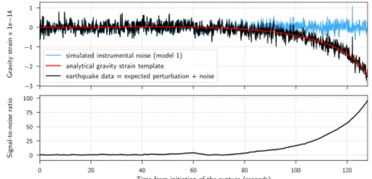
Figure 2. Earthquake data and signal-to-noise ratio time series during a
M7.5 earthquake. (top) Whitened gravity strain data (black curve,hEZ component) recorded by a model-1 gravity strainmeter located 1,000 km away from the epicenter of a M7.5 dip-slip earthquake. The recorded data are obtained as the sum of the whitened instrumental noise (blue curve) and the whitened gravity strain template (red curve; Harms, 2016). (bottom) Corresponding signal-to-noise ratio, defined as the ratio between the data filtered with the time-reversed template, and the standard deviation of the noise filtered with the time-reversed template. The time series are truncated at P wave arrival time, 128 s after the earthquake onset time.
whitened template. The SNR is then defined as the ratio between the output of the optimal matched filter in the presence of a signal and the standard deviation of the output in the absence of a signal.
3.2. SNR at P wave Arrival Time and 10 s After Onset Time
In order to compute the gravity signal templates for a class of earthquakes, a model for source time functions (STF) should be used. In this section we adopt a self-similar source model, which implies that the initial phase of a large-magnitude event is identical to that of a lower-magnitude event. While this universal rupture-initiation behavior is still debated (Colombelli et al., 2014; Meier et al., 2016, 2017), such hypothesis is a classic assump-tion and represents the worst-case scenario for EEW. Here the following self-similar model of seismic moment rate function ̇M0is employed:
̇M0(t) = a M0 T (t∕T) 2 (2) if 0< t < T , and ̇M0(t) = a M0 T ( 1 − (t∕T − 1)2)6 (3) if T < t < 2T , where T is the half-duration of the rupture and a a scalar. We adopt the empirical magnitude-duration relation 2T = (M0∕ 1016N.m)1∕3(Houston, 2001). The shape of the first half of this source
time function is that of a circular crack with constant rupture speed and uniform stress drop. The second half is a polynomial approximation to the stopping stage in the moment rate function of the circular crack model of Madariaga (1976).
Based on this source model, we compute gravity strain perturbations for various magnitude-distance pairs, induced by a dip-slip event with angles (strike, dip, rake) = (180∘, 10∘, 90∘). We consider magnitudes ranging from 5 to 9.1 and epicentral distances ranging from 75 to 1,100 km. Ten different azimuths are considered, ranging from 270∘ to 360∘ such that half of the down-dip part of the radiation pattern is computed (the remaining half being inferred by symmetry).
We first compute vertical (Z) gravity perturbations𝛿gzin a half-space model, using the analytical formulations developed by Harms (2016). The medium is defined by a P wave velocity of 7.8 km/s and an S wave velocity of 4.4 km/s, such that the P wave arrival times for stations located 250 to 1,100 km away from the epicenter are globally comparable to travel times obtained in a more realistic Earth model, such as the Preliminary Reference Earth Model (PREM) (Dziewonski & Anderson, 1981). The (EZ) and (NZ) components of the gravity gradient tensor𝛁𝛿gzare then obtained by the finite difference of gravity perturbations𝛿gzcomputed at two close locations, aligned along the East-West (E-) and North-South (N-) directions. Two integrations over time then lead to the associated gravity strain perturbations hEZand hNZ.
We add simulated instrumental noises, for the four different sensitivity models considered in section 2.2. For each magnitude and distance, we then apply the optimal matched filter (i.e., the whitened template used to compute the synthetic earthquake data) with a finite duration time window and normalize by the standard deviation of the matched-filter output in the absence of signal. The result is a set of continuous time series of SNRs, with values fluctuating around 1 during the absence of a signal. An example of hEZgravity strain data and corresponding SNR time series are shown in Figure 2, for a model-1 gravity strainmeter located 1,000 km away from the epicenter of a magnitude M7.5 earthquake, in the along-dip direction. At P wave arrival time, 128 s after the earthquake onset time, the SNR reaches ∼100.
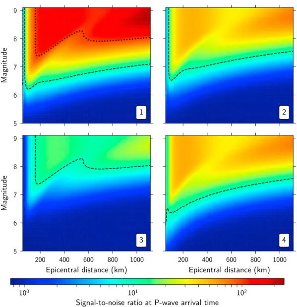
For each epicentral distance and magnitude, the SNRs accumulated within the travel time of P waves to the detector are shown in Figure 3. Each point of the contour plot is the average SNR obtained for 10 different azimuths, two components of the gravity strain tensor (hEZand hNZ), and a hundred different realizations of the detector noise. As expected, SNRs globally increase with increasing magnitudes. Two lobes of high SNRs are observed at high magnitudes, separated by a region of lower SNR where the gravity strain records reach
Figure 3. Signal-to-noise ratio accumulated within P wave travel time to the detector as a function of event magnitude
and distance of the detector. The sensitivity models 1 to 4 of the next-stage gravity strainmeter are used (see section 2.2). Contour lines are for signal-to-noise ratio = 10 (dashed) and 100 (dotted).
a zero crossing at P wave arrival time. The zero crossing is observed at longer epicentral distances for higher magnitudes, since higher magnitudes are associated to STF with longer half-duration (which acts as a low-pass filter on the gravity strain record). High SNRs (>50) are reached within P wave travel times for detector models with high-sensitivity around 0.1 Hz (models 1, 2, and 4). The highest ratios (>100) are measured with the model-1 sensor, which displays the highest sensitivity at low frequencies. For this model, SNRs larger than 10 are reached for every earthquake of magnitude larger than 7, up to 1,000 km from the epicenter. An improved high-frequency sensitivity (from model 2 to model 4) leads to slightly higher SNRs for epicentral distances below 300 km.
The SNRs of signals measured within the first 10 s of a fault rupture are shown in Figure 4. The SNRs increase with decreasing epicentral distances and saturate for event magnitudes greater than 6.5 as a consequence of self-similarity (the moment rate functions of earthquakes of larger magnitudes are identical in the ini-tial 10 s). Accordingly, earthquake detection with SNR higher than 10 based on only 10 s of data would require next-stage detectors to be about 100 km or closer to the hypocenter, independent of the event mag-nitude above M6.5 (models 1 and 4). Improved low-frequency sensitivity (from model 2 to model 1) and high-frequency sensitivity (from model 2 to model 4) lead to improved SNRs.
Figure 4. Signal-to-noise ratio accumulated within the first 10 s after onset time, as a function of event magnitude and
distance of the detector. The sensitivity models 1 to 4 of the next-stage gravity strainmeter are used (see section 2.2). Contour lines are for signal-to-noise ratio = 5 (dashed) and 10 (dotted).
While the detector corresponding to sensitivity model 3 (10−14Hz−1∕2above 0.1 Hz) should detect events
of magnitude M7.5 and above with SNR higher than 10 at P wave arrival time (see Figure 3), its use for EEW purposes appears to be limited (see Figure 4). Prompt detections of earthquake-induced perturbations thus require the strain sensitivity target of 10−15Hz−1∕2at 0.1 Hz.
The circular crack model assumed in this section may be inappropriate for earthquakes of magnitude larger than M7. Indeed, large ruptures transition from circular to an elongated shape if they saturate the along-dip width of the seismogenic zone. Once the circular assumption breaks down, the t2moment-rate growth of
equation (2) slows down to t1if slip scales with rupture length (L-model, Scholz, 1982) or t0if slip scales with
rupture width (W-model, Rundle, 1989). With the fault dip (10∘) and hypocenter depth (20 km) considered in this section and assuming a rupture velocity of 3.8 km/s, the circular crack assumption holds in the first ∼30 s of rupture. Thus, the SNR values estimated at 10 s after the rupture onset time (Figure 4) are not affected. How-ever, the SNR values at P wave arrival times longer than 30 s (i.e., for epicentral distances larger than 235 km in Figure 3) are overestimated. We note that the rupture velocity (3.8 km/s) is deliberately set to a large value such that the circular model assumption holds for a short duration and therefore to assess the differences between the circular crack model and the W-model in a rather unfavorable case. It should also be noted that while saturation of the seismogenic depth has been reported for strike-slip earthquakes (Romanowicz, 1992),
the change of moment-rate function predicted by a transition to an elongated rupture has not yet been sys-tematically observed for subduction events. For instance, the M9.1 Tohoku earthquake rupture is consistent with the scaling laws of smaller earthquakes.
The magnitudes of the first seconds of real earthquakes can significantly exceed the predictions of our self-similar source model (the 10-s SNRs saturate at magnitude 6.5). In this regard, our source model can be considered as conservative for the estimation of SNR.
4. Real-Time Event Detection With a Gravity-Based EEWS
The foregoing analysis shows that large earthquakes can induce significant gravity strain perturbations at long distances. These perturbations are essentially instantaneous, compared to seismic wave propagation time scales. This property opens new prospects for the rapid estimate of earthquake source parameters and its application to the mitigation of earthquake and tsunami hazards. Here we discuss how this feature can be exploited to improve the capabilities of one of the most challenging applications in real-time seismology: earthquake early warning.
4.1. Template Matched Filtering and Event Detection
A gravity-based EEWS must first detect in real-time the initiation of an earthquake, based on a few seconds of continuous recordings by a regional network of gravity strainmeters. We propose to assess the real-time likelihood of an earthquake rupture with a network-based matched-filter approach. Our template matched filter relies on the computation of an average likelihood ratio (LR), basically a multichannel SNR, among all pairs of sensors and components, computed in a running window as
LR(t) = ∑Ni i ∑Nj j ∑N nhij(nΔt)̂sij(t − nΔt) √∑Ni i ∑Nj j ∑N nhij(nΔt)2 . (4)
hand̂s are, respectively, the prewhitened gravity strain template and prewhitened, normalized continuous gravity strain record.̂s is normalized such that its root mean square is unity in the absence of signal. i and j are indices for the sensors and components, Niand Njtheir corresponding numbers, while N stands for the number of samples in the sliding window. We note that, in contrast to what is classically used in seismol-ogy, there is no move-out in equation (4) to describe the differential arrival times on each station, since the earthquake-induced gravity perturbations propagate almost instantaneously to each gravity strain sensor. Detection is based on a threshold applied to the LR values and can be achieved by communicating data in real time to a central processor or by implementing a more distributed communication scheme. The threshold is set by the end user, depending on his tolerance level on false alarm rates and missed event rates.
4.2. Template Database and Event Parameter Estimation
A regional EEWS requires not only earthquake detection but also an estimate of the source location, origin time, fault mechanism, and seismic moment. This requires a library of signal templates, which is here com-posed of a collection of analytical gravity strain Green’s functions, computed between the sensor locations and a source location grid. The gravity strain Green’s functions are later convolved with a catalog of moment rate STFs. We drop here the self-similar source model, as we are interested in the detection of every event, including those that do not respect self-similarity. Thus, a whole range of source half-durations is considered for a given template final moment (set to 1 N.m). Two types of onset are considered, with moment rate STF growing either linearly (isosceles triangular STF) or quadratically with time (STF described in equations (2) and (3)).
Source parameters and their uncertainties are then estimated in real time as the parameters corresponding to the template with the highest LR and could be provided to the EEWS decision module with regular updates every second or so. The use of a precomputed template database reduces computational times for real-time operation.
An estimate of the earthquake magnitude can be obtained from the scaling factor𝛼 between the optimal template t (whose seismic moment is prescribed by the user) and the actual recorded gravity strain s. The
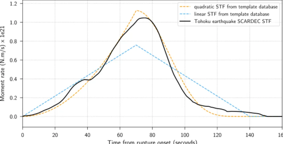
Figure 5. SCARDEC solution for the moment-rate STF of the M9.1 Tohoku earthquake (solid line), along with the closest
templates (dashed lines). STF templates grow either linearly (blue line) or quadratically (orange line) with time. STFs are normalized to 1 N.m in the template database but are here scaled to the event final moment for plotting purposes. STF = source time functions.
factor𝛼 is the least-squares estimate of the scaling factor between t and s, averaged over the sensors and components: 𝛼(t) = Ni ∑ i Nj ∑ j wij ∑N ntij(nΔt) sij(t − nΔt) ∑N ntij(nΔt)2 , (5)
with wij(t) the normalized weight corresponding to the SNR at the given station and component. The estimated earthquake moment is𝛼 times the template moment.
Templates are correlated fully or by parts, such that we monitor the growth of the rupture as soon as it begins. We point out that in comparison to conventional EEWS which estimate the final magnitude of an earthquake, our proposed system estimates the instantaneous magnitude, that is, the seismic moment released up to the time the estimate is made. In principle, at stations that are located beyond the P wave front at the earthquake end-time, rupture arrest can be diagnosed, and the final magnitude estimated.
4.3. Rupture Scenarios
To demonstrate the potential of a gravity-based EEWS, we focus on large offshore subduction earthquakes. We thus consider in this subsection rupture scenarios of the 2011 M9.1 Tohoku-oki earthquake and its M7.3 foreshock, as it would have been recorded by networks of gravity strain sensors. Two different networks of three gravity strainmeters are considered, one close to the ruptured areas (∼250 km from the epicenter) and the other at regional distances (∼1,100 km from the epicenter).
Gravity strain data are obtained through the sum of the analytical perturbations and the simulated instru-mental noises for two components of the gravity strain tensor (hEZand hNZ), as already performed in section 3. We choose here to consider the intermediate detector sensitivity model 1, with a gravity-strain sensitivity of 10−15Hz−1∕2at 0.1 Hz.
We use the Global Centroid Moment Tensor (Ekström et al., 2012) parameters for the epicenter coordinates (37.52∘ N, 143.05∘ E for the Tohoku event and 38.56∘ N, 142.78∘ E for its foreshock) and fault geometries (strike/dip/rake = 203∘/10∘/88∘ for the Tohoku event and 189∘/12∘/78∘ for its foreshock) and the STFs from the SCARDEC catalog (Vallée & Douet, 2016).
In order to build a template database, gravity strain Green’s functions are computed analytically for three different dip-slip fault mechanisms, which approximate the subduction context near the Japan Trench (strike = 180∘, 190∘, or 200∘, dip = 10∘, and rake = 90∘, depth 20 km). Two types of STF onset (linear and quadratic) and source half-durations ranging from 2 to 90 s are considered. It should be noted that the actual source solutions for the Tohoku event and its foreshock are not in the present template database. Examples from the STF database, along with SCARDEC solution, for the Tohoku earthquake are plotted in Figure 5. Additional
Figure 6. (New version) Offline real-time detection, source location, and magnitude estimation of the M9.1 Tohoku earthquake, 15 s after onset time. (left)
Gravity strainhEZandhNZrecordings (black lines), along with the best-fitting gravity strain template (red lines). (right) The red and green stars represent the earthquake epicenter location and its estimated location, Fifteen seconds after onset time, P (blue) and S wavefronts (red) have not yet reached the coasts, while a M7.4 earthquake is detected with a high LR (>55), close to the actual M7.7 magnitude. LR = likelihood ratio.
priors based on the geometry of major active faults in the area and a catalog of moment rate functions from past earthquakes could complement the template database in the future.
As an example, the gravity strain recordings 15 s after the Tohoku earthquake onset time, along with the corresponding optimal template, are shown for one rupture scenario in Figure 6. The earthquake would have been detected with a high LR (>50) and accurate estimates for the epicenter location, onset time, and released magnitude, 5 s before the P waves even hit the Japanese coastlines. The optimal template corresponds to a rupture still ongoing, while the lower bound magnitude estimate of the rupture (>M7.4) is high enough to issue a regional warning.
Figure 7. (New version) Offline real-time magnitude estimation of the M9.1 Tohoku earthquake, 100 s after onset time. (left) Gravity strainhEZandhNZrecordings (black lines), along with the best-fitting gravity strain template (red lines). (right) The epicenter location is supposed to be known. One hundred seconds after onset time, a>M9 earthquake is detected. LR = likelihood ratio.
Figure 8. (New version) Rupture scenarios of the M9.1 Tohoku earthquake (top) and its M7.3 foreshock (bottom). The
black lines represent the released magnitude (STF from the SCARDEC database), while the thick red lines represent the estimated magnitudes averaged over 100 iterations (bounded with the±1 standard deviation curves), inferred with model-1 sensors. The yellow panels indicate estimations provided by the network deployed close to the ruptured areas, and the blue panel estimations from the network at regional distance. Estimations are provided up to the seismic waves arrival at the network. The thick blue line represents the EEW magnitudes issued in real time during the M9.1 Tohoku earthquake by the Japan Meteorological Agency (JMA) (Hoshiba & Ozaki, 2014). EEW = earthquake early warning.
The seismic P wavefront reaches sensors considered in Figure 6 before the Tohoku earthquake end-time, such that an estimate of the earthquake final magnitude cannot be made based on these sensors. A network of gravity strainmeters located further away from the rupture area (beyond ∼1,000 km) could monitor the whole rupture. This is the case for the second network we considered. See for instance the gravity strain recordings and corresponding optimal templates 100 s after onset time in Figure 7.
A hundred different rupture scenarios for the M9.1 Tohoku earthquake and its M7.3 foreshock have been sim-ulated, with a different random realization of instrument noise computed for each scenario. The earthquake magnitudes are estimated in real time by the two networks of model-1 sensors; the corresponding results are displayed in Figure 8. The input seismic moment functions from the SCARDEC database are accurately retrieved.
Real-time magnitude estimates inferred by networks of model-1 to model-4 sensors and their corresponding LR are displayed in Figures S1 and S2, for the M9.1 Tohoku and M7.3 foreshock earthquakes. These results confirm the sensitivity of 10−15Hz−1∕2around 0.1 Hz (models 1, 2, and 4) is required to record high-LR signals
and provide precise magnitude estimations in real time. Recordings from model-1 and model-3 sensors 25 s after the M7.3 foreshock onset time are displayed in Figures S3 and S4 and further illustrate this requirement. To appreciate the magnitude uncertainties, we compute the standard deviation of the 100 estimated mag-nitudes from the random realizations. Based on the gravity strain data recorded by the local network, the LR exceeds 50 only 15 s after the Tohoku onset time, with a corresponding M7.54 ± 0.13 magnitude estimate (the actual released moment is M7.7). For the foreshock, LR exceeds 50 only 18 s after the onset time, with a corre-sponding M7.17 ± 0.13 magnitude estimate (actual released moment M7.31). In both cases, within 10 s of the rupture onset (at least 10 s before P waves arrived to the coast), it could have been determined that the earth-quake magnitude was likely to exceed M7. According to the SCARDEC STF, the Tohoku event released moment exceeded the M9 magnitude 83 s after its onset time. Our magnitude estimate based on gravity-strain data recorded by the regional network is, in this idealized exercise, in perfect agreement, as it reaches at that time M9.02 ± 0.03.
Estimates of seismic moment M0based on early P and S wave signals are usually highly uncertain and underes-timated (see for instance JMA warnings issued from seismic data in Figure 8). Robust estimates of M0for large earthquakes based on W-phases (Kanamori & Rivera, 2008) can be obtained after at least 20 min (Duputel et al., 2011). Seismogeodetic methods based on high-rate GPS data can, in principle, provide rapid source parameter estimates within a few tens of seconds of the earthquake initiation (Crowell et al., 2016; Ruhl et al., 2017). A robust estimate of M0derived from gravity signals might be obtained earlier and fully stable at the
end of the rupture, which could significantly enhance tsunami warning systems in the near-source region.
5. Conclusion
We have established key quantitative results regarding the capabilities that future gravity strainmeters could achieve for earthquake source characterization, based on earthquake-induced prompt gravity signals before direct seismic wave arrivals. We computed earthquake-induced prompt gravity strain signals with an analytical model in a homogeneous half-space and tested various gravity strainmeters sensitivity models. Considering the planned sensitivities of about 10−15Hz−1∕2at 0.1 Hz for the subhertz gravity strainmeters
under development for GW detection, we have demonstrated that prompt perturbations induced by earth-quakes larger than M7 can be observed with a single gravity detector at distances shorter than 1,000 km from the epicenter within the travel time of P waves (SNR> 10) and up to 120 km within 10 s of the earthquake onset time (SNR> 5).
Since gravity field fluctuations propagate essentially instantaneously in comparison with seismic waves, a very promising application of this study is the improvement of the performance of EEWS. We demonstrate that a potential benefit of a gravity-based EEWS compared to seismic-based EEWS is earlier warning for large offshore subduction earthquakes. Moreover, one of the current issues in EEWS is the estimation of the magni-tude of the event, especially for mega earthquakes. Our simulations illustrate how gravity strainmeters could accelerate the estimation of the magnitude of mega earthquakes, by providing robust magnitude estimates within the duration of the fault rupture. We therefore propose that gravity strain data have the potential to complement other geophysical data in the future, to enhance tsunami warning systems.
While the foregoing discussion presents key elements of a gravity-based EEWS, a thorough assessment of the feasibility of this concept requires further developments: gravity signal predictions in more realistic earth-quake scenarios that incorporate the effects of finite rupture size, Earth heterogeneities, attenuation and scattering, the analysis of the inverse problem of location and magnitude estimation to determine the optimal sensor network geometry, the assessment of the impact of nonstationary noise, and a cost-benefit anal-ysis of its integration with existing EEWS. The most difficult challenge will be the development of gravity gradiometers with strain sensitivity of about 10−15Hz−1∕2at 0.1 Hz.
References
Abbott, B., Abbott, R., Adhikari, R., Ajith, P., Allen, B., Allen, G., et al. (2009). LIGO: The laser interferometer gravitational-wave observatory.
Reports on Progress in Physics, 72(7), 76901.
Accadia, T., Acernese, F., Antonucci, F., Astone, P., Ballardin, G., Barone, F., et al. (2011). Status of the Virgo project. Classical and Quantum
Gravity, 28(11), 114002.
Allen, R. (2013). Seismic hazards: Seconds count. Nature, 502(7469), 29–31.
Allen, R. M., Gasparini, P., Kamigaichi, O., & Bose, M. (2009). The status of earthquake early warning around the world: An introductory overview. Seismological Research Letters, 80(5), 682–693.
Ando, M., Ishidoshiro, K., Yamamoto, K., Yagi, K., Kokuyama, W., Tsubono, K., & Takamori, A. (2010). Torsion-bar antenna for low-frequency gravitational-wave observations. Physical review letters, 105(16), 161101.
Beker, M., Cella, G., DeSalvo, R., Doets, M., Grote, H., Harms, J., et al. (2011). Improving the sensitivity of future GW observatories in the 1–10 Hz band: Newtonian and seismic noise. General Relativity and Gravitation, 43(2), 623–656.
Bose, S., Dayanga, T., Ghosh, S., & Talukder, D. (2011). A blind hierarchical coherent search for gravitational-wave signals from coalescing compact binaries in a network of interferometric detectors. Classical and Quantum Gravity, 28(13), 134009.
Cella, G. (2000). Off-line subtraction of seismic Newtonian noise. In R. Cianci, et al. (Eds.), Recent developments in general relativity. Genoa: Springer, pp. 495–503.
Cheinet, P., Canuel, B., Dos Santos, F. P., Gauguet, A., Yver-Leduc, F., & Landragin, A. (2008). Measurement of the sensitivity function in a time-domain atomic interferometer. IEEE Transactions on Instrumentation and Measurement, 57(6), 1141–1148.
Colombelli, S., Zollo, A., Festa, G., & Picozzi, M. (2014). Evidence for a difference in rupture initiation between small and large earthquakes.
Nature Communications, 5, 3958.
Crowell, B. W., Schmidt, D. A., Bodin, P., Vidale, J. E., Gomberg, J., Renate Hartog, J., et al. (2016). Demonstration of the Cascadia G-FAST geodetic earthquake early warning system for the Nisqually, Washington, earthquake. Seismological Research Letters, 87(4), 930–943. Driggers, J. C., Harms, J., & Adhikari, R. X. (2012). Subtraction of Newtonian noise using optimized sensor arrays. Physical Review D, 86(10),
102001.
Acknowledgments
We acknowledge the financial support from the UnivEarthS Labex program at Sorbonne Paris Cité (ANR-10-LABX-0023 and ANR-11-IDEX-0005-02) and the financial support of the Agence Nationale de la Recherche through the grant ANR-14-CE03-0014-01. J.-P. M. acknowledges the financial support of I.U.F. (Institut universitaire de France). J. P. A. acknowledges funding by the French government through the "Investissements d’Avenir UCAJEDI" project managed by the Agence Nationale de la Recherche (grant ANR-15-IDEX-01). We thank Tomofumi Shimoda for stimulating discussions. Numerical computations were partly performed on the S-CAPAD platform, IPGP, France. Python routines used to compute the expected gravity strain signal (Harms, 2016) and noise are available at the GitHub repository https://github.com/kjuhel/gravity-eew.
Duputel, Z., Rivera, L., Kanamori, H., Hayes, G. P., Hirshorn, B., & Weinstein, S. (2011). Real-time W phase inversion during the 2011 off the Pacific coast of Tohoku Earthquake. Earth, Planets and Space, 63(7), 535–539.
Dziewonski, A. M., & Anderson, D. L. (1981). Preliminary reference Earth model. Physics of the Earth and Planetary Interiors, 25(4), 297–356. Ekström, G., Nettles, M., & Dziewo ´nski, A. (2012). The global CMT project 2004–2010: Centroid-moment tensors for 13,017 earthquakes.
Physics of the Earth and Planetary Interiors, 200, 1–9.
Fiorucci, D., Harms, J., Barsuglia, M., Fiori, I., & Paoletti, F. (2018). Impact of infrasound atmospheric noise on gravity detectors used for astrophysical and geophysical applications. Physical Review D, 97, 62003.
Frank, W. B., Shapiro, N. M., Husker, A. L., Kostoglodov, V., Romanenko, A., & Campillo, M. (2014). Using systematically characterized low-frequency earthquakes as a fault probe in Guerrero, Mexico. Journal of Geophysical Research: Solid Earth, 119, 7686–7700. https://doi.org/10.1002/2014JB011457
Geiger, R. (2017). Future gravitational wave detectors based on atom interferometry. In G. Augar & E. Plagnol (Eds.), An overview of
gravitational waves: Theory, sources and detection (pp. 285–313). Paris, France: World Scientific.
Gibbons, S. J., & Ringdal, F. (2006). The detection of low magnitude seismic events using array-based waveform correlation. Geophysical
Journal International, 165(1), 149–166.
Griggs, C., Moody, M., Norton, R., Paik, H., & Venkateswara, K. (2017). Sensitive superconducting gravity gradiometer constructed with levitated test masses. Physical Review Applied, 8(6), 64024.
Harms, J. (2015). Terrestrial gravity fluctuations. Living Reviews in Relativity, 18(1), 3.
Harms, J. (2016). Transient gravity perturbations from a double-couple in a homogeneous half-space. Geophysical Journal International,
205(2), 1153–1164. https://doi.org/10.1093/gji/ggw076
Harms, J., Ampuero, J. P., Barsuglia, M., Chassande-Mottin, E., Montagner, J. P., Somala, S., & Whiting, B. (2015). Transient gravity perturbations induced by earthquake rupture. Geophysical Journal International, 201(3), 1416–1425.
Harms, J., DeSalvo, R., Dorsher, S., & Mandic, V. (2009). Gravity-gradient subtraction in 3rd generation underground gravitational-wave detectors in homogeneous media. arXiv preprint arXiv:0910.2774.
Harms, J., & Paik, H. J. (2015). Newtonian-noise cancellation in full-tensor gravitational-wave detectors. Physical Review D, 92(2), 22001. Harms, J., Slagmolen, B. J., Adhikari, R. X., Miller, M. C., Evans, M., Chen, Y., & Ando, M. (2013). Low-frequency terrestrial gravitational-wave
detectors. Physical Review D, 88(12), 122003.
Heaton, T. H. (1985). A model for a seismic computerized alert network. Science, 228, 987–991.
Heaton, T. H. (2017). Correspondence: Response of a gravimeter to an instantaneous step in gravity. Nature Communications, 8(1), 966. Hogan, J. M., Johnson, D. M., Dickerson, S., Kovachy, T., Sugarbaker, A., Chiow, S. W., et al. (2011). An atomic gravitational wave
interferometric sensor in low earth orbit (AGIS-LEO). General Relativity and Gravitation, 43(7), 1953–2009.
Hohensee, M., Lan, S. Y., Houtz, R., Chan, C., Estey, B., Kim, G., & Müller, H. (2011). Sources and technology for an atomic gravitational wave interferometric sensor. General Relativity and Gravitation, 43(7), 1905–1930.
Hoshiba, M., & Ozaki, T. (2014). Earthquake early warning and tsunami warning of the Japan Meteorological Agency, and their performance in the 2011 off the pacific coast of Tohoku earthquake (Mw 9.0), Early warning for geological disasters. Berlin, Heidelberg: Springer, pp. 1–28.
Houston, H. (2001). Influence of depth, focal mechanism, and tectonic setting on the shape and duration of earthquake source time functions. Journal of Geophysical Research, 106(B6), 11137–11150.
Jaranowski, P., & Królak, A. (2012). Gravitational-wave data analysis. Formalism and sample applications: The Gaussian case. Living Reviews in
Relativity, 15(1), 4.
Juhel, K., Montagner, J., Vallée, M., Ampuero, J., Barsuglia, M., Bernard, P., & Whiting, B. (2018). Normal mode simulation of prompt elastogravity signals induced by an earthquake rupture. Geophysical Journal International, 216, 935–947.
Kanamori, H., & Rivera, L. (2008). Source inversion of W phase: Speeding up seismic tsunami warning. Geophysical Journal International,
175(1), 222–238.
Madariaga, R. (1976). Dynamics of an expanding circular fault. Bulletin of the Seismological Society of America, 66(3), 639–666.
McManus, D., Forsyth, P., Yap, M., Ward, R., Shaddock, D., McClelland, D., & Slagmolen, B. (2017). Mechanical characterisation of the TorPeDO: A low frequency gravitational force sensor. Classical and Quantum Gravity, 34(13), 135002.
Meier, M. A., Ampuero, J., & Heaton, T. H. (2017). The hidden simplicity of subduction megathrust earthquakes. Science, 357(6357), 1277–1281.
Meier, M. A., Heaton, T., & Clinton, J. (2016). Evidence for universal earthquake rupture initiation behavior. Geophysical Research Letters, 43, 7991–7996. https://doi.org/10.1002/2016GL070081
Montagner, J. P., Juhel, K., Barsuglia, M., Ampuero, J. P., Chassande-Mottin, E., Harms, J., & Lognonné, P. (2016). Prompt gravity signal induced by the 2011 Tohoku-Oki earthquake. Nature Communications, 7, 13349. https://doi.org/10.1038/ncomms13349
Moody, M. V., Paik, H. J., & Canavan, E. R. (2002). Three-axis superconducting gravity gradiometer for sensitive gravity experiments. Review
of Scientific Instruments, 73(11), 3957–3974.
Pai, A., Dhurandhar, S., & Bose, S. (2001). Data-analysis strategy for detecting gravitational-wave signals from inspiraling compact binaries with a network of laser-interferometric detectors. Physical Review D, 64(4), 42004.
Paik, H. J., Griggs, C. E., Moody, M. V., Venkateswara, K., Lee, H. M., Nielsen, A. B., & Harms, J. (2016). Low-frequency terrestrial tensor gravitational-wave detector. Classical and Quantum Gravity, 33(7), 75003.
Romanowicz, B. (1992). Strike-slip earthquakes on quasi-vertical transcurrent faults: Inferences for general scaling relations. Geophysical
Research Letters, 19(5), 481–484.
Ruhl, C., Melgar, D., Grapenthin, R., & Allen, R. (2017). The value of real-time GNSS to earthquake early warning. Geophysical Research Letters,
44, 8311–8319. https://doi.org/10.1002/2017GL074502
Rundle, J. B. (1989). Derivation of the complete Gutenberg-Richter magnitude-frequency relation using the principle of scale invariance.
Journal of Geophysical Research, 94(B9), 12337–12342.
Scholz, C. H. (1982). Scaling laws for large earthquakes: Consequences for physical models. Bulletin of the Seismological Society of America,
72(1), 1–14.
Shelly, D. R., Beroza, G. C., & Ide, S. (2007). Non-volcanic tremor and low-frequency earthquake swarms. Nature, 446(7133), 305–307. Shimoda, T., Aritomi, N., Shoda, A., Michimura, Y., & Ando, M. (2018). Seismic cross-coupling noise in torsion pendulums. Physical Review D,
97(10), 104003.
background using a pair of torsion-bar antennas. Physical Review D, 89(2), 27101.
Vallée, M., Ampuero, J. P., Juhel, K., Bernard, P., Montagner, J. P., & Barsuglia, M. (2017). Observations and modeling of the elastogravity signals preceding direct seismic waves. Science, 358(6367), 1164–1168.
Vallée, M., & Douet, V. (2016). A new database of source time functions (STFs) extracted from the SCARDEC method. Physics of the Earth and
Planetary Interiors, 257, 149–157.
Winterflood, J. (2001). High performance vibration isolation for gravitational wave detection (PhD Thesis), University of Western Australia Perth.