HAL Id: hal-01705829
https://hal.archives-ouvertes.fr/hal-01705829
Submitted on 9 Feb 2018
HAL is a multi-disciplinary open access
archive for the deposit and dissemination of
sci-entific research documents, whether they are
pub-lished or not. The documents may come from
teaching and research institutions in France or
abroad, or from public or private research centers.
L’archive ouverte pluridisciplinaire HAL, est
destinée au dépôt et à la diffusion de documents
scientifiques de niveau recherche, publiés ou non,
émanant des établissements d’enseignement et de
recherche français ou étrangers, des laboratoires
publics ou privés.
Heuristic approach for forecast scheduling
Hind Zaaraoui, Zwi Altman, Sana Jemaa, Eitan Altman, Tania Jimenez
To cite this version:
Hind Zaaraoui, Zwi Altman, Sana Jemaa, Eitan Altman, Tania Jimenez. Heuristic approach for
forecast scheduling. IWSON 2018 - 7th International Workshop on Self-Organizing Networks, Apr
2018, Barcelona, Spain. pp.1-6. �hal-01705829�
Heuristic approach for forecast scheduling
Hind Zaaraoui∗, Zwi Altman∗, Sana Ben Jemaa∗, Eitan Altman† and Tania Jimenez ‡
∗Orange Labs
38/40 rue du G´en´eral Leclerc,92794 Issy-les-Moulineaux Email:{hind.zaaraoui,zwi.altman,sana.benjemaa}@orange.com
†INRIA Sophia Antipolis and LINCS, France
Email:[email protected]
‡Avignon University
Email:[email protected]
Abstract—Forecast Scheduling (FS) is a scheduling con-cept that utilizes rate prediction along the users’ trajectories in order to optimize the scheduler allocation. The rate prediction is based on Signal to Interference plus Noise Ratio (SINR) or rate maps provided by a Radio Envi-ronment Map (REM). The FS has been formulated as a convex optimization problem namely the maximization of an α−fair utility function of the cumulated rates of the users along their trajectories [1]. This paper proposes a fast heuristic for the FS problem based on two FS users’ scheduling. Furthermore, it is shown that in the case of two users, the FS problem can be solved analytically, making the heuristic computationally very efficient. Numerical results illustrate the throughput gain brought about by the scheduling solution.a
Index Terms—Forecast scheduler, alpha-fair, high mobil-ity, Radio Environment Maps, geo-localized measurements
I. INTRODUCTION
The concept of FS has been introduced in [1], where it is shown that the knowledge of the present and future rates along the users’ trajectories can be exploited by the scheduler in order to significantly improve the average user throughput. The throughput gain is achieved by exploiting long term time and spatial diversity along the users’ trajectory. The FS allocation is posed as a convex optimization problem that can be solved using fast convex optimziation solvers. The randomness of the traffic, i.e. arrival and departure of communications on the one hand and randomenss in the user trajectories on the other hand can be incorporated into the FS solution [2].
The SINR or rate along the mobile users’ trajectories can be provided using a REM. The generation of REMs from Geo-Localized Measurements (GLM) has been the topic of recent research activity in both industry and
aThis work has been partially carried out in the framework of
IDEFIX project, funded by the ANR under the contract number ANR-13-INFR-0006.
academia and is decribed in more details in Section II. While abundant work on REM construction has been published, little work is available on how to exploit GLM and REMs to better manage the network.
The reasons for the growing interest in exploiting GLM are the following: First, it allows network operators to better assess the actual Quality of Service (QoS) of mobile users at any location; Second, it provides significant levers to optimize the network performance; and third, it allows personalized, user centric type of op-timization. GLM can feed new Radio Resource Manage-ment (RRM) algorithms, and in general, a manageManage-ment entity to (self-) configure, optimize and troubleshoot the network. The use of GLM corresponds to a general trend in 5G networks, namely the exploitation of data from different sources in order to improve the network operation.
The purpose of this paper is to introduce a fast heuristic for the problem of calculating the FS allocation. Such a heuristic can simplify the implementation of the FS in real equipment. The contributions of this paper are the following:
• Provides an analytical solution for the FS allocation problem for the case of two mobile users;
• Develops a computationally fast FS allocation heuristic based on the solution for two mobile users. The paper is organized as follows: Section II provides an overview of REMs and illustrates how the FS can exploit the REM to achieve throughput gain. Section III recalls the basic FS formulation and provides the main results for a closed form allocation rule for the case of two users. Section IV presents a two users based FS heuristic. Numerical results are described in Section V followed by concluding remarks in Section VI.
II. RADIOENVIRONMENTMAPS
With the availability of Global Positioning System (GPS) information in most mobile terminals, it has
become possible to retrieve radio measurements together with their corresponding location. GLMs can be re-ported to the network using User Equipments (UEs) with chipsets that implement the Minimization of Drive Testing (MDT) feature standardized by the 3rd Genera-tion Partnership Project (3GPP) [3]. GLM comprises a rich source of information that allows network operators to optimize the network with finer granularity than the classical cell level, and to go one step further towards personalized optimization of the end-user experience.
As the measurements are performed by UEs, the operator does not have the control on the positions where these measurements are performed. Hence the first chal-lenge has been to complement the information provided by GLM namely predicting the considered quantity in the entire area of interest and to build the complete REM.
The concept of REM was first introduced in cognitive radio and TV whitespace database systems [4], [5]. In mobile networks, the main research has focused on building reliable maps that could be trusted by radio engineers and that could be integrated in automated optimization processes and tools.
Several works ([6], [7], [8]) have considered the geostatistical interpolation technique known as Kriging [9] to build REMs. This technique exploits the spatial correlation of the signal propagation to provide higher prediction accuracy than classical propagation models. The accuracy of the prediction can be enhanced by increasing the density of the measurement samples. However, the computational complexity of the algorithm increases rapidly with the number of measurement points n, namely as O(n3). The reduction of the computa-tional complexity has been among the main research challenges. The Fixed Rank Kriging (FRK) [10] solu-tion brings the computasolu-tional complexity of the REM construction to a linear level with respect to n, while maintaining high quality. The latter can be measured in terms of the root-mean square error (RMSE) of the interpolated GLM with respect to a reference test set of GLM for example. The coverage map is obtained using a ray tracing propagation model.
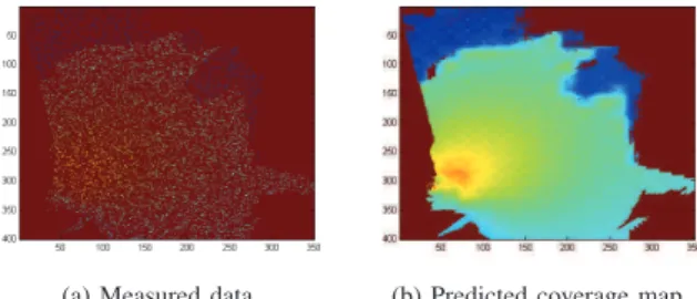
Figure 1(a) shows GLM of the received signal strength over 10 percent of the meshes in a cell area, and the predicted coverage area obtained using the FRK algorithm in Figure 1(b). In this example, the FRK is able to build the entire map with a root-mean square error not exceeding 3 dB.
Once the received signal strength coverage map is built with a satisfactory accuracy, it can serve as input to construct other radio measurement maps such as the SINR map. Figure 2(a) illustrates an SINR map with two trajectories drawn in blue and black. In Figure 2(b)
(a) Measured data. (b) Predicted coverage map.
Fig. 1. Coverage map prediction using FRK.
one can see the reachable bitrates that two vehicles will encounter while moving along the two trajectories using the Shannon formula. The significant spatial diversity in SINR and in the corresponding rate along the trajectories motivates the development of computationally efficient FSs.
(a) SINR map. (b) Theoretical bitrates.
Fig. 2. From SINR map to reachable bitrates.
III. FORECAST SCHEDULING MODEL AND ANALYTICAL RESULTS
In this Section we first briefly recall the basic formu-lation of the FS as presented in [1]. Then, using Karush-Kuhn-Tucker (KKT) conditions, we provide the main results for the closed form solution for n= 2 users. Due to space limitation, the complete formulation is given in a supplementary document [11].
A. Basic formulation
Consider a macro-cell (Base Station (BS)) surrounded by interfering BSs. We suppose that the SINR of the users in mobility at any location is provided to the BS by a REM. Consider n full buffer users moving at a constant speed during a time interval T - the scheduling period, over which n is considered constant. Suppose that time is in a discrete space: t∈ {1, 2, .., T } = [|1, T |] and let i denote the user number, i∈ {1, 2, .., n} = [|1, n|]. We suppose that during the scheduling duration there are no arrivals or departures of users (it is noted that this assumption can be relaxed [2]).
A scheduling period T (typically of the order of seconds) is divided into scheduling time slots e.g. of 1ms, during which the bandwidth is shared among the scheduled users. In practice, the time resolution of the FS is longer than the system time slot (e.g. of 1ms), and is referred to hereafter as time slot (see Section V). Let ai(t) denote the bandwidth proportion allocated to the user i at time t, ai(t) ∈ [0, 1] according to the scheduling strategy, where∀t, Pni=1ai(t) = 1, and W is the total bandwidth. Using the Shannon equation, the throughput as a function φ of the SINR of user i reads
ai(t)φ(SIN Ri(t)) = ai(t)W log2(1 + SIN Ri(t)). (1)
Denote by Sitthe predicted SINR (i.e. the one provided by the REM). The FS allocation policy is defined by the following optimization problem, with α6= 1:
maximize: f (a) = n X i=1 (PTt=1ai(t)φ(S t i)) 1−α 1 − α (2) subject to: ∀i, ∀t, ai(t) ≥ 0 ∀t, n X i=1 ai(t) = 1.
α is a positive fixed parameter of the optimization problem. For α→ 1, the optimization problem with the same constraints reads:
maximize: f (a) = n X i=1 log( T X t=1 ai(t)φ(S t i)). (3)
Both equations (2) and (3) have concave functions f for α≥ 0, and can be solved using convex optimization (e.g. CVX solver [12], see more details in Section V). The size of the optimization problem is defined by the number of unknown variables, namely n× T (with T being the number of time slots).
The interpretation of (2) and (3) is the following: resources are shared fairly among the users according to the data-rate variation along their trajectories. For example, if a user has a large enough coverage hole in his future trajectory, the FS may allocate to this user as much data as possible before reaching the coverage hole so as to remain fair with respect to the other users.
B. KKT conditions
We first derive the KKT conditions for the problem (2). The optimization problem (2) has a nonlinear objective function f with regular equality and inequality conditions i.e. differentiable constraint functions. If the objective and constraint functions (2) are continuously differen-tiable at any a = (a1(1), ...a1(T ), a2(1), ..., an(T )) ∈
RnT, then there exist multipliers λ
k,j and νj, where k∈ [|1, n|] and j ∈ [|1, T |], called KKT multipliers ([13], Chap.5) with the following Lagrangian function:
L(a, ν, λ) = f (a)+ T X j=1 νj( n X k=1 ak(j)−1)+X k,j λk,jak(j), (4) where λk,j≥ 0.
We define the Lagrange dual function as the maximum value of L over a. Let a∗ maximize the Lagrangian function (4) for the optimal multipliers λ∗k,j and νj∗, where k ∈ [|1, n|] and j ∈ [|1, T |], and therefore its gradient is null at this point:
∇L(a∗, ν∗, λ∗) = 0. (5) From (5) one obtains for all i∈ [|1, n|] and t ∈ [|1, T |] the corresponding KKT conditions:
φ(St i)( T X j=1 a∗i(j)φ(Sij))−α+ ν∗ t + λ∗i,t = 0, (6) a∗i(t) ≥ 0, (7) n X k=1 a∗k(t) = 1, (8) λ∗i,ta∗i(t) = 0 (9) λ∗i,t ≥ 0. (10) We note from (6) that for any time t, for all users i and w with w6= i φ(Sit)( T X j=1 a∗i(j)φ(Sij))−α+ λ∗i,t = φ(Swt)( T X j=1 a∗w(j)φ(Swj))−α+ λ∗w,t (11)
and also from (6), for all user i, we have for any time t and u: λ∗i,t+ ν∗ t φ(St i) = λ ∗ i,u+ νu∗ φ(Su i) (12) as ν∗
t does not depend on the users, and PT
j=1a∗i(j)φ(S j
i) does not depend on the time. Equality (11) gives explicitly the resource balancing among users at each time relatively to α in the sense of equalizing the two expressions for each user.
C. Analytical solution for n= 2 users
In the calculations that follow, we rewrite a = a∗, λ = λ∗ and ν = ν∗. We assume two users in the cell, i.e. n= 2 in problem (2).
KKT analysis shows that there exists at most one time slot K ∈ [1, T ] for which two users can be scheduled simultaneously [11]. For all other times in[1, T ] one user is scheduled at a time. We formulate hereafter the more frequent case where there is no K ∈ [1, T ] for which two users scheduled at the same time. The complete analysis is available in [11].
We suppose in this section that at time u= 1 user 1 is scheduled and therefore λ1,1 = 0. We need to verify this assumption, namely that user 1 is indeed selected at time u= 1 (see Theorem 2). For all time t, the sign of λ1,t− λ2,t determines the scheduling decision: if it is positive then user 2 is scheduled at time t (λ1,t ≥ λ2,t⇐⇒ a2(t) ≥ a1(t) by equations (9-10)). One of the lambdas must be null and the other one positive for the case of two users.
Using equation (12), as λ1,1= 0, we have: λ1,t− λ2,t= ν1ψ1t/1− ν1ψ t/1 2 − λ2,1ψ t/1 2 (13) where ψit/u= φ(Sti) φ(Su i). We have then: λ1,t− λ2,t= ν1(ψt/11 − ψ t/1 2 ) − λ2,1ψ t/1 2 (14) As λ2,1ψ2t/1 > 0 we divide equation (14) by λ2,1ψ2t/1 and hence the sign studied is the same as the sign of
ψt/1 2 −ψt/11
ψt/12
−λ2,1
ν1
− 1. Note that from (6), ν1is negative. If ψt/12 < ψ1t/1then λ1,t− λ2,t<0 hence user 1 will be scheduled at time t. We cannot say more using this method.
Theorem 1. If user 1 is supposed scheduled at time u= 1, then:
ψt/12 < ψ1t/1=⇒ user 1 is scheduled at time t. Denote by Au1 and Au2 the following sets:
Au1 = {t 6= u, ψ1t/u> ψ t/u 2 } ∪ {u} Au2 = {t 6= u, ψt/u1 < ψ2t/u} For u= 1 and using Theorem 1 i.e. if t ∈ Au
1 then we have that user 1 is surely scheduled at time t > 1 with the assumption that the user is scheduled at time1. We have the following result:
Theorem 2. User 1 is scheduled at time u if and only
if: (X Au 2 φ(S2j))α> max k∈Au 1 φ(Sk 2) φ(Sk 1) (X Au 1 φ(Sj1))α (15)
Equivalent scheduling rule can be written for user 2. The proof of the theorem is given in [11].
IV. HEURISTIC SOLUTION FORFORECAST
SCHEDULING
In this section, we propose a heuristic FS solution for an arbitrary number of users n which relies on FS with n= 2 users.
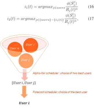
Consider an iterative algorithm for scheduling user(s) at time t with two main steps: (i) choose two users, i1 and i2with the highest α-fair utility given by equations (16) and (17) where Rj(t) is the mean past data rate (calculated over some time window) of the user j until time t; (ii) Select the best user (or both users) according to the FS rule for n = 2 for the time interval [|1, T |]. It is recalled that FS for n= 2 can be computed using closed form formula or using a fast convex optimization solver. The algorithm is depicted in Table I.
i1(t) = argmaxj∈users φ(S t j) Rj(t)α (16) i2(t) = argmaxj∈{users}−{i1(t)} φ(St j) Rj(t)α, (17)
Fig. 3. Scheduling using the best two α−fair heuristic.
The user selection algorithm in Table I is not as optimal as the direct FS technique since it considers only the future SINR trajectories of the two best α−fair users. Interestingly, this approach provides significant gains with respect to Round Robin (RR) scheduler. It is recalled that at high mobility, the Proportional Fair (PF) scheduling converges to RR due to the short coherence time of the channel.
It is noted that alternatively and with a higher com-plexity, Step 2 in Table I can be performed using the FS for the two users selected in step 1 using a convex optimization solver.
TABLE I
TWOBESTUSERSALGORITHM(TBUA) Algorithm of approximation with two best α-fair users
Step 1 -Select the two best users i1and i2
accord-ing to (16) and (17) at time t
Step 2 -Apply KKT resolution for the case of two
users for i1and i2. Verify if time K exists
(using (19) in [11]). If it exists, use allo-cation (16-18) in [11]. Otherwise use (15), and select the user to schedule at time t accordingly (using the condition in Theorem 1) .
Step 4 -Update the mean past data rate for all users
utilizing the received data rate at time t
Step 5 -if t+1 ≤ T proceed to time t+1, T being
the scheduling period
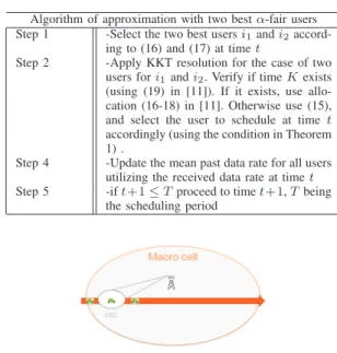
Fig. 4. A road crossing a cell and the coverage area of a VSC.
V. NUMERICAL RESULTS
This Section presents numerical results for the FS heuristic obtained using a Long Term Evolution (LTE) network simulator written in Matlab. We consider a scenario with 10 vehicular users moving with a constant speed of 50km/h along a road crossing the cell. Close to the cell edge, the road traverses a coverage area of a Virtual Small Cell (VSC). It is recalled that the VSC is a remotely created small cell using a Large Scale Antenna System (LSAS) [14] which is used to enhance the spatial SINR diversity along the trajectory (see Figure 4).
The spatial resolution of the REM is of 1m (which is feasible thanks to the interpolation of the GLM. The corresponding time interval at 50km/h is 70ms over which the SINR is considered constant. This time interval defines the time resolution of the FS during which a fixed allocation is applied, i.e. the same users are scheduled at time intervals defined by the technology (e.g.1ms for LTE). The SINR experienced by the users along the road is presented in Figure 5. The first (stronger) and second maxima correspond to the transmissions at the vicinity of the VSC and the macro BS respectively. Simulation parameters are depicted in Table II.
In the following, we compare the TBUA solution with the (standard) FS solution of problem 3. The FS solution is solved using CVX (details below). The TBUA is solved using the heuristic solution described in Section IV with the analytical FS of Section III-C.
0 50 100 150 200 250 300 0 50 100 150 200 250 Iteration (1 iteration = 70ms) SINR (linear)
Fig. 5. SINR for different users along the road.
TABLE II SIMULATION PARAMETERS
Network parameters
Number of macro-cell BSs 1
Number of interfering BSs 6
Macro-cell layout hexagonal omni sectors
Intersite distance 500 m
Bandwidth 20 MHz
Channel characteristics
Thermal noise −174 dBm/Hz
Macro Path loss (d in km) 128.1 + 37.6log10(d) dB
Mobility traffic characteristics
User speed 50 km/h
Number of users 10
File size σ full buffer (∞)
One iteration = Scheduling delay 70 ms
We assume that the interfering neighboring cells have 10 percent of load (details on the interference model can be found in [1]). The interference conditions when using the REM will differ from those used to create the REM. We denote this as interference errors in the sequel. To show the robustness of the FS with respect to interference errors, we consider two cases: (i) a REM constructed with fully (100 percent) loaded interfering cells, which is denoted hereafter as ”with interference errors” and (ii) a hypothetical REM that provides the exact SINR, namely 10 percent of loaded interfering cells, and is denoted as ”without interfering errors”.
Reference [1] explains that the scheduling decisions of the FS can be impacted to a certain extent by the interference errors, and the impact of these errors de-creases with the increase in the scheduling periodicity. Moreover, the impact of the interference errors on the Mean User Throughput (MUT) is negligible. This be-havior is explained by the high spatial dynamicity of SINR variations, the trends of which are well captured by the REM in spite of the interference errors. We consider the RR as a baseline for the different approaches. The rationale is that at high mobility considered here, the coherence time is too short to exploit fast fading in order to achieve opportunistic scheduling gain.
The objective functions of the optimization problems (2) and (3) are convex and can be solved using a convex
optimization solver. The CVX Matlab library has been used (see [12] and [15]). The CVX solver verifies the convexity of the problem and solves it using SDPT3 or SeDuMi. SDPT3 implements the infeasible path-following algorithms for solving conic programming problems whose constraint cone is a product of semi-definite cones. It uses a predictor-corrector primal-dual path-following method, with different types of search di-rection. SeDuMi is a linear/quadratic/semi-definite solver. The MUT time evolution for the 10 users and for the three different FS solutions with 2s periodicity: the (standard) FS with and without interference errors, the TBUA heuristic with interference errors, and for the baseline RR are presented in Figure 6. One can observe oscillations that are correlated with the SINR variations (see Figure 5). Most of the time, the TBUA varies between the FSs and the RR scheduling. The curves for the FSs and TBUA solutions are most of the time above those of the RR scheduling. As stated above, the impact of interference errors is negligible, which is an important characteristic of the FS based solutions.
0 50 100 150 200 250 300 2.5 3 3.5 4 4.5 5 5.5 6 6.5 7 7.5 Iteration (1 it. = 70 ms)
Normalized MUT (bits
/s
/Hz)
Forecast scheduling without interference error MUT in time Forecast scheduling with interference error MUT in time 2 best users algorithm MUT in time
RR MUT in time
Fig. 6. Time variation of users’ throughput for a scheduling period of T=2s, averaged over a sliding window of 15 iterations.
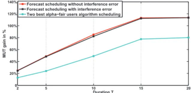
Figure 7 compares the MUT gain with respect to the baseline RR for the ten users, averaged along the full trajectory crossing the cell, for different FS scheduling periodicities. For 2s periodicity, the MUT gain for the TBUA and FS is of 15 and 30 percent respectively, and it grows monotonically to 80 and 117 percent respectively for 20s periodicity. One can observe a close to linear monotonic growth of MUT gain till 15s scheduling priod-icity, with non-significant improvement brought about the long term time-space diversity beyond this periodicity.
VI. CONCLUSION
The allocation of FS involves the solution of a convex optimization problem. The solution complexity scales up with the number of users and the scheduling duration. In view of reducing the computational complexity of the FS we have proposed a two step heuristic in which, for
2 5 10 15 20 0 20% 40% 60% 80% 100% 120% 140% Duration T MUT gain in %
Forecast scheduling without interference error Forecast scheduling with interference error Two best alpha!fair users algorithm scheduling
Fig. 7. FS MUT gain with and without interference errors, and TBUA wrt the RR scheduler as a function of the scheduling period (in sec).
each scheduling period, we select the two users with the highest α−fair utility and then we apply to them the FS. It has been shown that for n= 2, the FS allocation can be written in a closed form, making the heuristic even more computational efficient. Numerical simulations show that the throughput gain achieved by the FS heuristic remains significant, even for short scheduling periodicity.
REFERENCES
[1] H. Zaaraoui et al., “Forecast scheduling for mobile users,” in IEEE International Symposium on Personal, Indoor, and Mobile Radio Communications (PIMRC), 2016.
[2] ——, “Forecast scheduling and its extensions to account for random events,” in 21st Innovations in Clouds, Internet and Networks (ICIN 2018) Conference.
[3] W. Hapsari et al., “Minimization of drive tests solution in 3GPP,” IEEE Communications Magazine, vol. 50, no. 6, pp. 28–36, 2012. [4] B. A. Fette, Cognitive radio technology. Academic Press, 2009. [5] Y. Zhao et al., Network support–The radio environment map.
Elsevier.
[6] J. Ojaniemi et al., “Optimal field measurement design for radio environment mapping,” in IEEE 47th Annual Conference on Information Sciences and Systems (CISS), 2013, pp. 1–6. [7] A. Konak, “A kriging approach to predicting coverage in wireless
networks,” International Journal of Mobile Network Design and Innovation, vol. 3, no. 2, pp. 65–71, 2009.
[8] J. Riihijarvi et al., “Characterization and modelling of spectrum for dynamic spectrum access with spatial statistics and random fields,” in IEEE 19th International Symposium on Personal, Indoor and Mobile Radio Communications, 2008, pp. 1–6. [9] J. P. Chil`es and P. Delfiner, Geostatistics, Modeling Spatial
Uncertainty, 2nd ed. New-York: John Wiley & Sons, 2012. [10] N. Cressie et al., “Fixed rank kriging for very large spatial data
sets,” Journal of the Royal Statistical Society: Series B (Statistical Methodology), 2008.
[11] H. Zaraoui et al., “Analytical results for two users’
forecast scheduling,” November 2017. [Online]. Available: https://hal.inria.fr/hal-01633361
[12] I. CVX Research, “CVX: Matlab software for disciplined convex programming, version 2.0,” http://cvxr.com/cvx, Aug. 2012. [13] S. Boyd et al., Convex optimization. Cambridge university press,
2004.
[14] A. Tall et al., “Virtual sectorization: design and self-optimization,” in 5th International Workshop on Self-Organizing Networks (IW-SON 2015), Glasgow, Scotland, May 2015.
[15] V. Blondel et al., Recent advances in learning and control. Springer, 2008.