Bond slip model for the simulation of reinforced concrete structures

HAL Id: hal-01411079

https://hal.parisnanterre.fr//hal-01411079

Submitted on 16 Apr 2021

HAL is a multi-disciplinary open access

archive for the deposit and dissemination of sci-entific research documents, whether they are pub-lished or not. The documents may come from teaching and research institutions in France or abroad, or from public or private research centers.

L’archive ouverte pluridisciplinaire HAL, est destinée au dépôt et à la diffusion de documents scientifiques de niveau recherche, publiés ou non, émanant des établissements d’enseignement et de recherche français ou étrangers, des laboratoires publics ou privés.

Bond slip model for the simulation of reinforced

concrete structures

Anaelle Casanova, Ludovic Jason, Luc Davenne

To cite this version:

Anaelle Casanova, Ludovic Jason, Luc Davenne. Bond slip model for the simulation of reinforced concrete structures. Engineering Structures, Elsevier, 2012, 39, pp.66–78. �10.1016/j.engstruct.2012.02.007�. �hal-01411079�

1

Bond slip model for the simulation

of reinforced concrete structures

A. Casanova* , _{**, L. Jason*, L. Davenne***}

* CEA, DEN, DANS, DM2S, SEMT, LM2S, F-91191 Gif sur Yvette, France

** Laboratoire de Mécanique et Technologie (LMT), ENS Cachan, F-94235, Cachan, France *** IUT de Ville d’Avray, F-92410 Ville d’Avray, France

Abstract:

This paper presents a new finite element approach to model the steel-concrete bond effects. This model proposes to relate steel, represented by truss elements, with the surrounding concrete in the case where the two meshes are not necessary coincident. The theoretical formulation is described and the model is applied on a reinforced concrete tie. A characteristic stress distribution is observed, related to the transfer of bond forces from steel to concrete. The results of this simulation are compared with a computation in which a perfect relation between steel and concrete is supposed. It clearly shows how the introduction of the bond model can improve the description of the cracking process (finite number of cracks).

I

Introduction

Reinforced concrete structures may have to fulfill functions that go beyond their simple mechanical resistance. In some cases, information about the cracking behavior related to the quasi-brittle evolution of concrete can also become essential. For example, in the case of containment buildings for nuclear power plants, cracking has a direct impact on the transfer properties that govern the potential leakage rate (damage – permeability law (Picandet et al, 2001) among others). Predicting the mechanical behavior but also characterizing the crack evolution (opening and spacing) are thus key points in the evaluation of this type of reinforced concrete structures.

Cracking in reinforced concrete structures is generally influenced by the stress distribution along the interface between steel and concrete. For example, in the case of a reinforced tie, once the first crack appears in the weakest point of the structure, the concrete stress in the cracked zone drops to zero while the load is totally supported by the steel reinforcement. The stresses are then progressively transferred from steel to concrete (Figure 1). This transition zone has an impact on the crack properties and is directly influenced by the steel-concrete interface (Eurocode 2, 2007). Taking into account these effects seems thus essential to predict correctly the cracking of reinforced concrete structures.

2

c



Concrete Steel st c



s



Transition zone F F c



Concrete Steel st c



s



Transition zone F F

Figure 1 : Distribution of stresses in steel and concrete in a reinforced concrete tie after the first crack (



_cand



_sare the stresses in concrete and steel respectively, and



_cst is the concrete strength).

Different models exist to represent the steel-concrete bond behavior. For example, Ngo and Scordelis (1967) proposed a spring element, associated with a linear law, to relate concrete and steel nodes. To improve the description of the bond behavior, joint elements were developed. These zero thickness elements, introduced at the interface between steel and concrete, allow the use of a non linear law (Clément, 1987), (Daoud, 2003), (Lowes et al, 2004), (Dominguez et al, 2005), (Boulkertous 2009) and (Richard et al, 2010). Finally, special finite elements are proposed to enclose, in a same element, the material behavior (steel or/and concrete) and the bond effects (Monti et al 1997). Dominguez (2005) and Boulkertous, (2009), among others, developped embedded elements whose principle is to describe the steel-concrete bond behavior through an enrichment of the degrees of freedom (Figure 2). Even if these solutions give appropriate results, one of their main drawbacks, in the context of industrial applications, is the need to explicitly consider the interface between steel and concrete. It may impose meshing difficulties and heavy computational cost which are not compatible with large scale simulations. Concrete Steel Zero thickness k_n k_l Concrete Steel Zero thickness k_n k_l Concrete Steel Joint element Zero thickness Concrete Steel Joint element Zero thickness Embedded element Embedded element

Degrees of freedom of concrete Degrees of freedom of concrete

+ steel-concrete slip Degrees of freedom of concrete Degrees of freedom of concrete

+ steel-concrete slip

Figure 2 : Examples of bond elements (at the top left: spring element, at the top right: joint element, at the bottom: embedded element)

3

To overcome these difficulties, a perfect relation between steel and concrete is generally considered for structural applications and the reinforcement is modeled using truss elements. This hypothesis imposes the same strain in both materials. Although this approach simplifies the simulation, it is not fully representative of the experimental behavior (Figure 1).

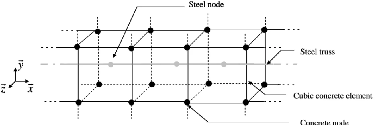
In this contribution, a model is proposed to combine the advantages of the two approaches. It will be able to represent the bond effects (the evolution of the slip between steel and concrete especially) and will be appropriate for structural applications (mesh and computational cost). The general configuration is to consider steel truss elements and concrete (1D, 2D or 3D elements) in the case where steel and concrete nodes are not necessary coincident (Figure 3).

Concrete node Steel node

Cubic concrete element Steel truss

x



y



z



Concrete node Steel node

Cubic concrete element Steel truss

x



y



z



x



y



z



Figure 3 : Description of the problem (steel and concrete nodes are not coincident)

The theoretical formulation of the model is presented in the first section. It is then validated in the second section on the case of a reinforced concrete tie. Finally, the influence of the bond effect is investigated by a comparison with a simulation using the hypothesis of a perfect relation.

II Description of the bond model

In reinforced concrete structures, the relation between steel and concrete is governed by a bond stress distributed along the interface. The evolution of this bond stress is generally studied in the form of a bond stress-relative displacement (slip between steel and concrete) curve (Figure 4). Therefore, the bond behavior can be represented by a bond stress-slip (



-

s

) law

f

_bdefined by:

)

(s

f

_b





₍₁₎

To take this effect into account, the principle of our approach is to introduce internal forces on both steel and concrete in the direction of the steel truss element.

4

Figure 4 : Shape of the bond stress-slip law (Eligehausen et al, 1983)

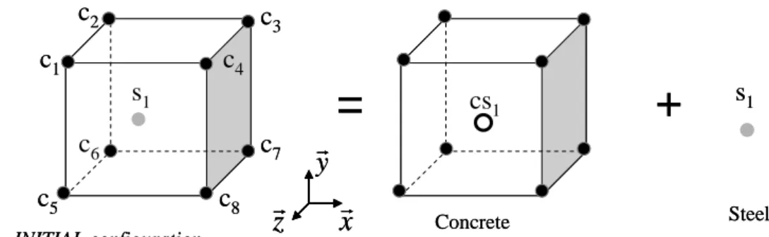
As concrete and steel nodes are not necessary coincident, each steel node is thus associated with the concrete element in witch it is included and with a tangential direction

t



.

In this contribution, equations will be developed in the particular case of a unique steel node inside a cubic concrete element as illustrated in Figure 5 (initial configuration). In order to simplify the equations,

t



coincides with the principal direction

x



.

The formulation of the model is divided into 4 steps:

- The evaluation of the steel-concrete slip with non coincident meshes - The calculation of the nodal bond forces in the steel element direction - The introduction of kinematic relations in the normal directions

- The implementation of the model within the small displacements theory

II.1 Evaluation of the relative displacement between steel and concrete

The steel-concrete slip is represented by the relative displacement in the x direction between the steel (

u

_s1 at node s1) and the concrete at the steel node (

u

cs1 at virtual point cs1) (Figure 5).

x cs x s u u s 1,  1, (2) with

u

_s1,x



u

 

_s1

x



and

u

_cs1,x



u

 

_cs1

x



.

As the meshes are not necessary coincident, the displacement in concrete at the steel node is obtained using the shape functions, following the equation:







8 1 , 1 1 1 , 1

(

,

,

)

i x ci cs cs cs i x cs

N

x

y

z

u

u

(3)

where

(

x

_cs1

,

y

_cs1

,

z

_cs1

)

are the coordinates of cs1 point.

N

i

(

x

cs1

,

y

cs1

,

z

cs1

)

represents the shape

function of the i-th concrete node evaluated at cs1 point and

u

ci,x its displacement in the

x



5

=

+

Concrete

x



y



z



INITIAL configuration Steel

s

₁

c

₁

c

₂

_c

3

c

₄

c

₅

c

₆

c

₈

c

₇ x c

u



_2,

u



_c3,x x c

u



_5, x c

u



_7, x c

u



_8,

x



y



z



cs

₁ x c

u



_4,

s

₁ x s

u



_1, x cs

u



_1, DEFORMED configuration x cs x s

u

u

s



_1,



_1, x c

u



_1,





8 .. 1 , , 1 1 1  i z y x Ni cs cs cs x c u_4, x c u_6, x c

u



_6, x c

u



_4, x c

u



_1, x s

u



_1,

=

+

Concrete

x



y



z



x



y



z



INITIAL configuration Steel

s

₁

c

₁

c

₂

_c

3

c

₄

c

₅

c

₆

c

₈

c

₇ x c

u



_2,

u



_c3,x x c

u



_5, x c

u



_7, x c

u



_8,

x



y



z



x



y



z



cs

₁ x c

u



_4,

s

₁ x s

u



_1, x cs

u



_1, DEFORMED configuration x cs x s

u

u

s



_1,



_1, x c

u



_1,





8 .. 1 , , 1 1 1  i z y x Ni cs cs cs x c u_4, x c u_6, x c

u



_6, x c

u



_4, x c

u



_1, x s

u



_1,

Figure 5 : Evaluation of the relative displacement between steel and concrete

II.2 Nodal forces in the tangential direction

From equations (1), (2) and (3), the bond stress is computed:



















 8 1 , 1 1 1 , 1

(

,

,

)

i x ci cs cs cs i x s b

u

N

x

y

z

u

f



(4)

The internal nodal force induced by concrete on steel,

F

cs1 s/ 1



, is calculated using the equation:

x

u

z

y

x

N

u

f

l

d

x

l

d

F

i x ci cs cs cs i x s b s s s cs































 8 1 , 1 1 1 , 1 1 / 1







*

(

,

,

)

with































 

0

)

,

,

(

1

0

)

,

,

(

1

8 1 , 1 1 1 , 1 8 1 , 1 1 1 , 1 i x ci cs cs cs i x s i x ci cs cs cs i x s

u

z

y

x

N

u

if

u

z

y

x

N

u

if





(5)

where

d

_s is the diameter of the steel bar and

l

is derived from the length of the steel elements connected to the node s1. For example, in Figure 6:

2

2

1 l

l

6

1

l

l

₂ 1

s

Steel mesh

2

2 1

l

l

l





1

l

l

₂ 1

s

Steel mesh 1

l

l

₂ 1

s

Steel mesh

2

2 1

l

l

l





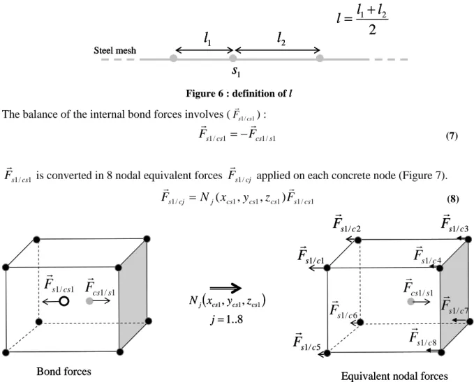
Figure 6 : definition of l

The balance of the internal bond forces involves (F_s1/cs1) :

1 / 1 1 / 1 cs cs s s

F

F









(7) 1 / 1 cs s

F



is converted in 8 nodal equivalent forces

F



_s1/cj applied on each concrete node (Figure 7).

1 / 1 1 1 1 / 1 cj j

(

cs

,

cs

,

cs

)

s cs s

N

x

y

z

F

F







(8) x c

u



_4, x c

u



_6, 1 / 1 cs s

F



1 / 1 s cs

F



u

c4,x



x c

u



_6,

Bond forces _{Equivalent nodal forces}

1 / 1 s cs

F



1 / 1 c s

F



2 / 1 c s

F



F



_{s1 c/ 3} 4 / 1 c s

F



5 / 1 c s

F



6 / 1 c s

F



F

s1 c/ 7



8 / 1 c s

F







8 .. 1 , , _{1 1} 1  j z y x N_{j cs cs cs} x c

u



_4, x c

u



_6, 1 / 1 cs s

F



1 / 1 s cs

F



u

c4,x



x c

u



_6,

Bond forces _{Equivalent nodal forces}

1 / 1 s cs

F



1 / 1 c s

F



2 / 1 c s

F



F



_{s1 c/ 3} 4 / 1 c s

F



5 / 1 c s

F



6 / 1 c s

F



F

s1 c/ 7



8 / 1 c s

F







8 .. 1 , , _{1 1} 1  j z y x N_{j cs cs cs}

Figure 7 : Balance of the internal bond forces

II.3 Kinematics relations in normal the normal directions

Equations (5) and (8) relate the degrees of freedom of concrete and steel in the tangent direction of the reinforcement. In the other directions, a perfect relation is supposed for the displacement. Two equations are thus added to close the system:

























  8 1 , 1 1 1 , 1 , 1 8 1 , 1 1 1 , 1 , 1

)

,

,

(

)

,

,

(

i z ci cs cs cs i z cs z s i y ci cs cs cs i y cs y s

u

z

y

x

N

u

u

u

z

y

x

N

u

u

(9)

II.4 Implementation of the bond element model

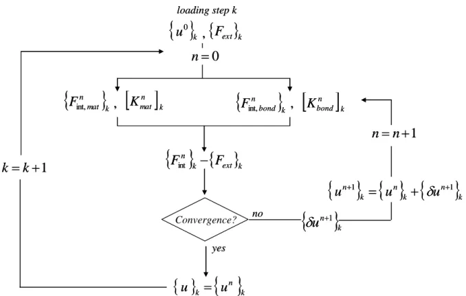
This bond model has been implemented in the finite element code Cast3M (Cast3M, 2010). For non linear problems (material and/or bond law), a Newton Raphson iterative method is used. In its

7

classical form, the nodal displacement

 

u

n1 at the n+1th iteration is calculated following equation (10).

 

 

 



n



mat ext n n mat

u

F

F

K



1





_{int, (10)} where

     

u

n1



u

n





u

n1 .

In this expression

 

F

_ext represents the external forces,



F

_int,n_mat



the usual internal forces induced by concrete and steel and

 

K

_matn the stiffness matrix at iteration n.

As describe in the previous sections, to take into account the bond effects, kinematics relations and bond forces are added. The kinematics equations (9) are introduced using the Lagrange’s multiplier method. Global internal bond forces



F

_int,n_bond



are calculated from equations (5) and (8) using the distribution of the nodal displacements at iteration n. Internal forces thus become:

  

 

n



bond n mat n

F

F

F

_int



_int,



_{int, (11)}

The global stiffness matrix

 

K

n is also updated:

    

n



bond n mat n

K

K

K





(12) where :





n u n bond n bond

u

F

K







int, (13)

The system finally becomes:

 

 

 

 

n ext n n

F

F

u

K



1





_{int (14)}

8

 

F

ext _k

 

u

k 0



n



_k mat

F

_int,





k n bond

F

_int,

 

k n

u

1



 

 

n _k k

u

u



     

k n k n k n

u

u

u

1







1 loading step k

 

k n mat

K

 

k n bond

K

,

,

Convergence? no yes

,

 

n _k

 

_{ext k}

F

F

_int



1



 n

n

1



 k

k

0



n

 

F

ext _k

 

u

k 0



n



_k mat

F

_int,





k n bond

F

_int,

 

k n

u

1



 

 

n _k k

u

u



     

k n k n k n

u

u

u

1







1 loading step k

 

k n mat

K

 

k n bond

K

,

,

Convergence? no yes

,

 

n _k

 

_{ext k}

F

F

_int



1



 n

n

1



 k

k

0



n

Figure 8 : Iterative diagram for the numerical resolution

III Validation and application of the bond model

In this part, the model is applied on a uniaxial problem. A reinforced concrete tie is studied in order to evaluate the influence of the bond effects on the mechanical behavior.

III.1 Presentation of the problem

A concrete cylinder reinforced with a longitudinal steel bar is considered. A displacement is imposed at the first end of the steel reinforcement while the other end is blocked (Figure 9). There are no boundary conditions on the concrete.

0

x

L

u



a

Cylinder of concrete Steel reinforcement

0

x

L

u



a

Cylinder of concrete Steel reinforcement

9

For the simulation, concrete and steel are meshed by truss elements. The total length L (equal to 3 meters) is divided into 100 identical trusses as illustrated in Figure 10.

steel concrete

u



L

0

L/100 Steel-concrete bond

a

steel concrete

u



L

0

L/100 Steel-concrete bond steel concrete

u



L

0

L/100 Steel-concrete bond

a

Figure 10 : Mesh of the tie

The steel behavior is modeled by a perfect plastic law (Young modulus

E

_sand yield strength



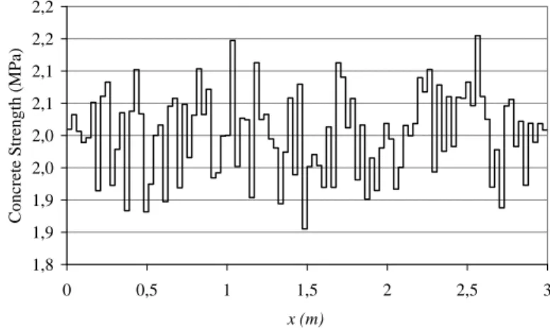
_sst given in Table 1). Concrete is represented by a softening law, using an isotropic plastic model illustrated on Figure 11 (Table 2). To represent the heterogeneity of concrete properties and in order to localize the mechanical degradation, a scattered distribution of the concrete strength



_cst is chosen. Figure 12 represents the evolution



_cst along concrete (from x = 0 to x = 3m). The average strength

st med c ,



and the standard deviation



_y are given in Table 3.

Strain Stress st c







c

E

u



Strain Stress st c







c

E

u



1,8 1,9 1,9 2,0 2,0 2,1 2,1 2,2 2,2 0 0,5 1 1,5 2 2,5 3 x (m) Con crete St reng th (M Pa)

Figure 11 : Form of the softening concrete law

Figure 12 : Distribution of the strength values along the tie

s

E

(GPa)

S

_s (m2₎ st s



(MPa)

210 7.854*10-5 ₄₀₀

Table 1 : Steel parameters (

S

_sis the cross section of steel)

c

E

(GPa)

S

_c (m2₎



u

30 10-2 _0.045%

10

st med c ,



(MPa)



_y (MPa) 2 0.03*



c ,stmed

Table 3 : parameters of the scattered distribution

The bond stress-slip law is represented by a linear function (





k

_b

*

s

where

k

_b is equal to 1010

Pa.m-1₎

III.2 Global mechanical behavior

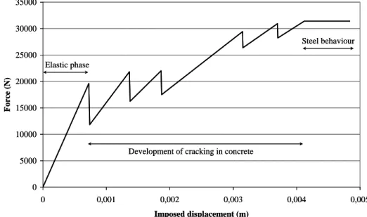
Figure 13 represents the global behavior of the tie. This curve can be divided in 3 parts: - An elastic phase where the behavior of both materials remains linear

- A phase of concrete cracking which is characterized by several peaks and drops of force

- A perfect plastic phase where the behavior is only governed by the steel plastic law (constant force) It is to be noted that these 3 phases are representative of the experimental behavior (Mivelaz, 1996).

0 5000 10000 15000 20000 25000 30000 35000 0 0,001 0,002 0,003 0,004 0,005 Imposed displacement (m) Force ( N) Elastic phase

Development of cracking in concrete

Steel behaviour 0 5000 10000 15000 20000 25000 30000 35000 0 0,001 0,002 0,003 0,004 0,005 Imposed displacement (m) Force ( N) Elastic phase

Development of cracking in concrete

Steel behaviour

Figure 13 : Force-displacement curve

In the following sections, each phase is going to be discussed.

III.3 Elastic phase

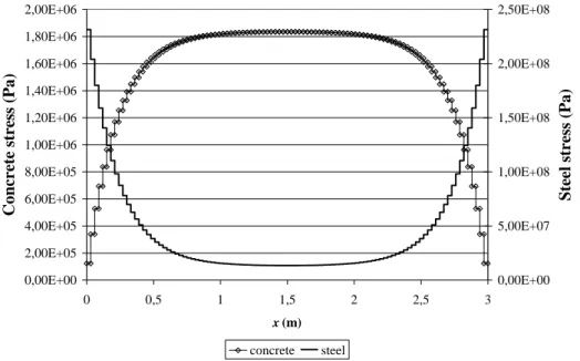
Figure 14 represents an example of stress distribution in both materials along the tie during the elastic phase. As the loading is applied directly on the reinforcement, at each end the force is essentially supported by the steel (

S s

S

F





with



_s the steel stress and F the applied load). Then, in a transition zone, forces are gradually transferred from steel to concrete through the interface: stresses in concrete

11

increase while stresses in steel decrease from the end toward the middle of the tie. Finally, in the central zone, stresses are homogeneous.

0,00E+00 2,00E+05 4,00E+05 6,00E+05 8,00E+05 1,00E+06 1,20E+06 1,40E+06 1,60E+06 1,80E+06 2,00E+06 0 0,5 1 1,5 2 2,5 3 x (m) Co ncrete st ress (Pa ) 0,00E+00 5,00E+07 1,00E+08 1,50E+08 2,00E+08 2,50E+08 St eel st ress (Pa ) concrete steel

Figure 14 : Distribution of the stress along the tie (elastic phase)

To validate the results of the simulation, an analytical resolution is proposed. This solution is obtained from the balance of forces between steel and concrete from a = x to a = L (Figure 15).

F



L

x

a



 

x

F



_s

F



L

x

a



F



L

x

a



 

x

F



_s

Figure 15 : Force balance between a = x and a= L

The external force F applied on steel is balanced by an internal force

F

_s

 

x

and a bond force

 

x

F

_{bond /s} .

 

x

F

 

x

F

F

_s



_bond/s



₍₁₅₎

with, considering the small displacement theory,

 

 

dx x du E S x F s s s s  (16)

12

The bond force

F

_{bond /s}

 

x

is evaluated integrating the bond stress between a = x and a = L. Therefore:

 



_

L



 



 



x c s b s s bond

x

d

k

u

a

u

a

da

F

_/



(17)

where

d

_sis the diameter of the steel bar and

u

_c

 

a

represents the displacement in concrete at a. In the same way, the balance on concrete is given by

 

x



F

_/

 

x



0

F

_{c bond c (18)} with

 

 

dx x du E S x F c c c c  (19) and

 

x

F

 

x

F

_bond/c





_{bond/s (20)}

After development, equations (15) and (18) give the following system:

 

 

 

 























b b s b b a a c s s

S

E

F

dx

x

du

S

E

S

E

dx

x

du

K

dx

x

du

K

dx

x

u

d

2 1 3 3 (21) with



































c c s s b c c s s b

S

E

S

E

F

k

K

S

E

S

E

k

K

2 1

1

1

(22)

After resolution, it comes:

 

 











































  c c x K x K c c s s c x K x K s

S

E

F

K

K

Be

Ae

S

E

S

E

dx

x

du

K

K

Be

Ae

dx

x

du

1 2 1 2 1 1 1 1 (23) where









































_

A

K

K

S

E

F

B

K

K

S

E

F

e

e

e

A

s s s s L K L K L K 1 2 1 2 1 1 1

1

(24)

13

 

 

 

 

















dx

x

du

E

x

dx

x

du

E

x

c c c s s s





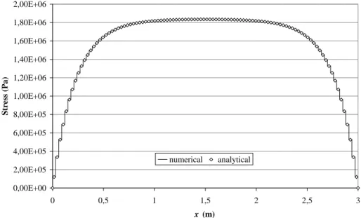
(25)

The numerical results are compared with the analytical solution. Figure 16 represents the stress evolution in concrete along the tie. The results are similar and validate the numerical implementation in this particular case.

0,00E+00 2,00E+05 4,00E+05 6,00E+05 8,00E+05 1,00E+06 1,20E+06 1,40E+06 1,60E+06 1,80E+06 2,00E+06 0 0,5 1 1,5 2 2,5 3 x (m) Stress (P a ) numerical analytical

Figure 16 : Stress distribution in concrete along the tie

III.4 Cracking process

During the elastic phase, the stresses increase in concrete with the imposed displacement. When the strength is reached in a concrete element, an unloading is observed in this element and the stress drops to zero (Figure 17). The load is then fully supported by the corresponding steel element. Its stress becomes equal to

S

S

F

(Figure 18). It is to be noted that this phenomenon is amplified by the use of 1D truss element for concrete. Contrary to what happens in 3D simulation, no evolution of the strain distribution is possible in the concrete cross section. It has nevertheless the advantage to directly highlight the bond effect model on the structural behavior.

When a concrete element is damaged, the stresses are redistributed on each side of the crack. On both sides the stress distribution is similar what was observed during the elastic phase with a gradual transfer from steel to concrete.

14

On a global point of view, the apparition of the first crack coincides with the first partial unloading on the force displacement curve (Figure 13).

0,00E+00 5,00E+05 1,00E+06 1,50E+06 2,00E+06 2,50E+06 0 0,5 1 1,5 2 2,5 3 x (m) Stress (P a )

elastic phase 1st crack distribution of strength

Figure 17 : Distribution of the stress in the concrete along the tie

0,00E+00 5,00E+07 1,00E+08 1,50E+08 2,00E+08 2,50E+08

0,00E+00 5,00E-01 1,00E+00 1,50E+00 2,00E+00 2,50E+00 3,00E+00

x (m)

Stress (P

a

)

elastic phase 1st crack

Figure 18 : Distribution of the stress in the steel along the tie

After the apparition of the first crack, stresses in concrete continue to increase until a tensile strength is reached in a second element. Another crack appears, and a total unloading of the considered element is obtained. The same effect is observed until the steel stress in the cracked zones reaches it yield limit (Figure 19). At this step, the global force cannot increase any more and the distribution of Figure 20 is obtained (5 cracks). The crack length corresponds to the length of one finite element. This effect can

15

be explained by the well-known stress localization due to the use of a softening law. It could be solved by including a regularization technique ((Pijaudier-Cabot and Bazant, 1987) or (Peerlings et al, 2001)). This point will not be discussed in this paper.

0,00E+00 5,00E+07 1,00E+08 1,50E+08 2,00E+08 2,50E+08 3,00E+08 3,50E+08 4,00E+08 4,50E+08

0,00E+00 5,00E-01 1,00E+00 1,50E+00 2,00E+00 2,50E+00 3,00E+00

x (m)

Stress (P

a

)

Yield strength of steel

0,00E+00 5,00E+07 1,00E+08 1,50E+08 2,00E+08 2,50E+08 3,00E+08 3,50E+08 4,00E+08 4,50E+08

0,00E+00 5,00E-01 1,00E+00 1,50E+00 2,00E+00 2,50E+00 3,00E+00

x (m)

Stress (P

a

)

Yield strength of steel

Figure 19 : Stress distribution in the steel at the beginning of the plastic phase

0,00E+00 5,00E+05 1,00E+06 1,50E+06 2,00E+06 2,50E+06 0 0,5 1 1,5 2 2,5 3 x (m) Stress (P a )

final distribution of stress distribution of strength

16

It is to be noted that the crack position is governed, as expected, by the strength distribution but also by the stress evolution imposed by the bond effects. To underline this effect, 10 computations have been carried out considering 10 different distributions of the initial concrete tensile strength.

1 2 3 4 5 6 7 8 9 10 0 0,5 1 1,5 2 2,5 3 x(m) tie number 1 1 1 2 2 2 3 3 3 3 4 4 4 5 5 3 1 2 3 5 4 1 5 2 3 4 5 1 3 2 4 3 3 1 4 2 5 5 2 4 1 3 5 2 3 1 4 2 5 1 4 3

Figure 21 : Position of cracks for the 10 ties. The numbers on the figure correspond to the order of apparition (1 for the first crack until 5 for the fifth crack). The dotted lines correspond to the average

positions of each crack.

Figure 21 shows the crack position along the 10 ties. In most cases (except for one tie), 5 cracks are observed. These cracks are generally localized on one concrete element except when the distribution of strength imposes a simultaneous cracking of two elements (the 3rd _{crack of tie 1 for example). It is}

to be noted that, due to the transfer zone between steel and concrete, no crack can develop at both ends. Finally, the crack spacing is constant with an average value of about 50 cm.

As a conclusion, the order of crack apparition is rather governed by the distribution of the mechanical strength whereas the final state (constant average spacing) is imposed by the stress distribution related to the bond effects.

IV Influence of the bond model

In order to evaluate the influence of the bond effects on the behavior of the tie, the results of the previous simulation are compared with the case where steel and concrete are perfectly bound. In this situation, steel and concrete nodes are identical and the simulation is carried out in the same conditions as described in section III. Figure 22 illustrates the global behavior. It is once again divided in 3 main phases (elastic phase, development of cracking and plastic zone). During the development of cracks, a higher number of partial unloading is observed.

17

0 5000 10000 15000 20000 25000 30000 35000 0 0,001 0,002 0,003 0,004 0,005 0,006 Imposed displacement (m) Force ( N) Steel behaviour

Development of cracking in concrete Elastic phase 0 5000 10000 15000 20000 25000 30000 35000 0 0,001 0,002 0,003 0,004 0,005 0,006 Imposed displacement (m) Force ( N) Steel behaviour

Development of cracking in concrete Elastic phase

Figure 22 : Force-displacement curve at the loaded end of the steel

Figure 23 describes the distribution of stress in both materials during the elastic phase. Contrary to what was observed with the bond model, stresses in steel and concrete are homogeneous along the tie. This can be explained by the perfect relation that imposes an identical strain in both materials. It comes:

F

S

E

S

E

E

F

S

E

S

E

E

c c s s c c c c s s s s













(26) 0,00E+00 2,00E+06 4,00E+06 6,00E+06 8,00E+06 1,00E+07 1,20E+07 1,40E+07

0,00E+00 5,00E-01 1,00E+00 1,50E+00 2,00E+00 2,50E+00 3,00E+00

x (m)

Stress (P

a

)

concrete steel

18

c



increases with the load until the minimal value of the concrete strength is reached. A crack appears in the element. Figure 24 represents the stress distribution in concrete after the first crack. It is to be noted that, with the perfect relation, the stress remains homogeneous in the uncracked concrete. In this zone, the stress can increase until the second concrete strength limit.

Contrary to what was observed with the bond model, the apparition of the cracks is only governed by the strength distribution (Figure 25). At the final state (Figure 26), concrete is totally cracked because the concrete strength has been reached in every element. It explains the high number of partial unloading on the force-displacement curve (Figure 22). The loading is then only supported by steel.

0,00E+00 5,00E+05 1,00E+06 1,50E+06 2,00E+06 2,50E+06

0,00E+00 5,00E-01 1,00E+00 1,50E+00 2,00E+00 2,50E+00 3,00E+00

x (m)

Stress (P

a

)

perfect relation with bond model strength distribution

Figure 24 : Comparison of stress distributions in concrete after the first crack apparition

0,00E+00 5,00E+05 1,00E+06 1,50E+06 2,00E+06 2,50E+06 0 0,5 1 1,5 2 2,5 3 x (m) Stress (P a )

with bond model perfect relation strength distribution

19

0,00E+00 5,00E+07 1,00E+08 1,50E+08 2,00E+08 2,50E+08 3,00E+08 3,50E+08

0,00E+00 5,00E-01 1,00E+00 1,50E+00 2,00E+00 2,50E+00 3,00E+00

x (m)

Stress (P

a

)

concrete steel

Figure 26 : Stress distribution in both materials when concrete is totally cracked (perfect relation)

As expected, the perfect relation is not able to represent the experimental situation where a finite number of cracks is observed. The introduction of the bond effects, as presented in section II, solves this problem.

V Conclusions

In this contribution, a new finite element model is proposed to represent bond effects between steel, modeled with truss elements, and the surrounding concrete. These bond effects are taken into account through additional internal forces calculated from the steel-concrete slip. The proposed model has been applied on a reinforced concrete tie. A characteristic stress distribution has been observed, related to the transfer of bond forces from steel to concrete. In this case, crack apparition is both induced by the heterogeneous characteristics of concrete (distribution of the tensile strength along the tie) and by the transition zones where stresses are redistributed between the materials. At the end of the simulation (mechanical behavior only governed by the steel plastic law), a finite number of crack is observed which corresponds qualitatively to experimental observations (Mivelaz, 1996).

Another simulation, using the hypothesis of a perfect relation between steel and concrete (classical hypothesis used in structural applications) has been also proposed. In this case, the evolution of cracking is only governed by the distribution of the concrete strength since the stresses distribution is homogeneous in uncracked zones. At the final state, the concrete is totally cracked. It shows how the introduction of the bond model can improve the description of the cracking process.

Forthcoming 3D simulations will allow to also evaluate the effects of the stress distribution in the concrete cross section.

20

Even if these results are promising, crack evolution is strongly related to the choice of the bond stress-slip law which has a direct influence on the final number of cracks.

To take this influence into account, an investigation on the bond stress – slip law will thus be launched, based either on literature (Eligehausen et al, 1983), (Kwak and Kim, 2001) or on an experimental campaign to be more representative of the experimental behavior.

Acknowledgements

The authors would like to thank Dr S. Ghavamian for his helpful discussions in the elaboration of the model.

21

References

A. Boulkertous. Interaction feu/Ouvrage en béton armé dans le cas d’un incendie confiné : prédiction de la fissuration. Application de la problématique des installations nucléaires ; Thèse de doctorat de l’ENS Cachan, 2009.

Cast3M. www-cast3m.cea.fr, 2010.

J.L. Clément. Interface acier-béton et comportement des structures en béton armé- Caractérisation- Modélisation. Thèse de doctorat de l’université Paris 6 ; 1987.

A. Daoud. Etude expérimentales de la liaison entre l’acier et le béton autoplaçant – Contribution à la modélisation ; Thèse de doctorat de l’INSA de Toulouse ; 2003.

N. Dominguez. Etude de la liaison Acier-Béton : De la modélisation du phénomène à la formulation d’un Elément Fini Enrichi « Béton Armé » ; Thèse de doctorat de l’ENS de Cachan, 2005.

N. Dominguez, D. Brancherie, L. Davenne, A Ibrahimbegovic. Prediction of crack pattern distribution in reinforced concrete by coupling a strong discontinuity model of concrete cracking and a bond-slip of reinforcement model ; International Journal for Computer-Aided Engineering and Software, vol22, pp558-582, 2005.

R. Eligehausen, E. P. Popov and V.V. Bertero. Local bond stress-slip relationships of deformed bars under generalized excitations, University of California, Report N° UCB/EERC-83/23, October 1983. Eurocode 2. Calcul des Structures en béton, NF-EN-1992, 2007.

H.G. Kwak, S.P.Kim. Bond-slip behavior under monotonic uniaxial loads; Engineering Structures ; Vol 23; p. 298-309, 2001.

L.N. Lowes, J.P. Moehle, S. Govindjee. Concrete-Steel Bond Model for Use in Finite Element Modeling of Reinforced Concrete Structures; ACI Structural Journal; Vol 101, p. 501-511, July-August 2004.

P. Mivelaz. Etanchéité des structures en béton armé- Fuites au travers d’un élément fissuré ; Thèse de doctorat de L’Ecole Polytechnique Fédérale de Lausanne ; 1996.

G. Monti, F.C. Filippou, E. Spacone. Analysis of Hysteretic Behavior of Anchored Reinforcing Bars ; ACI Structural Journal; Vol 94, p. 248-261, May-June1997.

22

D. Ngo, A.C. Scordelis. Finite Element Analysis of Reinforced Concrete Beams ; ACI Journal ; vol 64, p.152-163, March 1967.

R.H.J. Peerlings, M.G.D. Geers, R. de Borst, W.A.M. Brekelmans. A critical comparison of nonlocal and gradient enhanced softening continua ; International Journal of Solids and Structures, vol 38, p.7723-7746, 2001.

V. Picandet, A. Khelidj, G. Bastian. Effect of axial compressive damage on gas permeability of ordinary and high performance concrete , Cement and Concrete Research, vol31, p. 1525-1532, 2001 G. Pijaudier-Cabot and Z.P. Bazant. Nonlocal Damage Theory ; Journal of Engineering Mechanics, vol 113, p.1512-1533, 1987

B. Richard, F. Ragueneau, C. Cremona, L. Adélaide et J.L. Tailhan. A Three-dimensional steel/concrete interface model including corrosion effects ; Engineering Fracture mechanics, 2010.