HAL Id: hal-01927113
https://hal.inria.fr/hal-01927113
Preprint submitted on 19 Nov 2018
HAL is a multi-disciplinary open access
archive for the deposit and dissemination of
sci-entific research documents, whether they are
pub-lished or not. The documents may come from
teaching and research institutions in France or
abroad, or from public or private research centers.
L’archive ouverte pluridisciplinaire HAL, est
destinée au dépôt et à la diffusion de documents
scientifiques de niveau recherche, publiés ou non,
émanant des établissements d’enseignement et de
recherche français ou étrangers, des laboratoires
publics ou privés.
An a priori anisotropic Goal-Oriented Error Estimate
for Viscous Compressible Flow and Application to Mesh
Adaptation
A. Belme, F. Alauzet, A. Dervieux
To cite this version:
A. Belme, F. Alauzet, A. Dervieux. An a priori anisotropic Goal-Oriented Error Estimate for Viscous
Compressible Flow and Application to Mesh Adaptation. 2018. �hal-01927113�
An a priori anisotropic Goal-Oriented Error Estimate
for Viscous Compressible Flow and Application to Mesh Adaptation
A. Belmea,⇤, F. Alauzetb, A. Dervieuxc
aSorbonne Universit´es, UPMC Univ Paris 06, CNRS, UMR 7190, Institut Jean le Rond d’Alembert, 75005 Paris, France
bINRIA Saclay Ile-de-France, Projet Gamma3, 1, rue Honor d’Estienne d’Orves, 91126 Palaiseau, France
cINRIA, Projet Ecuador, 2004 route des lucioles - BP 93, 06902 Sophia Antipolis Cedex, France
Abstract
We present a goal-oriented error analysis for the calculation of low Reynolds steady compressible flows with anisotropic mesh adaptation. The error analysis is of a priori type. Its central principle is to express the right-hand side of the error equation, often referred as the local error, as a function of the interpolation error of a collection of fields present in the nonlinear Partial Di↵erential Equations. This goal-oriented error analysis is the extension of [39] done for inviscid flows to laminar viscous flows by adding viscous terms. The main benefits of this approach, in comparison to other error estimates in the literature, is that the optimal anisotropy of the mesh directly appears in the error analysis and is not obtained from an ad hoc variable nor a local analysis. As a consequence, an optimum is obtained and the convergence of the mesh adaptive process is very fast, i.e., generally the convergence is obtained after 5 to 10 mesh adaptation cycle. Then, using the continuous mesh framework, an optimal metric is analytically obtained from the error estimation. Applications to mesh adaptive calculations of flows past airfoils are presented. Keywords: Viscous compressible flow, goal-oriented mesh adaptation, anisotropic mesh adaptation, adjoint, metric
1. Introduction
Mesh adaptation progressively plays an increasing role in high-fidelity simulation. Beside the direct quantitative expectations, like an increased accuracy, and an higher efficiency for a given error, an important motivation in the extension of mesh adaptation is the better control of error convergence, for example by a better numerical convergence order, since anisotropic mesh adaptation is known as yielding such progress, see [40,57].
The case of Navier-Stokes flows takes a particular place since, due to well identified and localized boundary layers, the researcher and the engineer have early managed for concentrating and as far as possible stretching the mesh near the no-slip boundary. However, already for moderate Reynolds number, the automatic mesh adaptation for Navier-Stokes flows, while not a crucial issue, remains a non-trivial task. A major difficulty is the choice of an error measure.
Many researchers have chosen to focalize on the interpolation error committed on the unknown(s) or on several user-prescribed sensors depending on the unknowns. Mesh adaptation based on P1interpolation error estimate is referred as Hessian-based mesh adaptation. Most works tend to equidistribute the error which consists in minimizing the maximum of the interpo-lation error. Pioneering works have shown a fertile development of Hessian-based and metric-based methods [9,12,22,26,29,
30,34,46,47,52]. In contrast to these equidistribution methods, the “multiscale” variant relies on the optimization of a Lpnorm of the interpolation error [2,36]. The Lpformulation allows the mesh adaptive process to approximate discontinuous solutions with higher-order convergence [40]. However, these methods are limited to the minimization of some interpolation errors for some solution fields, the “sensors”. If for many applications, this simplifying standpoint is an advantage, there are also many applications where Hessian-based mesh adaptation is far from optimal regarding the way the degrees of freedom are distributed in the computational domain. Indeed, Hessian-based methods aim at controlling the interpolation error but this purpose is not often so close to the objective that consists in obtaining the best approximate solution of the PDE. Further, in many engineering applications, one (or several) specific scalar output needs to be accurately evaluated, e.g. lift, drag, or heat flux. Hessian-based mesh adaptation methods are not designed to address this issue.
⇤Corresponding author
A generation of a posteriori error estimates has renewed the existing answers to that issue. A posteriori error estimates take the generic form:
H 7! E(uh) ⇡ Eexact(u uh) ,
where uh = uh(H) is the discrete solution obtained using mesh H. In the Dual Weighted Residual (DWR) method (see [8]), an important element is introduced, the functional error, which carries a mathematical formulation of the purpose of the mesh adaptation e↵ort. Let u, uh, u⇤be the state, the discrete state, and the adjoint state such that
a(u, ') = ( f, ') ; a(uh, 'h) = ( f, 'h) ; a( , u⇤) = (g, ) , the DWR method starts with:
Eexact(u uh) = (g, u uh) = ( f, u⇤ ⇧hu⇤) a(uh,u⇤ ⇧hu⇤) ,
where ⇧h is the P1interpolation operator on mesh H. We observe that the right-hand side is zero if uh solves the continuous equation, or if u⇤is affine, or both. By decomposing the integrals over mesh elements and applying a Green formula, the DWR method identifies the local error which the mesh update will attempt to make uniform. Another way is to evaluate the local error with a finer mesh or by increasing the order of the numerical scheme. These goal-oriented methods have been developed in a series of papers, see e.g. [8,28,31,33,48,53,54,55,56].
However, the initial form of the DWR method does not give a good access to anisotropic mesh adaptation. This difficulty has been circumvented by combining the DWR method and interpolation error criteria as in [53]. It can also be solved by introducing local deformation maps as in [24,23]. It is also addressed in [56], where it is proposed to perform a “what if” study which re-evaluate locally the error after an anisotropic division has been applied to an element. The resulting information is then projected into an anisotropic refinement criterion involving a stretching direction and anisotropy strength. Such approaches are only locally optimal, they do not provide a global optimum. As a consequence, the adaptive process may require a large number of iterations. Our proposal relies on a priori estimates. An a posteriori estimate depends on the mesh through the discrete solution. In contrast, an a priori estimate is expressed directly as a function of the mesh and of the continuous solution u. Typically, it writes:
H 7! E(u, H) ⇡ Eexact(u uh).
A blemish of a priori error estimates is the fact that the main ingredients in right hand-side are high-order derivative (the order is higher than or equal to the order of the equation) of the continuous solution which is unknown. A typical example of mesh adaptation method based on a priori error estimate is the very popular family of Hessian-based methods, also called feature-based mesh adaptation, using estimates such as:
ku uhkL2 C h2kukH2.
Many strategies have been developed to evaluate these second derivatives from the discrete solution uh such as the L2
-projection method [20,26], least-square methods, patch recovery process [58,59], hierarchical approaches [7], ... All these approaches are equivalent to reconstruct a higher-order solution from the piecewise linear discrete solution. Math-ematically Hessian reconstruction methods converge at zeroth order, nevertheless in practice super-convergence appears and a higher rate of convergence is obtained. Even if we can find very specific exemple where some methods do not converge, these approaches are very robust and have been intensively validated in the context of mesh adaptation by the numerous studies that have been published on the subject.
In compensation, these techniques have some attracting features. Among them, we remark that for a scalar error (goal oriented formulation), the mesh adaptation problem can be expressed as an inverse problem (u fixed):
Find Hopt such that E(u, Hopt) = min
H (E(u, H)). (1)
In Problem (1), it is mandatory that the “min” is sought in a set of meshes enjoying some compactness in order to have a well-posed inverse problem. At least, the number of degrees of freedom of the meshes of this set has to be bounded. But, a second important feature of a priori estimates is that we can specify in a more detailed way the class of considered meshes, imposing some regularity, which will lead to a more accurate error analysis. Lastly, the right-hand side of the a priori estimate which we propose here is somewhat dual to the DWR one. Indeed, it writes:
Eexact(u uh) = (g, u uh) = a(⇧hu u, u⇤h) + (g, u ⇧hu) , (2) where u⇤
his the discrete adjoint state. We observe that the error is zero for an affine exact solution: this is the P1-exactness. In contrast to the DWR method, this formulation gives the priority to the reduction of the interpolation error for the state variables.
Right hand-side of Relation (2) involves derivatives of ⇧hu u leading to a H1 analysis of the interpolation error which is much more complex. However, due to the scalar (i.e., integral) form of the functional, integration by parts combined with a smoothness assumption for the adjoint solves this obstacle. Indeed, using integration by part, derivatives can be transposed onto the adjoint state to obtain interpolation errors in L1norm weighted by derivatives of the adjoint state. It is then possible to apply the interpolation error theory to get a majoration of the error. It is also possible to consider the continuous mesh framework [37,38] to derive the optimal mesh minimizing the considered error for a given number of vertices. This gives an optimal answer to Problem (1). This stresses the central role of Pk-exactness of the approximation: if the above interpolation error vanishes, then the approximation error is also zero. And, according to the standard finite element analysis, if the H1norm of this interpolation error is small, so is the approximation error (in the same norm).
The first contribution of this paper is to propose an adjoint-based a priori analysis for elliptic models. A preliminary formu-lation of this analysis was given in [10]. It was tested for elliptic models in [15]. In the present paper, we establish in a more direct manner the error estimation for the elliptic terms.
The second contribution is to extend this analysis to the complete compressible Navier-Stokes system, which involves non-linear parabolic terms. We can demonstrate by manipulating the non-non-linear viscous terms that each of them can be written as a combination of an elliptic terms (on which the above mentioned error estimation applies) and higher order error terms (that can be neglected). By addressing viscous terms, this analysis complements the previous inviscid analysis performed for the compressible Euler equations [39].
The paper is outlined as follows. Section2recalls the continuous mesh framework which provides a duality between discrete meshes and entities and Riemannian metric space and metric tensor. The continuous interpolation error local model is also provided. Section3proposes a new a priori estimate for the Poisson problem. Then, Section4gives the Navier-Stokes system for compressible gas and the considered variational discrete formulation. The goal-oriented error estimate for the Navier-Stokes equations is given in Section5, and Section6formulates the mesh optimization problem leading to the expression of the optimal continuous mesh. Finally, Section7 states how the optimal discrete meshes is obtained and Section 8 gives few numerical experiments illustrating the optimality of the proposed adaptation process.
2. Continuous mesh model
We propose to work in the continuous mesh framework introduced in [37,38]. The main idea of this framework is to model discrete meshes by continuous Riemannian metric fields. In that context, a continuous meshM of computational domain ⌦ ⇢ Rd is identified to a Riemannian metric field (M(x))x2⌦. It defines proper di↵erentiable optimization [6], in other words calculus of variations can be used on continuous meshes while it cannot be applied on discrete meshes. For d = 3 and anyx of ⌦, M(x) is a symmetric 3 ⇥ 3 matrix having ( i(x))i=1,3as eigenvalues along the principal directions R(x) = (vi(x))i=1,3. Metric tensor M(x) is a continuous element modeling discrete element K (triangle in 2D and tetrahedron in 3D). For i = 1, 3, sizes along principal directionsvi(x) are given by hi(x) =
1 2
i (x) and anisotropy quotients riare defined by: ri=h3i(h1h2h3) 1. Anisotropic quotient represent the anisotropy of the continuous element. The diagonalisation of M(x) writes:
M(x) = d23 M(x) R(x) 0 BBBBB BBBBB BB@ r 23 1 (x) r 23 2 (x) r 23 3 (x) 1 CCCCC CCCCC CCA tR(x) . (3)
The continuous mesh density dM(x) at node x is equal to: dM = (h1h2h3) 1 = ( 1 2 3)12 = pdet(M). By integrating it, we define the continuous mesh complexity C(M):
C(M) = Z ⌦ dM(x) dx = Z ⌦ p det(M(x)) dx ,
which enables the user to control the level of accuracy of the mesh, and thus, to implicitly control the number of vertices of the resulting discrete mesh.
The main idea of metric-based mesh adaptation, initially introduced in [27], is to generate a unit mesh in the prescribed Riemannian metric spaceM, e.g. a mesh of ⌦ ⇢ Rdsuch that each edgee has a unit length and each element K - tetrahedron or triangle - is regular (or equilateral) with respect to (M(x))x2⌦:
8e, `M(e) = 1 and 8K, |K|M= p 3 4 in 2D or |K|M = p 2 12 in 3D ,
where the length of edgee = ab with respect to M is computed using the straight line parameterization (t) = a + t ab, where t 2 [0, 1]: `M(ab) = Z 1 0 k 0(t)k M dt = Z 1 0 q abT M(a + t ab) ab dt , and the volume of element K with respect toM is:
|K|M= Z
K p
det M(x) dx .
The resulting discrete mesh in the canonical Euclidean space will be anisotropic and adapted. We want to emphasize that the set of all the discrete meshes that are unit meshes with respect to a unique continuous meshM contains an infinite number of discrete meshes.
Given a smooth function u defined on ⌦, to each unit mesh H with respect to continuous mesh M corresponds a local discrete interpolation error |u ⇧hu| on each element. In [37,38], it is shown that all these interpolation errors are well represented by the continuous interpolation error related toM which is locally expressed in term of the Hessian Huof function u as follows:
|u ⇡Mu|(x) = cd trace⇣M 12(x) |Hu(x)| M 12(x)⌘ , (4) where cdequals 18in 2D and 201 in 3D, and |Hu| is deduced from Huby taking the absolute values of its eigenvalues.
Remark 2.1. The above metric density dMis generally a smooth function representing the discrete vertex density dH of the unit mesh H with respect to M. In contrast, the density dH is a sum of Dirac located at vertices and can be therefore considered as highly oscillating. The metric density is a homogenization of the unit mesh density. Indeed, a continuous mesh convergent sequence can be defined according to the continuous mesh complexity C(M) = N and a reference metric M1of complexity equal to one C(M1) = 1:
MN =C(M) M1=N M1, N ! 1 .
To fix the idea, we can consider an average mesh size h corresponding to complexityN, and reformulate the continuous mesh convergent sequence as:
Mh=h dM1, h ! 0 ,
where d is the domain dimension. The continuous and discrete densities are close to each other in the sense that: 8 2 D(⌦), (dMN, ) (dHN, ) ! 0 as N ! 1 ,
where HNis a unit mesh for MN, and D(⌦) is the subset of C1( ¯⌦) functions with compact support. Similarly, given a smooth function u defined on ⌦, and its P1interpolation ⇧
hu on unit mesh H for Mh, the interpolation error u ⇧hu is also a highly oscillatory function. Now, according to [37,38], it is possible to homogenize the discrete interpolation error using the continuous interpolation error of Relation (4) expressed in terms of the Hessian Hu of u in such a way that, for h ! 0,
|u ⇧hu| = h2ehomoginterp(u) + h2eoscillinterp(u) + h2o(h)L2(⌦) with ehomoginterp(u) = |u ⇡M1u| where ehomoginterp(u) is the homogenized interpolation error, h2o(h)
L2(⌦)is an error term of order strictly higher than two according to L2analysis, and h2eoscill
interp(u) is the oscillatory component of the interpolation error which is also a error term of order strictly higher that two since eoscill
interp ! 0 in D0(⌦). 3. A priori finite-element analysis
Standard a priori estimates have been early derived in H1(⌦) (“projection property”), and in L2(⌦) (Aubin-Nitsche analysis), but only by means of inequalities. Moreover, the leading term of the error is generally not exhibited (only bounds of it are proposed). In this section, we go a little further in the Aubin-Nitsche a priori analysis to be able to consider the continuous mesh framework and to be able to exhibit the optimal adapted mesh such as in [11,39]. To this end, we consider an important simplification in the analysis by neglecting the boundary error terms. It has already been done and discussed in previous works [39]. In short, this is possible because in our type of approximation, close to FEM, the accuracy of the boundary discretization can degrade of one order of accuracy without changing the asymptotic convergence in H1(⌦) or L2(⌦). This simplification avoids to generate adapted meshes which would be strongly inhomogeneous close to boundaries which may degrades numerical scheme stability and accuracy. In this section, we focus on the Poisson problem which is set on domain ⌦ ⇢ Rd:
u = f on ⌦ ; u = 0 on @⌦ . (5)
Its variational form writes:
a(u, v) =Z
⌦ru.rv dx = ( f, v) , 8 v 2 V ,
(6) where V holds for the Sobolev space V = H1
0(⌦) = u 2 L2(⌦), ru 2 (L2(⌦))d,u|@⌦ =0 . In order to derive an a priori estimate, we assume that solution u has some extra smoothness:
u 2 V = V \ C3( ¯⌦).
where C3( ¯⌦) is the set of functions of class C3 on ⌦ [ @⌦. Let H be a mesh of ⌦ made of simplices (triangles in 2D and tetrahedrons in 3D): H =SkKk. Let Vhbe the subspace of V of continuous functions that are P1on each element of the mesh:
Vh = n
'h 2 V 'h|K is affine 8K 2 H o
. The discrete variational problem is then defined by:
a(uh,vh) = ( f, vh) , 8 vh2 Vh. (7) Let us introduce the linear interpolation operator ⇧hfrom vertices values:
⇧h: V ! Vh ; u 7! ⇧hu such that ⇧hu|K is affine 8K 2 H and ⇧hu(x) = u(x) , for all vertices x of mesh H . In a goal-oriented analysis, we are interested in estimating (g, uh u) which can be split into two components:
(g, uh u) = (g, uh ⇧hu) + (g, ⇧hu u) , (8) where we recognize in the second di↵erence ⇧hu u the interpolation error, and the first di↵erence uh ⇧hu is referred as the implicit error. Introducing the continuous and the discrete adjoint states u⇤and u⇤
hverifying: a( , u⇤) = (g, ) , 8 2 V and a(
h,u⇤h) = (g, h) , 8 h 2 Vh, we get
(g, uh u) = a(uh ⇧hu, u⇤h) + (g, ⇧hu u) . (9) The second term of the right hand-side can be estimated without any difficulty using Relation (4) :
|(g, ⇧hu u)| Z ⌦|g| |u ⇧ hu| d⌦ Z ⌦ cd|g| trace⇣M 12|Hu| M 12⌘d⌦ , while it would have been a lot more complicated using the equality:
(g, ⇧hu u) = a(⇧hu u, u⇤) .
Analyzing the first term of the right hand-side of Relation (9) comes to study the following term: a(uh ⇧hu, ⇧h') ,
where ' is any sufficiently smooth function. To this end, we first express the implicit error term as a function of the interpolation error. It is useful to remark that the discrete statement is equivalently written:
a(uh, ⇧h') = ( f, ⇧h') , 8 ' 2 V. (10) Using Relation (10) and then Relation (6), we get:
a(uh ⇧hu, ⇧h') = a(uh, ⇧h') a(⇧hu, ⇧h') = ( f, ⇧h') a(⇧hu, ⇧h') = a(u, ⇧h') a(⇧hu, ⇧h') , (11) which gives:
a(uh ⇧hu, ⇧h') = a(u ⇧hu, ⇧h') , 8 ' 2 V. (12) Note that u ⇧hu is not solution of the discrete adjoint system because u is not in Vh. Therefore, we propose the following main result:
Lemma 3.1. For any couple of smooth functions (u, '), where u is not necessarily a solution of Problem (5), we have the following bounds: | Z ⌦ @ @xi(u ⇧hu) @ @xj⇧h'd⌦| Kd Z ⌦| ⇢ H(')| |u ⇧hu| d⌦ + BT | Z ⌦ @ @xiu(u ⇧hu) @ @xj⇧h'd⌦| Kd Z ⌦| ⇢ H(')| |u| |u ⇧hu| d⌦ + BT
where Kd = 3 in two dimensions, Kd = 6 in three dimensions, and A B holds for a majoration asymptotically valid, i.e. A B + o(A) when mesh size tends to zero. Expression | ⇢H(') | holds for spectral radius of H(') which is the Hessian of ', i.e., the largest (in absolute value) eigenvalue of H('). The boundary terms BT are not used in the sequel.
To prove this result, we analyze the right-hand side term of Equality (12): a(u ⇧hu, ⇧h') = Z ⌦r(u ⇧ hu) · r⇧h'd⌦ = X K2H Z Kr(u ⇧hu) · r⇧h'dK ,
where the sum ⌃ is taken over any element K of mesh H. As the aim is to extend this analysis to the Navier-Stokes equations, we analyze the following generic integral term (in which index i is not necessary equal to index j contrary to the Poisson problem):
I = X K2H Z K @ @xi(u ⇧hu) @ @xj⇧h' ! dK = X K2H Z @K(u ⇧hu) @ @xj⇧h' ! nK xid Z K(u ⇧hu) @2 @xi@xj⇧h' ! dK ! , after integration by parts, and, as ⇧h'is linear over K, it reduces to:
I = X K2H Z K @ @xi(u ⇧hu) @ @xj⇧h' ! dK = X K2H Z @K(r⇧h') |K· ejn K xi(u ⇧hu) d . where (ej)j=1..dstands for the canonical basis of Rd, and nKxiis the i
thcomponent of unit outward normalnK =(nK x1,n K x2,n K x3) T to the element boundary. As stated above, boundary integrals on @⌦ do not contribute to the volume estimate and are thus discarded in our analysis. The above integral can also be written as an integral over the edges in 2D or the faces in 3D of the mesh. Hence, to develop further this analysis, we consider the integral on the edge or the face sharing the two neighboring triangles or tetrahedrons K+and K . Thanks to the continuity of u ⇧hu, it writes:
I = X @K+\@K Z @K+\@K ⇥(r⇧h') |K+ (r⇧h') |K ⇤ · ejn K+ xi (u ⇧hu) d , where nK+ xi is the ith component of nK+ = (n K+ x1 ,n K+ x2 ,n K+
x3 )T the unit normal to the considered edge/face. Introducing the following notation for the jump of the '-derivative over the edge/face:
⇥r⇧h'⇤+ =⇥(r⇧h') |K+ (r⇧h') |K ⇤,
we observe that the gradient component of ⇧h'in directiontK+ tangent to the common edge/face is continuous, therefore we have:
⇥r⇧h'⇤+ · t K+ =0 , from which we deduce the following relations with the unit edge/face normal:
⇥r⇧h'⇤+ = ⇥r⇧h' ⇤ + nK+ and ⇥r⇧h' ⇤ + =⇥r⇧h' ⇤ + · nK+ . From the above relations, we get:
⇥r⇧h'⇤+ · ej = ⇥r⇧h' ⇤ + n K+ xj = ⇥r⇧h' ⇤ + · n K+ nK+ xj , and, finally, we obtain:
⇥r⇧h'⇤+ · ejn K+ xi = ⇥r⇧h' ⇤ + · n K+ nK+ xj n K+ xi . Thus, the above integral becomes:
I = X @K+\@K Z @K+\@K ⇥(r⇧h') |K+ (r⇧h') |K ⇤ · n K+ nK+ xj n K+ xi (u ⇧hu) d , 6
G_ G+ e A C B C' T_ T+ A B C D D’ f G+ G_ T+ T_
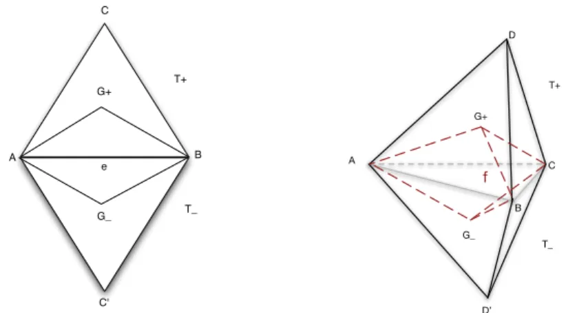
Figure 1: Super-convergent molecule for a vertical derivative. Diamond decomposition of the mesh over each edge in 2D (left) and each face in 3D (right).
Now, we can provide a first upper bound: |I| = Z ⌦ @ @xi(u ⇧hu) @ @xj⇧h' ! d⌦ X @K+\@K ⇥(r⇧h') |K+ (r⇧h') |K ⇤ · n K+ Z @K+\@K |u ⇧hu| d ,
To pursue our analysis, this integral can be transformed into an integral over ⌦ by considering a diamond cell partitioning: H = SkKk = SiDi, where each diamond cell Di is associated to an edge e in 2D or a face f in 3D. In two dimensions, a diamond cell Deassociated to an edge e is the union of the two sub-triangles that are build by joining the centers of gravity of the two triangles sharing the edge e to the edge e, see Figure1(left). In three dimensions, a diamond cell Df attached to a face f is the union of the two sub-tetrahedrons that are build by joining the centers of gravity of the two tetrahedrons sharing the face f to the face f , see Figure1(right). If we denote by | · | the measure (length, area, volume) of geometric entity and h the height of a simplex K, by definition, we have the following relations for the area in 2D:
|De| = |K+| + |K | 3 =|e|
|h+| + |h |
6 , (13)
and for the volume in 3D:
|Df| =|K+| + |K | 4 =| f ||h
+| + |h |
12 . (14)
Moreover, taking the mean of |u ⇧hu| over the edge e = @K+\ @K or the face f = @K+\ @K is a consistent quadrature for the integration of |u ⇧hu| over the diamond cell D+ , thus:
1 |@K+\ @K | Z @K+\@K |u ⇧hu| d ⇡ 1 |D+ | Z D+ |u ⇧hu| dD+ , (15)
And finally, we observe that the term:
⇥(r⇧h') |K+ (r⇧h') |K ⇤ · n
K+ = @
@nK+⇧h'|K+ @ @nK ⇧h'|K
appears as a second derivative of ' in the normal direction to the edge/face weighted by the inverse of the average height of the two neighboring simplex. If we introduce | ⇢H(') | the spectral radius of H(') which is the Hessian of ', the spectral radius being the largest (in absolute value) eigenvalue of H('), we get the following bound:
⇥(r⇧h') |K+ (r⇧h') |K ⇤ · n
K+ |h+| + |h |
2 | ⇢H(')| . (16)
In two dimensions, using Relations (13), (15), and (16), we obtain the following upper bounds:
|I| X @K+\@K ⇥(r⇧h') |K+ (r⇧h') |K ⇤ · n K+ Z @K+\@K |u ⇧hu| d X e2H |h+| + |h | 2 | ⇢H(')|! 0BBBBB@ |e| |e||h+|+|h | 6 Z De |u ⇧hu| dDe 1 CCCCC A ,
and after canceling terms, we finally obtain: |I| X e2H 3 | ⇢H(')| Z De |u ⇧hu| dDe=3 Z ⌦| ⇢ H(')| |u ⇧hu| d⌦ , in 2D .
Similarly, in three dimensions, using Relations (14), (15), and (16) and canceling terms, we obtain the following upper bounds:
|I| X f 2H 6 | ⇢H(')| Z Df |u ⇧hu| dDf =6 Z ⌦| ⇢ H(')| |u ⇧hu| d⌦ , in 3D .
The same demonstration holds if we replace the term (u ⇧hu) by the term u (u ⇧hu). This concludes the proof of the Lemma
3.1. The estimate of Lemma3.1has been successfully tested for mesh adaptation in [13] and also compared with another estimate in [14].
4. Navier-Stokes Model 4.1. Continuous state system
The steady compressible Navier-Stokes system for a perfect gas is set in computational domain ⌦ ⇢ R3and can be written under a compact form as:
r · FE(W) + r · FV(W) = 0 on ⌦ (17)
where W =t(⇢, ⇢u, ⇢E) is the conservative flow variables vector and vector FErepresents the Euler fluxes: FE(W) =t(⇢u, ⇢u
1u + pe1, ⇢u2u + pe2, ⇢u3u + pe3, ⇢uH) .
We have noted ⇢ the density,u = (u1,u2,u3) the velocity vector, H = E + p/⇢ is the total enthalpy, E = T +kuk 2
2 the total energy and p = ( 1)⇢T the pressure with = 1.4 the ratio of specific heat capacities, T the temperature, and (e1,e2,e3) the canonical basis.
We describe in short the viscous fluxes and viscous stress tensor as follows: FV(W) = [0, , (q u. )]T ; = µ(ru + ruT) 2
3µr.uI,
with µ representing the constant viscosity. The heat fluxq is given by Fourier’s law q = rT, where is the heat conduction (assumed here to be constant). The five unknowns are gathered in functional product space (we use the same notation):
V = hH1(⌦) \ C3( ¯⌦)i⇥hH1
0(⌦) \ C3( ¯⌦) i3
⇥hH1(⌦) \ C3( ¯⌦)i, (18) assuming adiabatic conditions on walls. We formulate the Navier-Stokes model in a compact variational formulation:
Find W 2 V such that 8 2 V, ( (W) , ) = 0 with = E+ + V, (19) where =⇣ ⇢, ⇢u1, ⇢u2, ⇢u3, ⇢E
⌘T
. The Euler term Erelies on the usual Euler fluxes FE: ⇣ E
(W) , ⌘ = Z
⌦ · r · F
E(W) d⌦. (20)
Term holds for boundary fluxes contribution which we denote shortly: ⇣
(W) , ⌘ = Z
· ˆF (W) · n d . Viscous fluxes FVprovide seven terms:
( V(W), ) =Z ⌦ · r · F V(W) d⌦ =X7 k=1 TV k . (21) 8
The first three terms come from moment equations and depend only on ⇢u=( ⇢u1, ⇢u2, ⇢u3)T: TV 1 = Z ⌦ ⇢u· r · (µru) d⌦ TV 2 = Z ⌦ ⇢u· r · ⇣ µ(ru)T⌘d⌦ TV 3 = 23 Z ⌦ ⇢u· r · (µ (r · u) I) d⌦ . The last four terms are derived from the energy equation:
TV 4 = Z ⌦ ⇢Er · ( rT) d⌦ TV 5 = Z ⌦ ⇢Er ·⇣µu · (ru)T⌘d⌦ TV 6 = Z ⌦ ⇢Er · (µ u · ru) d⌦ TV 7 = 23 Z ⌦ ⇢Er · (µ u · ((r · u) I)) d⌦ . 4.2. Variational discrete formulation
For the spatial semi-discrete model, we consider the mixed Finite Element - Finite Volume formulation [21,45]. As in [39], we reformulate it under the form of a finite element variational formulation. We assume that ⌦ is covered by a unit mesh H with respect to a given Riemannian metric spaceM = (M(x))x2⌦composed of simplicial elements, denoted K. Let us introduce the following approximation space:
Vh = n h2 V h|K is affine 8K 2 Ho , where V is defined by Relation (18). (22) The weak discrete formulation writes:
Find Wh2 Vh such that 8 h2 Vh, h(Wh) , h =0, with h(Wh) , h = Z ⌦ h· r · F E h (Wh) d⌦ Z h· ˆFh(Wh).n d + Z ⌦ h· r · F V h (Wh) d⌦ + Z ⌦ h· D h(Wh) d⌦ . (23) The fourth term in Formulation (23) is an added numerical di↵usion dedicated to numerical stability. In short, the Dh term involves the di↵erence between the Galerkin central-di↵erences approximation and a second-order Godunov approximation defined as in [21]. In the present study, we only need to know that for smooth fields, the Dh term is a third-order term with respect to the mesh size parameter h and will not be considered in our estimate.
Taking in System (23) the P1interpolation of the fluxes F as discretization principle, produces a finite-element scheme which is identical to the central-di↵erenced finite-volume scheme built on the so-called median dual cells [45], thus:
8 W 2 Vh[ V , FhE(W) = ⇧hFE(W) and ˆFh(W) = ⇧hF (W) .ˆ (24) However, concerning the viscous term, we cannot apply a similar treatment because we have fluxes of order two (second deriva-tives) and we cannot apply directly the interpolation operator. Let f be the transformation function from primitive variables U = (⇢,u, T) into conservatives ones W = (⇢, ⇢u, ⇢E), we set:
FhV(W) = FhV( f (U)) = FV( f (⇧hU)) = FV( f (⇧hf 1(W))).
In other words, our discretization consists of P1interpolating the primitive variables in the above viscous terms {TV
i }i=1..7for our discretization principle. This completes the definition of the discrete system under study.
4.3. Mesh adaptation : discrete problem statement
Let g be a function of V. We assume that the purpose of the numerical problem is to evaluate the output functional: j = (g, W) where W is the solution of Problem (19).
The problem addressed in this paper is to find the discrete mesh which minimizes the following functional error given a fixed number of vertices N:
j = (g, W Wh) where W is the solution of Problem (19) and Wh is the solution of Problem (23). The next sections are devoted to this error analysis and the optimal formulation of the mesh adaptation problem.
5. Error analysis for Navier-Stokes problem
The Navier-Stokes equations are a non-linear system, thus some extra justifications are required to be able to perform an error analysis similar to the linear case (done in Section3). The following justify why it is possible to apply a similar analysis in the non-linear case.
Let be a smooth test function of V defined in Relation (18). Let W be the solution of Problem (19) and Whthe solution of Problem (23), the continuous and discrete state equation write:
( (W) , ) = 0 and ( h(Wh) , ⇧h ) = 0 ,
where ⇧h lies in Vhdefined by Relation (22). We also introduce the continuous and the discrete adjoint states: W⇤and Wh⇤. The continuous adjoint system related to the objective functional writes:
W⇤2 V , 8 2 V : @
@W(W) , W⇤ !
= (g, ) . (25)
From functional analysis theory, a well-posed continuous adjoint system can be derived for any functional output as far as the linearized system is well posed. This however does not mean that any output functional leads to properly defined adjoint boundary conditions. Several works in the literature [4,5,17,19] illustrate this problem and propose solutions, usually by adding auxiliary boundary terms to the Lagrangian functional. In [19], it is concluded that for the compressible Navier-Stokes system, only functionals which involve the entire stress tensor at obstacle boundary are admissible. We assume here that (25) is well-posed and gives a sufficiently smooth continuous adjoint state. The discrete adjoint system writes:
W⇤
h 2 Vh,8 h2 Vh : @ h
@W(Wh) h,Wh⇤ !
= (g, h) . 5.1. Linearized error system
In our error estimation problem presented in Section4.3, the approximation error can be decomposed into an implicit error term and an interpolation error term:
j = (g, W Wh) = (g, W ⇧hW) + (g, ⇧hW Wh) .
The interpolation error can be easily estimated, see Relation (4), while the implicit error is solution of a discrete system that we derive in the following. Now, we assume that Wh can be made close enough to ⇧hW when h ! 0 in such a way that we can identify the main term of the left-hand side as a Jacobian times the di↵erence:
@ h @W(Wh)(Wh ⇧hW) , ⇧h ! ⇡ ⇣ h(Wh) h(⇧hW) , ⇧h ⌘ as h ! 0.
Then, combining continuous and discrete systems, we can write similarly to Relation (11) an equality linking implicit and interpolation errors which is valid for all :
( h(Wh) h(⇧hW) , ⇧h ) = ( h(Wh) , ⇧h ) ( h(⇧hW) , ⇧h ) = ( (W) , ⇧h ) ( h(⇧hW) , ⇧h ) = ( (W) h(⇧hW) , ⇧h )
We are then interested in the following error on functional: |(g, Wh ⇧hW)| ⇡ ⇣ h(Wh) h(⇧hW) , Wh⇤ ⌘ =⇣ (W) h(⇧hW) , Wh⇤ ⌘ . (26)
The right-hand side of the above relation is composed of (see Relation (23)) the Euler term, the Euler boundary term, the viscous term, and the stabilization term. In the following, we neglect the boundary term (as in the previous analysis) and the stabilization term thanks to smoothness of functions W and W⇤. The boundary term analysis is given in [39].
The method proposed here involves some heuristics. In particular, we assume that the interpolate of the adjoint is close to the discrete adjoint:
⇧hW⇤⇡ Wh⇤. Therefore:
|(g, Wh ⇧hW)| ⇡ ( (W) h(⇧hW) , ⇧hW⇤) . 10
5.2. A priori estimate for Navier-Stokes problem
We can now give the main result of this paper which is the following a priori estimate:
Proposition 5.1. Let us assume that W 2 V and 2 V where V is defined by Relation (18) and =⇣ ⇢, ⇢u1, ⇢u2, ⇢u3, ⇢E ⌘T
. Then, we have the following error bound for h sufficiently small:
|( (W) h(⇧hW), ⇧h )| E with: E = Z ⌦| r | · F E(W) ⇧ hFE(W) d⌦ + d +1 3 ! Kd d X i=1 Z ⌦ µ| ⇢H( ⇢ui)| |ui ⇧hui| d⌦ + 1 3Kd d X i=1 d X j=1 j,i Z ⌦ µ| ⇢H( ⇢ui)| |uj ⇧huj| d⌦ + Kd Z ⌦ | ⇢ H( ⇢E)| |T ⇧hT| d⌦ + (d +1 3) Kd d X i=1 Z ⌦ µ| ⇢H( ⇢E)| |ui| |ui ⇧hui| d⌦ + 1 3Kd d X i=1 d X j=1 j,i Z ⌦ µ| ⇢H( ⇢E)| |ui| |uj ⇧huj| d⌦ + 5 3 d X i=1 d X j=1 j,i Z ⌦ µ @(⇧h ⇢E) @xj (uj ⇧huj) @ui @xi (ui ⇧hui) @uj @xi ! d⌦ ,
and Kd = 3 in two dimensions, Kd = 6 in three dimensions, and A B holds for a majoration asymptotically valid, i.e. A B + o(A) when mesh size tends to zero. Expression | ⇢H(') | holds for spectral radius of the Hessian of '.
The proof of this Proposition is given inAppendix A. Le last term of this estimation requires additional manipulations (done in the Appendix) to make its implementation easier. This term is expressed in the following by means of the vector !.
This main result can be written in a more convenient way to facilitate its implementation by gathering interpolation error terms on the primitive variables. Here, we give the 2D and the 3D re-writing of it, using notations introduced inAppendix A. Corollary 5.1. Let us assume that W 2 V and 2 V where V is defined by Relation (18) and =⇣ ⇢, ⇢u1, ⇢u2, ⇢E
⌘T . Then, in two dimensions (Kd=3), we have the following error bound for h sufficiently small:
|( (W) h(⇧hW), ⇧h )| Z ⌦ GFE FE(W) ⇧hFE(W) d⌦ + Z ⌦ Gu1|u1 ⇧hu1| d⌦ + Z ⌦ Gu2|u2 ⇧hu2| d⌦ + Z ⌦ GT|T ⇧hT| d⌦ , with the coefficients:
GFE = | r | Gu1 = µ 7 | ⇢H( ⇢u1)| + | ⇢H( ⇢u2)| + ⇣ 7|u1| + |u2| ⌘ | ⇢H( ⇢E)| +5 3|!u2,z| ! Gu2 = µ | ⇢H( ⇢u1)| + 7 | ⇢H( ⇢u2)| + ⇣ |u1| + 7|u2| ⌘ | ⇢H( ⇢E)| +5 3|!u1,z| ! GT = 3 | ⇢H( ⇢E)|
and the ! vector defined by:
rui⇥ r ⇢E =!ui = ⇣
!ui,x, !ui,y, !ui,z ⌘T
, where only the last component is not zero.
Corollary 5.2. Let us assume that W 2 V and 2 V where V is defined by Relation (18) and =⇣ ⇢, ⇢u1, ⇢u2, ⇢u3, ⇢E ⌘T
. Then, in three dimensions (Kd=6), we have the following error bound for h sufficiently small:
|( (W) h(⇧hW), ⇧h )| Z ⌦ GFE FE(W) ⇧hFE(W) d⌦ + Z ⌦ Gu1|u1 ⇧hu1| d⌦ + Z ⌦ Gu2|u2 ⇧hu2| d⌦ + Z ⌦ Gu3|u3 ⇧hu3| d⌦ + Z ⌦ GT|T ⇧hT| d⌦ , with the coefficients:
GFE = | r |
Gu1 = µ 20 | ⇢H( ⇢u1)| + 2 | ⇢H( ⇢u2)| + 2 | ⇢H( ⇢u3)| + ⇣
20|u1| + 2|u2| + 2|u3| ⌘
| ⇢H( ⇢E)| +5
3|!u3,y !u2,z| !
Gu2 = µ 2 | ⇢H( ⇢u1)| + 20 | ⇢H( ⇢u2)| + 2 | ⇢H( ⇢u3)| + ⇣
2|u1| + 20|u2| + 2|u3| ⌘
| ⇢H( ⇢E)| +5
3|!u1,z !u3,x| !
Gu3 = µ 2 | ⇢H( ⇢u1)| + 2 | ⇢H( ⇢u2)| + 20 | ⇢H( ⇢u3)| + ⇣
2|u1| + 2|u2| + 20|u3| ⌘
| ⇢H( ⇢E)| +5
3|!u2,x !u1,y| ! GT = 6 | ⇢H( ⇢E)|
and the ! vector defined by:
rui⇥ r ⇢E =!ui = ⇣
!ui,x, !ui,y, !ui,z ⌘T
.
For the next section where we seek for the optimal mesh that minimize the above error model, it is useful to note that the error model can be written under the compact form:
|( (W) h(⇧hW), ⇧h )| Z ⌦ X k Gk(µ, , U, r , | ⇢H( )|) Sk(W) ⇧hSk(W) d⌦ , (27) in other words, the error model is a sum of interpolation errors weighted by algebraic functions.
6. Goal-oriented optimal continuous mesh
6.1. Mesh adaptation : continuous problem statement
According to the continuous mesh theory [37,38] presented in Section2, we transform the a priori error estimate of Propo-sition5.1into a continuous error estimate. To this end, the following modifications are done:
• mesh H is replaced by continuous mesh M = (M(x))x2⌦ • number of vertices N is replaced by complexity C(M) = N • the P1projection operator ⇧
hdefined on mesh H is replaced by the P1continuous mesh operator ⇡Mdefined on continuous meshM = (M(x))x2⌦
• discrete interpolation error u ⇧hu defined on mesh H is replaced by continuous interpolation error u ⇡Mu defined on continuous meshM = (M(x))x2⌦.
Then, using Relations (26) and (27), we can reformulate the discrete mesh adaptation problem introduced in Section 4.3in the continuous mesh framework: find the continuous meshMopt which minimizes the following functional error given a fixed complexity N: j = (g, W Wh) ⇡ (g, W ⇧hW) + ( (W) h(⇧hW) , ⇧hW⇤) Z ⌦ X k |gk| Wk ⇡MWk d⌦ + Z ⌦ X k Gk(µ, , U, rW⇤,| ⇢H(W⇤)|) Sk(W) ⇡MSk(W) d⌦ , (28) where W is the solution of Problem (19), Whis the solution of Problem (23) and W⇤is the solution of Problem (25).
As the above relation is a weighted sum of interpolation errors, by introducing the following positive symmetric matrix Hgo(x) = X k |gk| |HWk| + X k Gk(µ, , U, rW⇤,| ⇢H(W⇤)|) |HSk(W)| (29) 12
where |HWk| and |HSk(W)| are the absolute value of the Hessian of fields Wkand Sk(W), and using the definition of the continuous interpolation error given by Relation (4), we can state the following error estimate on continuous meshM = (M(x))x2⌦:
j ⇡ Ego(M) = cd Z
⌦
trace⇣M 12(x) Hgo(x) M 12(x)⌘ d⌦ .
It is then possible to set the well-posed global optimization problem of finding the optimal continuous meshMgo minimizing continuous interpolation errorEgo(M):
FindMgo=min
M Ego(M) under the constraint C(M) = N . (30) 6.2. Optimal goal-oriented continuous mesh
We seek for the optimal continuous meshMgosolution of Problem (30). Similarly to [39], solving the optimality conditions provides the optimal goal-oriented continuous meshMgo =(Mgo(x))x2⌦defined point-wise by:
Mgo(x) = N2d Z ⌦ (detHgo(¯x))d+21 d¯x ! 2 d ⇣ detHgo(x)⌘ 1 d+2 H go(x). (31)
where d is the dimension. The corresponding optimal error writes: Ego(Mgo) = = 3 N 2 d Z ⌦ (detHgo(x)) 1 d+2dx !2+d d , (32)
where the exponent of N illustrates the second-order accuracy of the method. 7. From theory to practice
The continuous mesh adaptation problem takes the form of the following continuous optimality system: W 2 V , 8 2 V , ( (M, W), ) = 0 “Navier-Stokes system” W⇤2 V , 8 2 V , @
@W(M, W) , W⇤ !
=(g, ) “Adjoint system”
M = Mgo “Adapted continuous mesh”. In practice, it is necessary to approximate the above three-field coupled system by the discrete optimality system:
W 2 Vh, 8 h2 Vh, h(H, Wh), h =0 “Discrete Navier-Stokes system” W⇤
h 2 Vh, 8 h2 Vh, @
@W(H, Wh) h,Wh⇤ !
=(g, h) “Discrete Adjoint system” H = Hgo “Discrete adapted mesh”. The discrete optimality system is solved using the following fixed-point mesh adaptation algorithm: Algorithm 1 Viscous Goal-Oriented Mesh Adaptation Loop for Steady Flows
Initial mesh and solution (H1
go,S10) and set targeted functional j and complexity N
# Adaptive loop to converge the steady-state solution and its associated optimal adapted discrete mesh For i = 1, nadap
1. Wi
h=Compute discrete state solution of the discrete Navier-Stokes system from pair (Wh,0i ,Hgoi ); 2. W⇤,i
h =Compute discrete adjoint state solution of the discrete adjoint system from ( j, Whi,Hgoi ); 3. Mi
go=Compute the optimal goal-oriented metric field from (N, Wh⇤,i,Whi,Hgoi ); 4. Hi+1
go =Generate the new adapted mesh which is unit w.r.t.Migofrom (Migo,Hgoi ); 5. Wi+1
0 =Interpolate the previous discrete state solution on the new mesh from (Hgoi ,Wi,Hgoi+1); EndFor
The following sections detail each step of the above algorithm. The state and adjoint solutions are given in Section7.1. The computation of the discrete metric field is given in Section7.2. And, the methodology to generate the adapted discrete mesh is discussed in Section7.3. The last step is not presented here, we refer to [1] for more details.
7.1. The flow solver: Wolf
The flow is modeled by the conservative laminar Navier-Stokes equations given by Relation (17).
The spatial discretization of the fluid equations is based on a vertex-centered finite element/finite volume formulation on unstructured meshes composed of triangles in 2D and tetrahedrons in 3D. It combines a HLLC upwind schemes for computing the convective fluxes and the Galerkin centered method for evaluating the viscous terms. Second order space accuracy is achieved through a piecewise linear interpolation based on the Monotonic Upwind Scheme for Conservation Law (MUSCL) procedure which uses a particular edge-based formulation with upwind elements. A specific low dissipation scheme is considered using combination of centered and upwind gradients. A dedicated slope limiter is employed to damp or eliminate spurious oscillations that may occur in the vicinity of discontinuities.
The temporal discretization considers implicit BDF1 time advancing scheme. To solve the non-linear system, we follow the approach based on Symmetric Gauss-Seidel (SGS) implicit solver. The Newton’s method based on the SGS relaxation is very attractive because they use an edge-based data structure which can be efficiently parallelized with p-threads. From our experience, we have made the following - crucial - choices to solve the compressible Navier-Stokes equations.
• the SGS relaxation iterates until the residual of the linear system is reduced by two orders of magnitude
• the Breadth-first search renumbering proves to be the more e↵ective for the convergence of the implicit method and the overall efficiency
• we found very advantageous to fully di↵erentiate the HLLC approximate Riemann solver and the FEM viscous terms • to achieve high efficiency, automation and robustness in the resolution of the non-linear system of algebraic equations to
steady-state, it is mandatory to have a clever strategy to specify the time step. The flow solver Wolf is thoroughly detailed in [45] with all the associated bibliography.
As regards the adjoint state computation, the matrix of the linear system is simply the implicit matrix transposed and the right hand-side of the system is the chosen functional (for instance, drag, lift, ...) exactly di↵erentiated:
@ h @Wh T W⇤ h = @j @Wh.
In particular, for viscous flows, µ and the stress tensor ⌧ are exactly di↵erentiated. To solve the adjoint system, we use a restarted GMRES preconditioned with LUSGS relaxation. Note that, it is important to solve the adjoint linear system to machine precision. 7.2. Computation of the optimal continuous mesh
The expression of the optimal goal-oriented metric field is given by Relations (29) and (31) where algebraic functions Gk and Skare given in Corollaries5.1and5.2where is replaced by the adjoint state W⇤. This expression involves the state and the adjoint state, and their derivatives (first and second). In practice, these terms are approximated by the discrete states and a derivative recovery is applied to get gradients and Hessians. In this paper, the recovery method is based on the L2-projection formula. Its formulation along with some comparisons to other methods is available in [2]. We then obtain a discrete metric field defined at vertices of the mesh.
The discrete adjoint state W⇤
his taken to represent the adjoint state W⇤. The gradient of the adjoint state rW⇤is replaced by rRWh⇤where rRstands for the operator that recovers numerically the first derivatives of an initial piecewise linear solution field. The Hessian is obtained by applying the recovery operator two times: HR =rR rR. Then, | ⇢H(W⇤)| is obtained from | ⇢H(Wh⇤)| which is evaluated by computing the maximal, in absolute value, eigenvalue of HR(Wh⇤).
Similarly, the discrete state Wh is taken to represent the state W and to compute the Euler fluxes, velocity components and temperature (i.e., each term Sk(W) is replaced by Sk(Wh)). The Hessians of the Sk(Wh) are obtained using the recovery operator HRand the absolute values of the Hessians are computed by taking the absolute values of the eigenvalues.
7.3. The local adaptive remesher: Feflo.a
The adaptive remesher used in this paper is based a combination of generalized standard operators (insertion, collapse, swap of edges and faces). The generalized operators are based on recasting the standard operators in a cavity framework [41]. Additional modifications on the cavity allow to either favor a modification, that would have been rejected with the standard operator, or to improve the final quality by combining automatically many standard operators at once. In addition, the CPU time is also improved and becomes independent of the current modification. The unit speed is around 20, 000 points inserted or removed per second on Intel i7 architecture at 2.7 GHz. For robustness purpose, both the surface and the volume mesh are adapted simultaneously, and each local modification is checked to verify that a valid mesh is obtained. For the volume, the validity consists in checking that each newly created element has a strictly positive volume. For the surface, the validity is
checked by ensuring that the deviation of the geometric approximation with respect to a reference surface mesh remains within a given tolerance [25].
The boundary layer region involves highly directional features requiring the generation of highly stretched meshes (anisotropic ratio from thousands to hundreds thousands). To control the overall mesh quality and to avoid the creation of large dihedral an-gles, quasi-structured mesh generation in boundary layer has been favored (for instance [44,49]) because the surface of the geometry can be used as a support. Such quasi-structured meshes impacts favorably the stability and the accuracy of the numer-ical schemes. The generation of such quasi-structured meshes has been generalized in a metric-based mesh adaptation context [35,42,43] allowing quasi-structured stretched elements regions to be generated in the vicinity of any physical features (shocks, wakes, shear layers, ...). To this end, a procedure to generate metric-aligned and metric-orthogonal anisotropic adapted meshes has been proposed. The metric-aligned approach uses a point placement that aligns the elements with the eigenvectors of the underlying metric field. This simple strategy produces solution-adapted anisotropic meshes that are optimal in size and alignment with the solution gradients upon which the metric field is based. When the goal is to generate locally structured meshes in an anisotropic context and in the presence of complex geometries, a metric-orthogonal approach is used. In that case, the point placement proposes points that align with the eigenvectors frame of the underlying metric field. The adaptive algorithm relies a frontal approach to propose the points which are iteratively inserted using the cavity-based point insertion operator [41]. The local alignment and orthogonality are naturally inherited from the eigenvectors and eigenvalues of an input metric field.
This strategy has been considered in all the numerical examples presented hereafter. 8. Numerical Experiments
In order to validate the aforementioned error estimate for viscous flows we have performed a series of simulations of com-pressible flows dominated by viscous e↵ects around a NACA0012 airfoil. The first three test cases studied hereafter are rather well studied cases by the aerodynamic community, providing thus (for some examples) useful comparison support.
The initial mesh employed for these simulations is triangular, unstructured of about 16 000 vertices in a circular domain of radius 100 and the airfoil chord length is 1. We are interested in deriving the best goal-oriented adapted anisotropic mesh to observe some quantity of interest. For the first three problems, we have considered the total (induced plus friction) drag coefficient Ctot
D integrated over the airfoil profile: Ctot D =Cp+Cf = 1 1 2⇢1ku1k2Lre f Z (p p1)(nxcos ↵ + nysin ↵) ⇣ cos ↵(⌧xxnx+ ⌧xyny) + sin ↵(⌧xynx+ ⌧yyny) ⌘ . wheren = (nx,ny) is the outward unit normal vector to the surface ,12⇢1ku1k2is the free-stream dynamic pressure, ↵ the angle of attack, and Lre f is the chord reference length chosen equal to 1.0089. Note that after each mesh adaptation, vertices located on the NACA0012 geometry are reprojected exactly on the geometry.
It is interesting to see how the di↵erent terms of the error estimate influence the generation of the adapted meshes for the computation of the total drag. To this end, for each test case, we compare the viscous and the inviscid [39] (i.e., without the viscous terms) error estimates by confronting the corresponding meshes in order to emphasize the impact of the error estimate viscous terms in the mesh adaptation process. Moreover, as the proposed error estimate should be optimal, it must at least do better than uniform refinement and the inviscid error estimate. Thus, we compare the drag convergence using the viscous and the inviscid error estimates to assess the optimality new approach.
Remark 8.1. We have now to recall that viscous terms are integrated with the P1-Galerkin discretization. In contrast to many structured finite-volume methods no special high-order interpolation is applied near the wall. Instead, the P1-Galerkin approx-imation stencil reduces to solely the wall vertex and its direct neighbors. According to the finite-element theory, convergence is second order in L2and first-order in H1, that is for derivatives of unknowns. Taking the trace at wall of the derivative may degrade this order, but the integral over the wall may upgrade it (through a Green formula). This short a priori analysis leads to a first-order convergence for the drag. Then, we have to rely on a super-convergence e↵ect if we want a convergence of the drag coefficient better than one. In our test cases, drag levels are in some cases compared with reference values obtained with hundreds-vertices finer meshes. Drag numerical convergence order is never measured with these reference values but from the numerical outputs.
Note that there is only few accuracy order statements for mesh adaptation methods, see [40] for second order method and [57] for higher order methods. A numerical convergence order ↵ can be measured according to a power-of-N law, where N is the number of nodes:
error = O(N ↵d)
where d holds for the dimension of the computational domain . When the exact solution is available, the error is a deviation with respect to it. When the exact solution is not available, either the above relation is computed with a very
accurate reference solution, or it must be injected in a formula using several solutions with di↵erent mesh complexity N. This measure can be applied to essentially any mesh-based series of calculations with an increasing N (structured, unstructured) and its use for mesh adaptation dates back to the beginning of h p adaptive methods. The above measure needs to be interpreted, this can be done with respect to some principles like:
- a mesh adaptation method should show a convergence order close to the uniform mesh convergence order, possibly with a much lower number of nodes
- the convergence order measured for a mesh adaptation method should be better that uniform mesh convergence order when applied to fields with singularities.
In two dimensions, the convergence order ↵ of our quantity of interest j for each case ismeasured according to the relation:
↵i=log(| ji jre f|) log(| ji 1 jre f|)
log(hi) log(hi 1) with hi= 1 pN
i ,
where N is the number of vertices of the mesh and jre f is the quantity of interest for the reference solution. For each case, the reference solution is the solution obtained by the mesh adaptation process on the finest adapted mesh.As in a mesh adaptation context the mesh size is varying in the domain, it is meaningless to analyze the convergence using the size h of the elements. It is a lot more appropriate to consider the mesh size N because it represents the number of degrees of freedom.
8.1. Laminar transonic flow around NACA0012: M = 0.8, ↵ = 10 and Re = 73
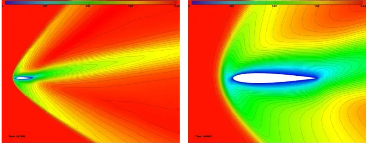
The first test case is the laminar transonic flow around the NACA0012 airfoil. For this case, the free-stream Mach number is 0.8, the angle of attack is 10 and the Reynolds number is 73. This problem has been investigated by several authors for the GAMM Workshop (see [16]) on the Solution of Compressible Navier-Stokes flows. The Mach number contours of the computed solution are depicted in Figure2, where a thick boundary layer along the airfoil surface is observed, and locally supersonic flow is attained only in a small pocket outside the edge of the viscous layer on the upper surface.
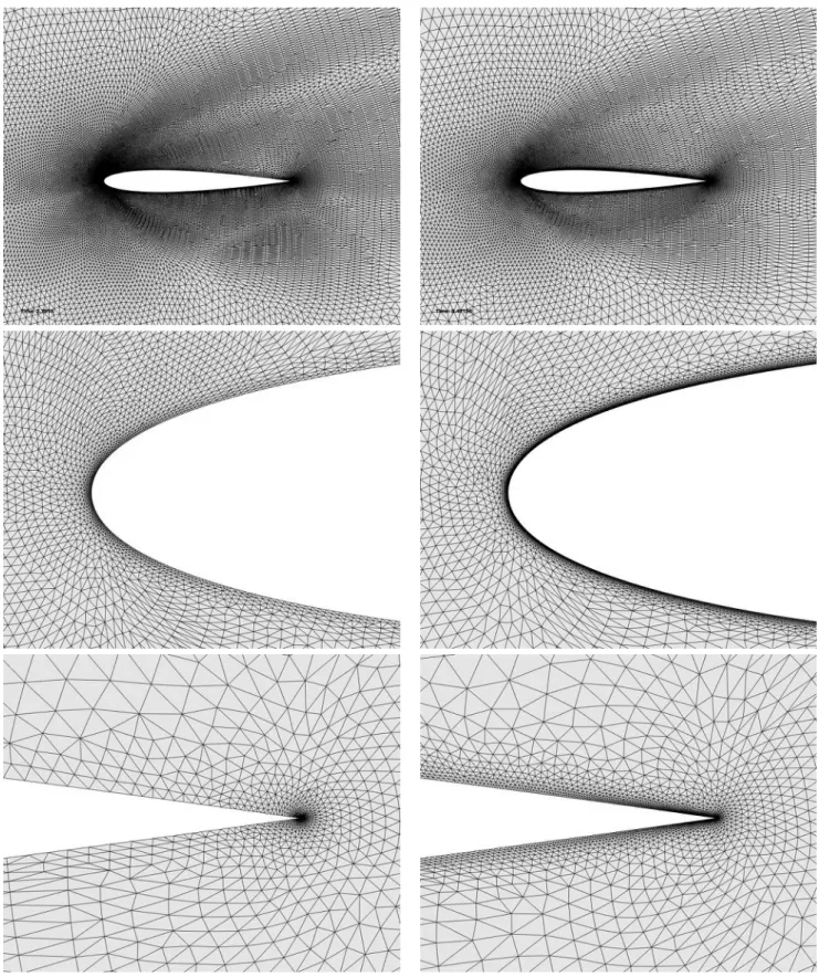
The considered functional of interest is the total drag coefficient integrated along the airfoil profile. We have considered our new a priori error estimate to compute the associated optimal anisotropic adapted meshes for varying mesh complexity. Multiple views of the resulting adapted mesh composed of about 38 000 vertices obtained after performing 6 fixed-point iterations are shown in Figure4 (right column). We observe that most of the refinement is located around the airfoil (boundary layer) and outside the edge of the viscous layer on the upper and lower regions of the domain. We also notice strong refinement at the trailing edge of the airfoil.
We also compared adapted meshes obtained using the error estimate with and without the viscous terms. In Figure 4, we compare the goal-oriented adapted mesh obtained by adapting only for the convective flux with the goal-oriented adapted mesh where both fluxes (convective and di↵usive) are considered. Both meshes have a similar number of vertices. In the far field, we observe similar anisotropic refinement, whereas close to the body we notice that the viscous error estimate adds a notable supplement of resolution in the boundary layer close to the wall and imposes a finer resolution in the vicinity of the trailing edge. As expected, the viscous terms of the error estimate govern the mesh density in the boundary layer. These di↵erences strongly impact the drag estimation as confirmed by the convergence curves of the drag presented in Figure3. We observe that our new adaptive method converges quicker to the reference drag value. For instance, the adapted mesh obtained with the viscous error estimate composed of 18 943 vertices achieves a drag value close to the adapted mesh obtained with the inviscid error estimate composed of 141 135 vertices. In other words, seven times less vertices are needed to achieve the same accuracy.
The accuracy of the computed drag values and the numerical convergence order are plotted in Figure3(right) and listed in Table1. To compute the convergence order, we have chosen as reference drag the drag obtained on the finest adapted mesh (149 465 vertices) obtained with the viscous goal-oriented error estimate: CRe fD = 0.6648091. We notice a higher order of convergence with the viscous goal-oriented error estimates (⇡ 2.25) than with the inviscid goal-oriented error estimate (⇡ 1.75). The observed convergence order of the total drag is a reasonable value for this problem.
8.2. Laminar supersonic flow around NACA0012: M = 2, ↵ = 10 and Re = 106
We present a supersonic laminar viscous flow around the same NACA0012 airfoil starting from the same initial mesh as before. The free-stream Mach number considered here is 2, with an angle of attack of 10 degrees and a laminar Reynolds number of 106. A thick bow shock appears upstream of the airfoil profile as shown in Figure5where the Mach field is pictured. The close-up view of the airfoil shows a thick boundary layer and a thick wake for this low Reynolds number flow.
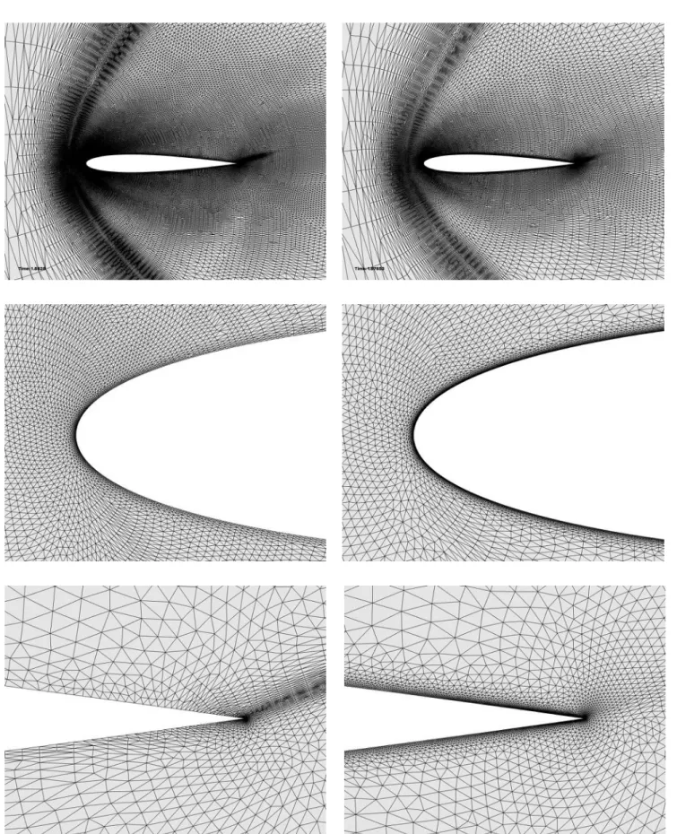
In order to perform the convergence study, several adapted meshes with di↵erent complexity have been obtained for the inviscid (no viscous terms) and the viscous goal-oriented error estimates targeting the total drag as output. Multiple views for the adapted meshes containing about 38 000 vertices are shown in Figure7for both approaches. These adapted meshes are obtained after 6 iterations of the mesh adaptation loop. We observe again that the viscous error estimate increases the mesh resolution
in the boundary layer close to the airfoil and at the trailing edge, while the inviscid one add more resolution in the bow shock vicinity.
As the targeted output functional is the drag, meshes obtained with the new error estimates are closer to our expectation. This is confirmed by the drag and error convergence curves, see Figure6and Table2. In this example too, an earlier convergence to the reference value is achieved with the new error estimate. For instance, the adapted mesh obtained with the viscous error estimate composed of 19 103 vertices achieves a similar drag value as the adapted mesh obtained with the inviscid error estimate composed of 140 924 vertices. In other words, seven times less vertices are needed to achieve the same accuracy. To analyze the convergence order, we consider as reference drag, the drag obtained on the finest mesh (149 514 vertices) with the viscous goal-oriented mesh adaptation: CRe fD =0.5549227. Then, we observe a convergence order around 2.4 for the viscous approach and 1.8 for the inviscid one. This confirms the superiority of the viscous goal-oriented error estimates and the large influence of the viscous terms in the error estimates. It also reflects the optimality of the obtained meshes.
8.3. Laminar subsonic flow around NACA0012: M = 0.5, ↵ = 3 and Re = 5 000
We present a subsonic laminar viscous flow at a higher Reynolds number around the same NACA0012 airfoil still starting from the same initial mesh. The free-stream Mach number considered here is 0.5, with an angle of attack of 3 degrees and a Reynolds number of 5 000. This test case have been initially proposed by Swanson and Turkel [51] without any angle of attack to evaluate compressible flow solver. This particular case was chosen because it has a small amount of trailing edge separation and was a good test case to check the levels of dissipation being produced by the numerical scheme. Then, this test case has been generalized to several angles of attack. These test cases require a robust flow solver to converge the solution to machine zero. Indeed, it has been shown that a non robust numerical resolution leads to unsteady solutions due to a lack of numerical convergence. This problem has been deeply investigated by Swanson et al. [50] where the authors pointed out some possible reason for failing to obtain steady solutions. They mentioned the case presented by Taube et al. in [32] where the angle of attack ↵ = 2 . The authors included adaptation in their calculation, but on a rather coarse mesh where the adaptive criterion pointed out the wake as the refinement region, resulting thus in an insufficient resolution in the vicinity of the separation point, which, as pointed out by Swanson et al., might led to unsteadiness. However, the studies conducted in [50] and on adapted meshes in [53] showed that this test case is indeed a steady problem.
The Mach contour solution is shown in Figure8. The flow separates before mid-chord location on the upper surface of the airfoil. From the streamline patterns, we can observe primary and secondary recirculating regions, with the secondary region attached to the trailing edge.
As it has been pointed out in [50] the computed aerodynamic values variation should vanish with mesh refinement. We consider the total drag coefficient Ctot
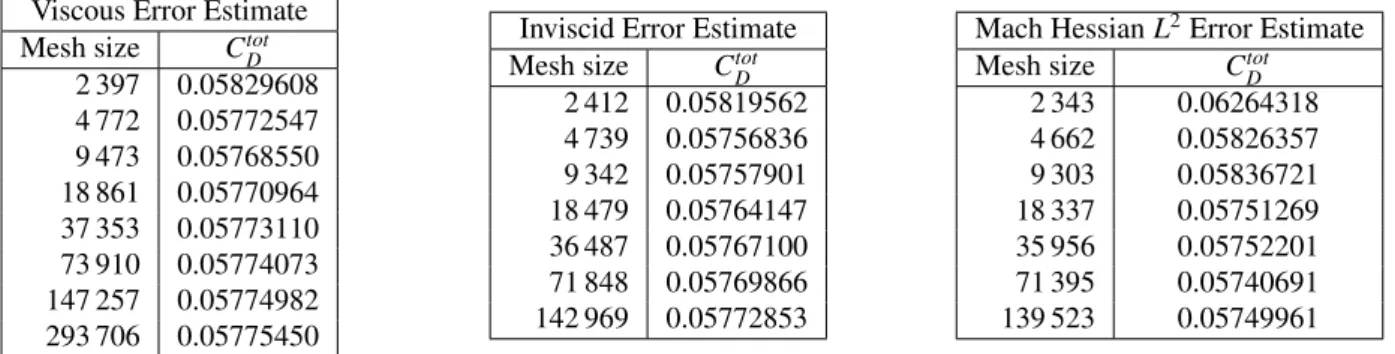
D integrated over the airfoil profile as our quantity of interest and we perform convergence studies with three di↵erent error estimates: the classical Hessian-based error estimates controlling the L2-norm of the interpo-lation error of the local Mach number field [2,40], the inviscid goal-oriented error estimate and the viscous error estimate. For each estimate, we perform multiple adaptations at di↵erent mesh complexity (from 2 000 to 140 000). For each complexity, the final adapted mesh is obtained after 6 adaptive iterations.
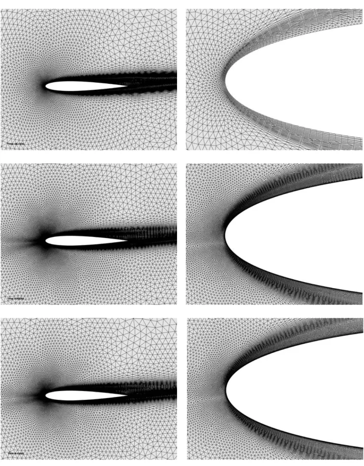
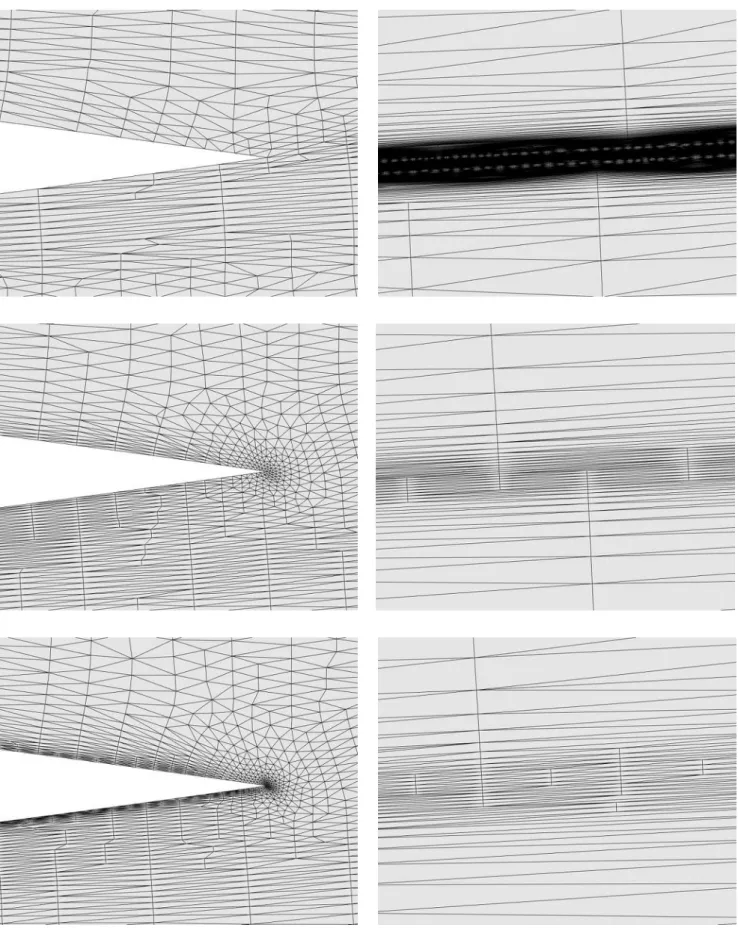
The resulting adapted meshes composed of about 38 000 vertices are shown in Figures10and11. The top pictures represent the adapted mesh obtained with the Hessian-based error estimate. We observe that the remeshing e↵ort is very poor at the leading edge, at the trailing edge, and around the airfoil profile in the boundary layer, which is what expected from this method based on minimizing the Mach errors values and not directly on improving the total drag. We can also observe that with this method the wake is highly refined (see the second column of Figure11). The middle pictures show the adapted mesh obtained with the inviscid goal-oriented error estimate. We observe that the leading edge, trailing edge and the boundary layer are more refined than using the Hessian-based error estimate while the wake has been adapted slightly. However, a closer look near the body shows that the boundary layer is not highly refine as this estimate does not take into account viscous e↵ects. The bottom pictures illustrate the adapted mesh obtained with the viscous goal-oriented error estimate. We notice that the leading edge, trailing edge and the boundary layer are even more refined and again less e↵ort has been put in the wake. A closer look near the body points out the increase refinement in the boundary layer region.
The conclusions regarding the comparison between the three adaptive methods are reinforced by Figure9and Table3where the total drag value convergence with increasing mesh size is given. We can see that the Mach-adapted method shows only a late convergence for meshes above 70 000 vertices. Both goal-oriented methods shows earlier convergence and again the viscous estimates proves to be superior to the other methods.
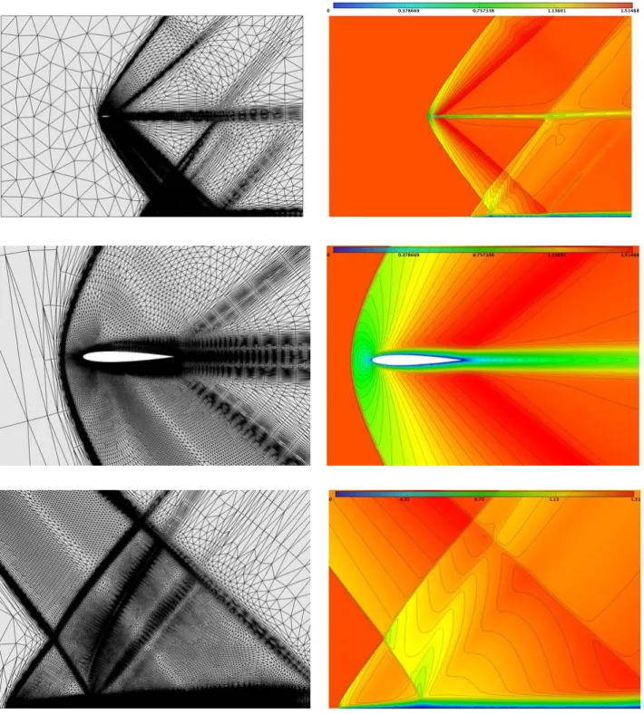
8.4. NACA0012 shock-boundary layer interaction M = 1.4, ↵ = 0 and Re = 1 000
The next example is a shock-boundary layer interaction problem in a rectangular domain of size [ 10, 20]⇥[ 10, 10] contain-ing a NACA0012 airfoil. The left, right and top parts of the domain are considered as inflow and outflow boundary conditions. The bottom part of the domain is the ground. It is considered as a slip surface except a region between x = 4 and x = 20 which
Figure 2: NACA0012 at M = 0.8, ↵ = 10 and Re = 73: Local Mach number solution field and iso-contours for the transonic laminar viscous flow obtained with the goal-oriented viscous adapted mesh composed of 37 838 vertices.
0.635 0.64 0.645 0.65 0.655 0.66 0.665 0.67 1000 10000 100000 1e+06 Cd Number of Vertices NACA0012 - M=0.8 - ALPHA=10 - Re=73
Adap GO Euler Adap GO N.-S. 1e-05 0.0001 0.001 0.01 0.1 0.001 0.01 0.1 Error Cd h=√NbrVer NACA0012 - M=0.8 - ALPHA=10 - Re=73
Adap GO Euler Adap GO N.-S.
Figure 3: NACA0012 at M = 0.8, ↵ = 10 and Re = 73: Convergence of the total drag with respect to the number of vertices (left) and error convergence (right) for the transonic laminar viscous flow computed with the inviscid (red curves) and the viscous (blue curves) goal-oriented anisotropic mesh adaptation.
Viscous Error Estimate Mesh size Ctot
D Error Conv. order
2 384 0.6564739 8.3352 ⇥ 10 3 -4 8-40 0.6610405 3.7686 ⇥ 10 3 2.24 9 562 0.6630579 1.7512 ⇥ 10 3 2.25 18 943 0.6639960 8.1310 ⇥ 10 4 2.24 37 838 0.6644963 3.1280 ⇥ 10 4 2.76 75 241 0.6647139 9.5200 ⇥ 10 5 3.46 149 465 0.6648091 Reference
-Inviscid Error Estimate Mesh size Ctot
D Error Conv. order
2 330 0.6394387 2.5370 ⇥ 10 2 -4 631 0.6511749 1.3634 ⇥ 10 2 1.81 9 139 0.6576796 7.1295 ⇥ 10 3 1.91 17 987 0.6608486 3.9605 ⇥ 10 3 1.74 35 881 0.6625947 2.2144 ⇥ 10 3 1.68 71 038 0.6635034 1.3057 ⇥ 10 3 1.55 141 135 0.6640958 7.1330 ⇥ 10 4 1.76
Table 1: NACA0012 at M = 0.8, ↵ = 10 and Re = 73: Total drag coefficient convergence, error convergence and convergence order for the viscous and inviscid error estimates.
Figure 4: NACA0012 at M = 0.8, ↵ = 10 and Re = 73: Comparison of adapted meshes composed of about 38 000 vertices for the transonic laminar viscous flow. Left, goal-oriented adapted meshwithout viscous flux contribution to optimal metric (only the Euler fluxes criterion). Right, goal-oriented adapted mesh with viscous flux contribution to optimal metric.
Figure 5: NACA0012 at M = 2, ↵ = 10 and Re = 106: Local Mach number solution field and iso-contours for the supersonic laminar viscous flow obtained with the goal-oriented viscous adapted mesh composed of 37 842 vertices.
0.52 0.525 0.53 0.535 0.54 0.545 0.55 0.555 0.56 1000 10000 100000 1e+06 Cd Number of Vertices NACA0012 - M=2 - ALPHA=10 - Re=106
Adap GO Euler Adap GO N.-S. 1e-05 0.0001 0.001 0.01 0.1 0.001 0.01 0.1 Error Cd h=√NbrVer NACA0012 - M=2 - ALPHA=10 - Re=106
Adap GO Euler Adap GO N.-S.
Figure 6: NACA0012 at M = 2, ↵ = 10 and Re = 106: Convergence of the total drag with respect to the number of vertices (left) and error convergence (right) for the transonic laminar viscous flow computed with the inviscid (red curves) and the viscous (blue curves) goal-oriented anisotropic mesh adaptation.
Viscous Error Estimate Mesh size Ctot
D Error Conv. order
2 412 0.5470249 7.8978 ⇥ 10 3 -4 800 0.5514723 3.4504 ⇥ 10 3 2.41 9 605 0.5534449 1.4778 ⇥ 10 3 2.44 19 103 0.5542634 6.5930 ⇥ 10 4 2.35 37 842 0.5546471 2.7560 ⇥ 10 4 2.55 75 590 0.5548341 8.8600 ⇥ 10 5 3.28 149 514 0.5549227 Reference
-Inviscid Error Estimate Mesh size Ctot
D Error Conv. order
2 368 0.5247889 3.0134 ⇥ 10 2 -4 602 0.5416947 1.3228 ⇥ 10 2 2.48 8 983 0.5484987 6.4240 ⇥ 10 3 2.16 17 853 0.5511675 3.7552 ⇥ 10 3 1.56 35 432 0.5529389 1.9838 ⇥ 10 3 1.86 70 159 0.5538562 1.0665 ⇥ 10 3 1.82 140 924 0.5542778 6.4490 ⇥ 10 4 1.44
Table 2: NACA0012 at M = 2, ↵ = 10 and Re = 106: Total drag coefficient convergence, error convergence and convergence order for the viscous and inviscid error estimates.
Figure 7: NACA0012 at M = 2, ↵ = 10 and Re = 106: Comparison of adapted meshes composed of about 38 000 vertices for the supersonic laminar viscous flow. Left, goal-oriented adapted meshwithout viscous flux contribution to optimal metric (only the Euler fluxes criterion). Right, goal-oriented adapted mesh with viscous flux contribution to optimal metric.
Figure 8: NACA0012 at M = 0.5, ↵ = 3 and Re = 5 000: Local Mach number solution field and iso-contours obtained on the goal-oriented viscous adapted mesh composed of 37 353 vertices.
0.057 0.058 0.059 0.06 0.061 0.062 0.063 1000 10000 100000 1e+06 Cd Number of Vertices NACA0012 - M=0.5 - ALPHA=3 - Re=5000
Adap L2 Mach Adap GO Euler Adap GO N.-S. 0.057 0.0572 0.0574 0.0576 0.0578 0.058 0.0582 0.0584 0.0586 0.0588 0.059 1000 10000 100000 1e+06 Cd Number of Vertices NACA0012 - M=0.5 - ALPHA=3 - Re=5000
Adap L2 Mach Adap GO Euler Adap GO N.-S.
Figure 9: NACA0012 at M = 0.5, ↵ = 3 and Re = 5 000: Convergence of the total drag with respect to the number of vertices for the subsonic laminar viscous flow computed with Mach Hessian-based error estimate (pink curve), the inviscid (red curves) and the viscous (blue curves) goal-oriented error estimates.
Viscous Error Estimate Mesh size Ctot
D 2 397 0.05829608 4 772 0.05772547 9 473 0.05768550 18 861 0.05770964 37 353 0.05773110 73 910 0.05774073 147 257 0.05774982 293 706 0.05775450
Inviscid Error Estimate Mesh size Ctot
D 2 412 0.05819562 4 739 0.05756836 9 342 0.05757901 18 479 0.05764147 36 487 0.05767100 71 848 0.05769866 142 969 0.05772853
Mach Hessian L2Error Estimate Mesh size Ctot
D 2 343 0.06264318 4 662 0.05826357 9 303 0.05836721 18 337 0.05751269 35 956 0.05752201 71 395 0.05740691 139 523 0.05749961
Table 3: NACA0012 at M = 0.5, ↵ = 3 and Re = 5 000: Total drag coefficient convergence for the viscous, the inviscid, and the Hessian-based error estimates.
is a no-slip surface where develops a boundary layer. The leading edge of the airfoil is located at (0, 0); this represents a distance of 10 chords length from the ground. The airfoil is also considered as a slip surface.
As the supersonic flow conditions are a free-stream Mach number of 1.4, an angle of attack of 0 and a Reynolds number of 1 000; the flow is strongly shock dominated. It is then interesting to investigate the interaction between the bow shock emitted
Figure 10: NACA0012 at M = 0.5, ↵ = 3 and Re = 5 000: Comparison of adapted meshes composed of about 38, 000 vertices for the subsonic laminar viscous flow. Top, Hessian-based error estimates controlling the L2-norm of the interpolation error of the local Mach number field. Middle, goal-oriented adapted mesh without viscous flux contribution to optimal metric (only the Euler fluxes criterion). Right, goal-oriented adapted mesh with viscous flux contribution to optimal metric.
Figure 11: NACA0012 at M = 0.5, ↵ = 3 and Re = 5 000: Comparison of adapted meshes composed of about 38, 000 vertices for the subsonic laminar viscous flow. Top, Hessian-based error estimates controlling the L2-norm of the interpolation error of the local Mach number field. Middle, goal-oriented adapted mesh without viscous flux contribution to optimal metric (only the Euler fluxes criterion). Right, goal-oriented adapted mesh with viscous flux contribution to optimal metric.