HAL Id: cea-01179958
https://hal-cea.archives-ouvertes.fr/cea-01179958
Submitted on 23 Jul 2015
HAL is a multi-disciplinary open access
archive for the deposit and dissemination of
sci-entific research documents, whether they are
pub-lished or not. The documents may come from
teaching and research institutions in France or
abroad, or from public or private research centers.
L’archive ouverte pluridisciplinaire HAL, est
destinée au dépôt et à la diffusion de documents
scientifiques de niveau recherche, publiés ou non,
émanant des établissements d’enseignement et de
recherche français ou étrangers, des laboratoires
publics ou privés.
Dynamic identification of robots with a dry friction
model depending on load and velocity
P. Hamon, M. Gautier, Philippe Garrec
To cite this version:
P. Hamon, M. Gautier, Philippe Garrec. Dynamic identification of robots with a dry friction model
depending on load and velocity. IEEE/RSJ 2010 International Conference on Intelligent Robots and
Systems IROS 2010, Oct 2010, tawain, France. pp.6187-6193, �10.1109/IROS.2010.5649189�.
�cea-01179958�
Abstract—Usually, the joint transmission friction model for
robots is composed of a viscous friction force and of a constant dry sliding friction force. However, according to the Coulomb law, the dry friction force depends linearly on the load driven by the transmission. It follows that this effect must be taken into account for robots working with large variation of the payload or inertial and gravity forces, and actuated with transmissions as speed reducer, screw-nut or worm gear. This paper proposes a new inverse dynamic identification model for n degrees of freedom (dof) serial robot, where the dry sliding friction force is a linear function of both the dynamic and the external forces, with a velocity-dependent coefficient. A new identification procedure groups all the joint data collected while the robot is tracking planned trajectories with different payloads to get a global least squares estimation of inertial and new friction parameters. An experimental validation is carried out with a joint of an industrial robot.
I. INTRODUCTION
HE usual identification method is based on the inverse dynamic model (IDM) which is linear in relation to the dynamic parameters, and uses least squares (LS) technique. This procedure has been successfully applied to identify inertial and friction parameters of a lot of prototypes and industrial robots [1]- [10]. An approximation of the kinematic Coulomb friction, F sign qC ( )ɺ , is widely used to model friction force at non zero velocity qɺ , assuming that the friction force FC is a constant parameter. It is identified by
moving the robot without any load (or external force) or with constant given payloads [9].
However, the Coulomb law suggests that FC depends on
the transmission force driven in the mechanism. It depends on the dynamic and on the external forces applied through the joint drive chain. Consequently for robots with varying load, the identified IDIM is no more accurate when the transmission uses industrial speed reducer, screw-nut or worm gear because their efficiency significantly varies with the transmitted force. The significant dependence on load has been often observed for transmission elements [15]- [19] through direct measurement procedures. Moreover, the mechanism efficiency depends on the sense of power transfer leading to two distinct sets of friction parameters. In addition, when the robot moves at very low velocity, as for teleoperation, one observes a velocity-dependency of the dry
friction.
This paper presents a new inverse dynamic identification model for n degrees of freedom (dof) serial robot, where the dry sliding friction force FC is a linear function of both the dynamic and the external forces, with asymmetrical behavior depending on the signs of joint force and velocity, and a variation depending on the velocity amplitude. A new identification procedure is proposed. All the joint position and joint force data collected in several experiments, while the robot is tracking planned trajectories with different payloads, are concatenated to calculate a global least squares estimation of both the inertial and the new friction parameters.
An experimental validation is carried out on the third joint of an industrial robot: Stäubli RX130L [25]. Both models are compared.
II. USUAL INVERSE DYNAMIC MODELING AND IDENTIFICATION
A. Modeling
In the following, all mechanical variables are given in SI units in the joint space. All forces, positions, velocities and accelerations have a conventional positive sign in the same direction. That defines a motor convention for the mechanical behavior.
The dynamic model of a rigid robot composed of n moving links is written as follows [11]:
dyn = in+ f + ext
τ τ τ τ (1)
where:
• τdyn is the (nx1) vector of dynamic forces due to the
inertial, centrifugal, Coriolis, and gravitational effects:
( ) ( ) ( )
dyn = ɺɺ+ ,ɺ ɺ+
τ M q q C q q q Q q (2)
where q, ɺq and ɺɺq are respectively the (nx1) vectors of
generalized joint positions, velocities and accelerations,
M(q) is the (nxn) robot inertia matrix, C q q is the (nxn) ( , )ɺ matrix of centrifugal and Coriolis effects, Q(q) is the (nx1) vector of gravitational forces.
• τin is the (nx1) input torque vector on the motor side of the drive chain:
Dynamic Identification of Robots with a Dry Friction Model
Depending on Load and Velocity
P. Hamon
(1), M. Gautier
(2), and P. Garrec
(1)(1)
CEA, LIST, Interactive Robotics Laboratory, 18 route du Panorama, BP6, Fontenay-aux-Roses, F-92265, France.
(2)
University of Nantes/IRCCyN, 1 rue de la Noë, BP 92101, Nantes Cedex 03, F-44321, France.
T
Intelligent Robots and Systems October 18-22, 2010, Taipei, Taiwan
( 0)
in = f f − f
τ g v v (3)
where v is the (nx1) vector of current references of the f current amplifiers, vf0 is a (nx1) vector of amplifiers offsets, gf is the (nxn) matrix of the drive gains,
f = i t
g NG K (4)
N is the (nxn) gear ratios matrix of the joint drive chains
(qɺm =Nqɺ with qɺm the (nx1) velocities vector on the motor
side), Gi is the (nxn) static gains diagonal matrix of the
current amplifiers, Kt is the (nxn) diagonal matrix of the
electromagnetic motor torque constants [14].
• τf is the (nx1) vector of the loss force due to frictions.
Usually, it is approximated with a viscous friction and a dry friction:
( ) f = − Vɺ− C ɺ − Coff
τ F q F sign q F (5)
where FV is the (nxn) diagonal matrix of viscous
parameters, FC is the (nxn) diagonal matrix of dry friction
parameters, and sign(.) denotes the sign function, FCoff is a
(nx1) vector of asymmetrical Coulomb friction force between positive and negative velocities. This friction model is linear to FV and FC (Fig. 1.a).
• τext is the (nx1) external forces vector in the joint space. Thus (1) becomes:
( ) ( )
( )
0
dyn ext f f V C Coff f f
out V C off − = − − − + ⇔ = − − − ɺ ɺ ɺ ɺ τ τ g v F q F sign q F g v τ τ F q F sign q τ (6)
where τout =τdyn−τext is the output force (the load force) of the drive chain, τoff =FCoff +g vf f0 is an offset force that
regroups the amplifier offset and the asymmetrical Coulomb friction coefficient.
f f =
τ g v (7)
is the motor force, without offset, and defined by vf which is
the current reference calculated by the numerical control and stored for the identification.
Then (1) can be rewritten as the inverse dynamic model (IDM) which calculates the motor torque vector τ as a function of the generalized coordinates:
( ) ( ) ( ) ( ) ( ) C V off ext out C V off , = + + + + + − = + + + ɺɺ ɺ ɺ ɺ ɺ ɺ ɺ τ M q q C q q q Q q F sign q F q τ τ τ F sign q F q τ (8) B. Identification
The choice of the modified Denavit and Hartenberg frames attached to each link allows to obtain a dynamic model linear in relation to a set of standard dynamic parameters χSt [6], [11]:
( )
St , , St
= ɺ ɺɺ
τ D q q q χ (9)
where DSt(q q q, ,ɺ ɺɺ) is the regressor and χSt is the vector of the standard parameters which are the coefficients XXj, XYj,
XZj, YYj, YZj, ZZj of the inertia tensor of link j denoted j
Jj, the mass of the link j called mj, the first moments vector of link j
around the origin of frame j denoted jMj = [MXj MYj MZj]
T
, the friction coefficients FVj, FCj, the actuator inertia called
Iaj, and the offset τoff j. The velocities and accelerations are
calculated using well tuned band pass filtering of the joint position [7].
The base parameters are the minimum number of parameters from which the dynamic model can be calculated. They are obtained by eliminating and by regrouping some standard inertial parameters [12], [13]. The minimal inverse dynamic model can be written as:
( , , ) = ɺ ɺɺ
τ D q q q χ (10)
where D q q q( , ,ɺ ɺɺ) is the minimal regressor and χ is the vector of the base parameters.
The inverse dynamic model (10) is sampled while the robot is tracking a trajectory to get an over-determined linear system such that [6]:
( )= ( , ,ɺ ɺɺ) +
Y τ W q q q χ ρ (11)
with Y(τ) the measurements vector, W the observation matrix and ρ the vector of errors.
The LS solution ˆχ minimizes the 2-norm of the vector of errors ρ. W is a (r×b) full rank and well conditioned matrix where r=N x ne , with Ne the number of samples on the
trajectories. The LS solution ˆχis given by:
(
)
1T T
ˆ = − = +
χ W W W Y W Y (12)
It is calculated using the QR factorization of W. Standard deviations
i ˆ
χ
σ are estimated using classical and simple results from statistics. The matrix W is supposed to be deterministic, and ρ, a zero-mean additive independent noise, with a standard deviation such as:
(
T)
E 2
r
ρρ = =σρ
C ρρ I (13)
where E is the expectation operator and Ir, the (r×r) identity
matrix. An unbiased estimation of σρ is:
( )
2
2 ˆ
ˆρ r b
σ = Y−Wχ − (14)
The covariance matrix of the standard deviation is calculated as follows: T 2 T 1 χχ E ( )( ) σρ( ) ˆ ˆ ˆ ˆ − = − − = C χ χ χ χ W W (15) i 2 ˆ Cˆ ˆ ii χ χχ
σ = is the ith diagonal coefficient of Cχχˆ ˆ. The
relative standard deviation ri ˆ %σχ is given by: ri i ˆ ˆ ˆi %σχ =100σχ χ (16)
However, experimental data are corrupted by noise and error modeling and W is not deterministic. This problem can be solved by filtering the measurement vector Y and the columns of the observation matrix W as described in [7], [8].
III. NEW DRY FRICTION MODEL AND IDENTIFICATION In this section, we introduce a dry friction model dependent on the load, that is τout, and on the velocity ɺq .
A. Load-Dependent Friction Model
The Coulomb friction is still written FCsign( )q , with FCɺ a (nxn) diagonal matrix. But here, for each link j, FC j , j( ) (the (j,j)th element of the matrix F ) depends linearly on the C
absolute value of the load of joint j which is τout j (Fig. 1.b), [15]- [19]. As one can see in II.B, τout j is a function of
, , ɺ ɺɺ
q q q and is linear in relation to base parameters.
Then the inverse dynamic model for each link j becomes:
(
)
( ) ( )j out j j out j j sign qj V j , jqj off j
τ =τ + α τ +β ɺ +F ɺ +τ (17)
where αj and βj are parameters to be identified. These new parameters depend on the mechanical structure of the reducers used to actuate the robot.
For ease of understanding, the subscript j is omitted for all variables in the following to simplify the notation.
Fig. 1. a) Usual friction model with constant dry friction + viscous friction. b) Model with load-dependent dry friction + viscous friction.
c) Model with load- and velocity-dependent dry friction + viscous friction.
The inverse dynamic model can be written as follows:
( ) ( )
out out sign q sign q F qV off
τ =τ +α τ ɺ +β ɺ + ɺ+τ (18)
And with τout =τoutsign(τout) and ( out) ( ) ( out ) ( out)
signτ sign qɺ =sign τ qɺ =sign P , one obtains:
( ) ( )
out outsign Pout sign q F qV off
τ =τ +ατ +β ɺ + ɺ+τ (19)
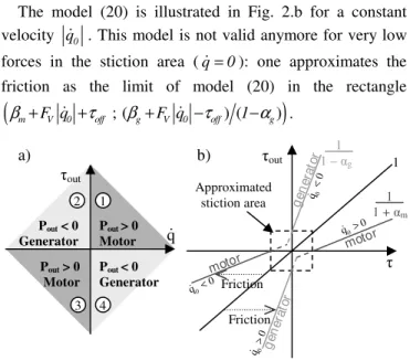
Thus, the IDM depends on the signs of the output power out out
P =τ qɺ. One defines 4 quadrants in the frame (q,ɺτout), which can be grouped two by two (Fig. 2.a). In the quadrants 1 and 3, Pout is positive and the actuator has a motor
behavior. In the quadrants 2 and 4, Pout is negative and the actuator has a generator behavior which may save the power to the power supply, assuming a 4 quadrants amplifier.
B. Dry Friction Model Depending on the Power Sign In the model (19), α and β do not depend on the output power sign. But, generally they take different values: αm and βm for the motor quadrants, and αg and βg for the generator quadrants.
( ) ( )
( ) ( )
out m out m V off
out g out g V off
P 0 1 sign q F q P 0 1 sign q F q τ α τ β τ τ α τ β τ > ⇒ = + + + + < ⇒ = − + + + ɺ ɺ ɺ ɺ (20)
The model (20) is illustrated in Fig. 2.b for a constant velocity qɺ0 . This model is not valid anymore for very low forces in the stiction area ( qɺ=0): one approximates the friction as the limit of model (20) in the rectangle
(
βm+F qV ɺ0+τoff ; (βg+F qV ɺ0 −τoff) (1−αg))
.Fig. 2. a) Four quadrants frame (q,ɺτout) for motor or generator behavior. b) Asymmetrical friction for a given velocity qɺ and the stiction area. 0
C. Dry Friction Model Depending on the Velocity For a robot moving at low velocities, one observes a dry friction variation, functions of the velocity, which is similar to the Stribeck model (Fig. 1.c), [20], [21], [22].
if and ( ) if and ( ) if out st out st out out st q 0 F F F sign q 0 F F q q 0 τ τ τ τ = < = = ≥ ≠ ɺ ɺ ɺ ɺ (21) with:
(
)
( ) ( ) q / qs ( ) sl st sl F qɺ = F + F −F e−ɺ ɺ sign qɺ (22) where qɺS is a velocity constant, Fst is the dry friction in stiction and Fsl is the dry friction in sliding mode.To combine the variation due to the load (17) with the one due to velocity (22), one takes:
et sl out st out F =α τ +β F =γ τ +δ (23) Then, (22) becomes: a) b) qɺ Pout > 0 Motor Pout > 0 Motor Pout < 0 Generator τout Pout < 0 Generator 1 4 3 2 τout τ 1 Approximated stiction area Friction Friction 1 + αm 1 1 – αg 1 motor gen erat or motor gen erat or 0 qɺ0< 0 q0 < ɺ 0 q0 > ɺ 0 q0> ɺ b) qɺ β -β out τ increases a) qɺ Fc -Fc f Coff (τ F ) − + c) qɺ out τ increases f Coff (τ F ) − + −(τf+FCoff)
(
)
(
)
(
)
( ) ( ) ( ) ( ) ( ) ( ) ( ) S S S q qout out out
q q q q out out F q e sign q e sign P e sign q α τ β γ τ δ α τ β α γ α τ β δ β − − − = + + + − − = + − + + − ɺ ɺ ɺ ɺ ɺ ɺ ɺ ɺ ɺ (24)
Because of the dependence on power sign, one has 2 sets of parameters α , β , γ , δ for the 2 behaviors: motor and generator. Considering am = +1 αm, bm =γm−αm, cm =βm,
m m m
d =δ −β , and ag = −1 αg, bg =γg −αg, cg =βg,
g g g
d =δ −β , the inverse dynamic model becomes:
( ) ( ) ( ) ( ) S S S S out q q q q
m out m out m m V off
out
q q q q
g out g out g g V off
P 0 a b e c sign q d e sign q F q P 0 a b e c sign q d e sign q F q τ τ τ τ τ τ τ τ − − − − > ⇒ = + + + + + < ⇒ = − + + + + ɺ ɺ ɺ ɺ ɺ ɺ ɺ ɺ i ɺ ɺ ɺ i ɺ ɺ ɺ (25)
D. Friction Identification Method
In order to keep a IDM linear in relation to the parameters, one decides on an a priori value of qɺ . This constant S represents the exponential transitional behavior between stiction and sliding, that is about 3∗ ɺ , more or less 5%. qS Measurements show that the amplitude of this transitional behavior is close to 10% of the nominal velocity 1.2 rad/s, that is qɺS =0.04 rad/s. A final adjustment to qɺS =0.03 rad/s at the moment of the identification gives a minimal residual
ρ a little lower. This value for qɺ is close to the value S given in [22] for a Kuka IR 161 robot.
Furthermore, the model (25) depends on the sign of Pout which is unknown. To overcome this problem, the samples of τ measurements are selected outside of the stiction area ( qɺ=0 – Fig. 2.b) in order to get the same sign for τout and τ. This allows to get the sign of Pout with:
( out) ( out ) ( ) ( )
sign P =signτ qɺ =signτqɺ =sign P (26) One can then write the IDM linear in relation to parameters and use the LS technique. To have only one expression instead of two in (25), 3 variables are introduced,
P+, P−, and Exp, defined by:
( ) 1 sign P P 2 + = + , 0 1 P> ⇔P+ = , P<0 ⇔P+ = (27) 0 ( ) 1 sign P P P 2 − = − = + (28) S q q xp E =e−ɺ ɺ (29)
The inverse dynamic model is then written:
( ) ( ) ( ) ( ) ( ) ( ) m m xp out g g xp out m m xp g g xp V off P a b E P a b E ... ... P c d E sign q P c d E sign q F q τ τ τ τ + − + − = + + − + + ɺ + + ɺ + ɺ+ (30)
As τout is linear in relation to parameters, so is τ .
IV. EXPERIMENTAL SETUP AND IDENTIFICATION
A. Study case: Stäubli RX130L Robot
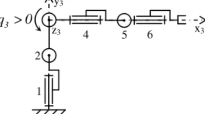
The Stäubli RX130L robot is an industrial robot with 6 rotational joints. The joint 3 has been chosen for this study because unlike the joint 1, it has large gravity variation, and no compensation gravity spring contrary to the joint 2. The links 1 and 2 are lined up and locked in a vertical position. The arm 3 is composed of the links 4, 5 and 6 brought into line with the link 3 and locked (Fig. 3), with a total mass of about 30 kg and a length of 1.33 m. The maximum velocity is 1.2 rad/s and the maximum acceptable load at the extremity is 10 kg.
The inverse dynamic model of joint 3 is written:
( ) ( ) ( )
3 J q3 3 MX gcos q3 3 MY g sin q3 3 F sign qC3 3 F qV3 3 off 3
τ = ɺɺ+ + + ɺ + ɺ +τ (31)
where:
• J3 =Ia3+ZZ3 is the inertia moment Ia3 of the drive
chain plus the inertia moment ZZ3 of the arm, • g =9.81 m/s2 is the gravity acceleration.
All variables and parameters are given in SI units on the joint space. In the following, the subscript 3 is omitted to simplify the notation.
Fig. 3. RX130L drawing: joints 1, 2, 4, 5 and 6 locked in position.
B. Data Acquisition
The identification of dynamic parameters is carried out with and without payloads: two different additional masses can be fixed to the arm extremity. To excite properly the friction parameters to be identified, sinusoidal and trapezoidal velocities trajectories were used.
The estimation of qɺ and qɺɺ are carried out with pass band filtering of q consisting of a low pass Butterworth filter and a central derivative algorithm. The Matlab function filtfilt can be used [23]. The motor torque is calculated using the current reference (7). In order to cancel high frequency ripple in τ, the vector Y and the columns of the observation matrix W are both low pass filtered and decimated. This parallel filtering procedure is carried out with the Matlab decimate function [2], [10].
C. Identification
To identify the load-dependent friction, measurements
1 2 4 5 6 x3 y3 z3 3 q >0 6190
with known payloads are used. Gravity and inertial forces due to the additional mass fixed to the robot extremity have to be added in the IDM.
Let Rm be the frame set at the center of gravity Gm of the
additional masse Ma, and parallel to the frame R x , y , z3( 3 3 3) linked to the arm (Fig. 3). One gives the inertia matrix IGa of
the additional mass which is a disk with a radius r and a thickness l: ( ) ( ) ( ) m m 2 a 2 2 Ga a 2 2 a G ,R M r 2 0 0 I 0 M r 4 l 12 0 0 0 M r 4 l 12 = + + (32)
The vector of translation between R3 and Rm is T
a
T=L 0 0 and as the 2 frames are parallel, one can apply the Huygens theorem:
( ) ( ) 2 a 2 2 a a 2 2 2 a a a M r 2 0 0 J 0 M r 4 l 12 0 0 0 M r 4 l 12 M L = + + + (33)
As the terms r² and e² are negligible, compared with
2 a
L , one keeps only the term M L qa 2aɺɺ .
For the gravity, considering the vector of translation T, one has: M L g cos qa a ( ).
Thus, for the samples τ( )k with an additional mass Ma k( ), (31) becomes: ( ) ( ) ( ) ( ) ( ) ( ) ( ) 2 k a k a a k a C V off
Jq MXg cos q MYg sin q M L q ...
...M L g cos q F sign q F q τ τ = + + + + + + + ɺɺ ɺɺ ɺ ɺ (34) where:
• Ma k( ) is one of the additional masses, fixed to robot
extremity, with accurate weighed values: 0 kg, 3.4584 kg and 6.970 kg,
• La is the length from the joint 3 to the additional mass
position (measured distance): 1.277 m
At a first step, to identify the usual model with all samples, one distinguishes the weighed mass Maw and the mass Mae
estimated by the identification. Thus, the usual model is:
( ) ( ) ( ) ( ) ( ) ( ) ( ( )) ( ) k ae k aw k a a C V off aw k
Jq MXg cos q MYg sin q ... M ... M L L q g cos q F sign q F q M τ τ = + + + + + + + ɺɺ ɺɺ ɺ ɺ (35)
Then, the sampled measurements, for k from 1 to 3, are concatenated using the Maw k( ) corresponding to each experiment (k), to get the linear system:
usual = usual usual+ usual
Y W χ ρ (36)
with the measurements vector, the observation matrix, and the vector of base parameters below:
T T T T usual = = (1) (2) (3) Y τ τ τ τ (37) ( ) ( ) ( ( )) ( ) usual=ɺɺ aw a aɺɺ+ signɺ ɺ
W q gcos q gsin q M L Lq gcos q q q 1 (38)
T ae usual C V off aw M J MX MY F F M τ = χ (39)
At a second step, the proposed model is identified with:
new = new new+ new
Y W χ ρ (40)
with the measurements vector, the observation matrix, and the vector of base parameters defined as follows:
new = usual= Y Y τ (41) ( ) ( ) ( ) ( ) ( ( )) ( ( )) ( ) ( ) ( ) ( ) new xp xp xp a a a xp a a a xp xp xp a ... ... ... ... ... ... ... ... ... ... + + + + + + + + − − − − − − − = + − − − ɺɺ ɺɺ ɺɺ ɺɺ ɺɺ ɺɺ W P q P E q P gcos q
P E gcos q P gsin q P E gsin q
P M L L q gcos q P E M L L q+ gcos q P q P E q P gcos q
P E gcos q P gsin q P E gsin q
P M L ( ( )) ( ( )) ( ) ( ) ( ) ( ) a a xp a a a xp xp ... ... − + + − − + − + ɺɺ ɺɺ ɺ ɺ ɺ ɺ ɺ L q gcos q P E M L L q gcos q P sign q P E sign q P sign q P E sign q q 1
(42) T new m m m m m m m m g g g g g g g g m m g g V off a J b J a MX b MX a MY b MY a b ... ... a J b J a MX b MX a MY b MY a b ... ... c d c d F τ = χ (43)
The expressions of Wnew and χnew are obtained by inserting τout=Jq MXgcos qɺɺ+ ( )+MYgsin q( )+M L L q M gcos qa a(aɺɺ+ a ( )) in the inverse dynamic model (30).
Here P , + P , and − Exp are diagonal matrices, with:
( ) ( )i ( )i qi qS i ,i i ,i xp i ,i 1 sign 1 sign , , e 2 2 − + + − − = P = P = ɺ ɺ P P Ε (44)
The two models are compared using exactly the same identification method with the same measurements.
D. Results
The significant values identified with usual IDM and OLS regressions are given in Table I and those with the new IDM in Table II (the parameters with a large relative deviation are not significant and have been eliminated). For each model, Fig. 4 and Fig. 5 present a direct validation comparing the actual τ with its predicted value Wˆχ. Moreover, Table III
presents the relative norm of errors ρ Y for the two models and for several sets of experiments: all measurements (all velocities), with low velocities (0 to 10% of the maximum velocity) or high velocities (35% to 100% of the maximum velocity). Finally, Table IV compares the relative norms of errors for the two models, with two different identifications: the first one is carried out with all measurements, that is with variation of the payload fixed to arm extremity, and the second one is carried out with only the samples obtained without payload.
As one can see in all figures and tables, the new dynamic model improves the residual.
TABLE I
IDENTIFIED VALUES WITH USUAL IDM
Parameters Identified Values Standard deviation * 2 Relative deviation J 30.921 0.283 0.46 % MX 21.109 0.016 0.04 % Mae/Map 0.922 0.003 0.15 % FC 39.890 0.084 0.11 % FV 29.429 0.395 0.67 % τoff 9.931 0.077 0.39 % TABLE II
IDENTIFIED VALUES WITH NEW IDM
Parameters Identified Values Standard deviation * 2 Relative deviation amJ 32.420 0.262 0.40 % amMX 22.204 0.033 0.07 % bmMX 1.621 0.050 1.55 % am 0.942 0.005 0.25 % bm 0.240 0.008 1.72 % agJ 29.294 0.276 0.47 % agMX 19.432 0.042 0.11 % bgMX 1.798 0.051 1.43 % ag 0.915 0.005 0.27 % bg 0.266 0.008 1.59 % cm 21.152 0.143 0.34 % cg 15.588 0.244 0.78 % FV 48.139 0.317 0.33 % τoff 9.950 0.051 0.26 % TABLE III
RELATIVE NORM OF ERRORS WITH BOTH MODELS
Measurements used Usual model New model
All Samples (all velocities) 0.0733 0.0484 Samples with low velocities 0.0737 0.0401 Samples with high velocities 0.0863 0.0881
TABLE IV
RELATIVE NORM OF ERRORS FOR 2 IDENTIFICATIONS
Identification carried out Usual model New model
With payload variations 0.0733 0.0484
Without payload 0.0742 0.0598 0 2 4 6 8 10 12 14 x 104 -500 -400 -300 -200 -100 0 100 200 300 400 500 Samples In p u t to rq u e τ ( N .m ) Measurement Estimation Error
Fig. 4. Direct validation performed with usual IDM.
0 2 4 6 8 10 12 14 x 104 -500 -400 -300 -200 -100 0 100 200 300 400 500 Samples In p u t to rq u eτ ( N .m ) Measurement Estimation Error
Fig. 5. Direct validation performed with new IDM.
V. DISCUSSION
The parameters of the new model are identifiable (low standard deviation) and so significant. The identification process does not change as the new model is still linear in relation to the parameters. The originality is that the global identification groups all measurements, with all payloads, in only one LS process. The main difficulty is to distinguish the different behaviours, motor and generator, but a solution has been proposed along this paper. One can also note that the measurements have to be more exciting than usual: each test has to be done with different loads and low velocities to highlight the effect on the friction variations. So, this identification protocol is more time-consuming and the setting up must be adapted for the measurements with additional masses.
The figures of direct validation show an improvement of the estimated torque by the new model, which is confirmed by the Table III. Indeed, one observes a decrease of 34% in the relative norm of errors. The improvement is mostly important for the low velocities where the errors are divided 6192
by two, thanks to the new model (decrease of 46%). At high velocity, the friction term with the exponential function approaches zero, and the new model is equivalent to the usual.
Moreover, the Table IV shows that the model is especially interesting for robots carrying some payloads. However, for a robot without payload but with high gravity variation, as the third joint of the RX130L, one obtains still a decrease of 19% of the errors.
Finally, this new model can be easily applied to a multi dof robot, using (30) for each joint j.
This model is important for example in teleoperation, where the robots work at reduced velocity and can carry payloads or perform tasks with the effector subjected to external forces.
VI. CONCLUSION
This paper has presented a new dry friction model, with load- and velocity-dependency, and its identification method. The inverse dynamic model and the identification of its parameters have been successfully validated on a rotational joint of an industrial robot. As a result, one observes a significant improvement comparing to the usual model, for joints with large load variations, and especially at low velocity. Robots carrying important masses or with large inertial or gravity variations are concerned. In addition, this technique can be applied to multi dof robots.
Future works concern the application of this model to the multi dof robot and for different types of transmission. Then, the model will be used for torques monitoring and collision detection.
ACKNOWLEDGMENT
The authors thank the AREVA society [24] for the availability of the Stäubli RX130L robot.
REFERENCES
[1] C. G. Atkeson, C. H. An, and J. M. Hollerbach, “Estimation of Inertial Parameters of Manipulator Loads and Links”, in Int. J. of
Robotics Research, vol. 5(3), 1986, pp. 101-119.
[2] J. Swevers, C. Ganseman, D. B. Tückel, J. D. de Schutter, and H. Van Brussel, “Optimal Robot excitation and Identification”, IEEE Trans.
on Robotics and Automation, vol. 13(5), 1997, pp. 730-740.
[3] P. K. Khosla and T. Kanade, “Parameter Identification of Robot Dynamics”, in Proc. 24th IEEE Conf. on Decision Control, Fort-Lauderdale, December 1985.
[4] M. Prüfer, C. Schmidt, and F. Wahl, “Identification of Robot Dynamics with Differential and Integral Models: A Comparison”, in
Proc. 1994 IEEE Int. Conf. on Robotics and Automation, San Diego,
California, USA, May 1994, pp. 340-345.
[5] B. Raucent, G. Bastin, G. Campion, J. C. Samin, and P. Y. Willems, “Identification of Barycentric Parameters of Robotic Manipulators from External Measurements”, Automatica, vol. 28(5), 1992, pp. 1011-1016.
[6] M. Gautier, “Identification of robot dynamics”, in Proc. IFAC Symp.
On Theory of Robots, Vienna, Austria, December 1986, pp. 351-356.
[7] M. Gautier, “Dynamic identification of robots with power model”, in
Proc. IEEE Int. Conf. on Robotics and Automation, Albuquerque,
1997, pp. 1922-1927.
[8] M. Gautier and P. H. Poignet, “Extended Kalman filtering and weighted least squares dynamic identification of robot”, Control
Engineering Practice, 2001.
[9] W. Khalil, M. Gautier, and P. Lemoine, “Identification of the payload inertial parameters of industrial manipulators”, IEEE Int. Conf. on
Robotics and Automation, Roma, Italia, April 2007, pp. 4943-4948.
[10] H.Kawasaki and K. Nishimura, “Terminal-link parameter estimation and trajectory control of robotic manipulators”, IEEE J. of Robotics
and Automation, vol. RA-4(5), pp. 485-490, 1988.
[11] W. Khalil and E. Dombre, Modeling, identification and control of
robots. Hermes Penton, London, 2002.
[12] M. Gautier and W. Khalil, “Direct calculation of minimum set of inertial parameters of serial robots”, IEEE Trans. on Robotics and
Automation, vol. RA-6(3), 1990, pp. 368-373.
[13] M. Gautier, “Numerical calculation of the base inertial parameters”, J.
of Robotic Systems, vol. 8(4), August 1991, pp. 485-506.
[14] P. P. Restrepo and M. Gautier, “Calibration of drive chain of robot joints”, in Proc. 4th IEEE Conf. on Control Applications, Albany, 1995, pp. 526-531.
[15] A. Gogoussis and M. Donath, “Coulomb friction effects on the dynamics of bearings and transmissions in precision robot mechanisms”, in Proc. IEEE Int. Conf. on Robotics and Automation, Philadelphia, Pennsylvania, April 1988, vol. 3, pp. 1440-1446. [16] M. E. Dohring, E. Lee, and W. S. Newman, “A load-dependent
transmission friction model: theory and experiments”, in Proc. IEEE
Int. Conf. on Robotics and Automation, Atlanta, Georgia, May 1993,
vol. 3, pp. 430-436.
[17] C. Pelchen, C. Schweiger, and M. Otter, “Modeling and simulation the efficiency of gearboxes and of planetary gearboxes”, in Proc. 2nd
International Modelica Conference, Oberpfaffenhofen, Germany,
March 2002, pp. 257-266.
[18] N. Chaillet, G. Abba, and E. Ostertag, “Double dynamic modelling and computed-torque control of a biped robot”, in Proc. IEEE/RSJ/GI Int. Conf. on Intelligent Robots and Systems, 'Advanced Robotics
Systems and the Real Word', Munich, Germany, September 1994, vol.
2, pp. 1149-1155.
[19] P. Garrec, J.-P. Friconneau, Y. Measson, and Y. Perrot, “ABLE, an Innovative Transparent Exoskeleton for the Upper-Limb”, IEEE Int.
Conf. on Intelligent Robots and Systems, Nice, France, September
2008, pp. 1483-1488.
[20] H. Olsson, K. J. Aström, C. Canudas de Wit, M. Gäfvert and P. Lischinsky, “Friction Models and Friction Compensation”, in
European Journal of Control, vol 4(3), 1998, pp. 176-195.
[21] B. Armstrong-Hélouvry, Control of machines with friction. Springer, Boston, 1991.
[22] J. Swevers, F. Al-Bender, C. G. Ganseman, and T. Prajogo, “An Integrated Friction Model Structure with Improved Presliding Behavior for Accurate Friction Compensation”, IEEE Trans. on
Automatic Control, vol. 45(4), 2000, pp. 675-686.
[23] Mathworks website, http://www.mathworks.com/ [24] AREVA website, http://www.areva.com/ [25] Stäubli website, http://www.staubli.com/