HAL Id: hal-02363555
https://hal.archives-ouvertes.fr/hal-02363555
Submitted on 14 Nov 2019HAL is a multi-disciplinary open access
archive for the deposit and dissemination of sci-entific research documents, whether they are pub-lished or not. The documents may come from teaching and research institutions in France or abroad, or from public or private research centers.
L’archive ouverte pluridisciplinaire HAL, est destinée au dépôt et à la diffusion de documents scientifiques de niveau recherche, publiés ou non, émanant des établissements d’enseignement et de recherche français ou étrangers, des laboratoires publics ou privés.
Distributed under a Creative Commons Attribution| 4.0 International License
Baffin Bay
Augustin Lafond, Karine Leblanc, Bernard Queguiner, Brivaëla Moriceau,
Aude Leynaert, Veronique Cornet, Justine Legras, Joséphine Ras, Marie
Parenteau, Nicole Garcia, et al.
To cite this version:
Augustin Lafond, Karine Leblanc, Bernard Queguiner, Brivaëla Moriceau, Aude Leynaert, et al.. Late spring bloom development of pelagic diatoms in Baffin Bay. Elementa: Science of the Anthropocene, University of California Press, 2019, 7, pp.44. �10.1525/elementa.382�. �hal-02363555�
Late spring bloom development of pelagic diatoms in Baffin Bay
Article · November 2019 CITATIONS 0 READS 2 10 authors, including:Some of the authors of this publication are also working on these related projects:
Plankton image galleryView project
SILICAMICSView project Augustin Lafond Aix-Marseille Université 4 PUBLICATIONS 0 CITATIONS SEE PROFILE Karine Leblanc Aix-Marseille Université 90 PUBLICATIONS 2,514 CITATIONS SEE PROFILE Bernard Quéguiner
Institut Méditerranéen d’océanologie 175 PUBLICATIONS 6,319 CITATIONS
SEE PROFILE
Brivaela Moriceau
Université de Bretagne Occidentale 43 PUBLICATIONS 899 CITATIONS
SEE PROFILE
All content following this page was uploaded by Augustin Lafond on 13 November 2019.
Introduction
Arctic marine ecosystems are currently undergoing mul-tiple environmental changes in relation with climate change (ACIA, 2005; IPCC, 2007; Wassmann et al., 2011). The perennial sea ice extent has dropped by approxi-mately 9% per decade since the end of the 1970s (Comiso, 2002), and models predict an ice-free summer in the Arctic during the course of this century (Stroeve et al.,
2007; Wang and Overland, 2009). In addition, the mul-tiyear sea ice is progressively being replaced by thinner first year ice (Kwok et al., 2009; Maslanik et al., 2011), the annual phytoplankton bloom is occurring earlier (Kahru et al., 2011), and the duration of the open water season is extending (Arrigo and van Dijken, 2011). The result has been an increasing amount of light penetrating the ocean surface, thus increasing the habitat suitable for phyto-plankton growth. Based on satellite data, some studies have highlighted that the total annual net primary pro-duction is already increasing in the Arctic Ocean, between 14–20% over the 1998–2010 period (Arrigo et al., 2008; Pabi et al., 2008; Arrigo and van Dijken, 2011; Bélanger et al., 2013). Ardyna et al. (2014) have also revealed that some Arctic regions are now developing a second phyto-plankton bloom during the fall, due to delayed freeze-up and increased exposure of the sea surface to wind stress.
However, models do not agree on the future response of marine primary production to these alterations (Steinacher et al., 2010; Vancoppenolle et al., 2013). RESEARCH ARTICLE
Late spring bloom development of pelagic diatoms
in Baffin Bay
Augustin Lafond
*, Karine Leblanc
*, Bernard Quéguiner
*, Brivaela Moriceau
†,
Aude Leynaert
†, Véronique Cornet
*, Justine Legras
*, Joséphine Ras
‖,
Marie Parenteau
‡,§,
Nicole Garcia
*, Marcel Babin
‡,§and Jean-Éric Tremblay
‡,§The Arctic Ocean is particularly affected by climate change, with changes in sea ice cover expected to impact phytoplankton primary production. During the Green Edge expedition, the development of the late spring–early summer diatom bloom was studied in relation with the sea ice retreat by multiple transects across the marginal ice zone. Biogenic silica concentrations and uptake rates were measured. In addition, diatom assemblage structures and their associated carbon biomass were determined, along with taxon-specific contributions to total biogenic silica production using the fluorescent dye PDMPO. Results indi-cate that a diatom bloom developed in open waters close to the ice edge, following the alleviation of light limitation, and extended 20–30 km underneath the ice pack. This actively growing diatom bloom (up to 0.19 μmol Si L–1 d–1) was associated with high biogenic silica concentrations (up to 2.15 μmol L–1), and was
dominated by colonial fast-growing centric (Chaetoceros spp. and Thalassiosira spp.) and ribbon-forming pennate species (Fragilariopsis spp./Fossula arctica). The bloom remained concentrated over the shallow Greenland shelf and slope, in Atlantic-influenced waters, and weakened as it moved westwards toward ice-free Pacific-influenced waters. The development resulted in a near depletion of all nutrients eastwards of the bay, which probably induced the formation of resting spores of Melosira arctica. In contrast, under the ice pack, nutrients had not yet been consumed. Biogenic silica and uptake rates were still low (respectively <0.5 μmol L–1 and <0.05 μmol L–1 d–1), although elevated specific Si uptake rates (up to 0.23 d–1) probably
reflected early stages of the bloom. These diatoms were dominated by pennate species (Pseudo-nitzschia spp., Ceratoneis closterium, and Fragilariopsis spp./Fossula arctica). This study can contribute to predic-tions of the future response of Arctic diatoms in the context of climate change.
Keywords: Diatoms; Spring bloom; Sea ice; Community composition; Baffin Bay; Arctic
* Aix-Marseille University, Université de Toulon, CNRS, IRD, MIO, UM 110, 13288, Marseille FR
† Laboratoire des Sciences de l’Environnement Marin, Institut Universitaire Européen de la Mer, Technopole Brest-Iroise, Plouzané, FR
‡ Takuvik Joint International Laboratory, Laval University (Canada), CNRS, FR
§ Département de biologie et Québec-Océan, Université Laval, Québec, CA
‖ Sorbonne Universités, UPMC Univ Paris 06, CNRS, IMEV, Labora-toire d’Océanographie de Villefranche, Villefranche-sur-mer, FR Corresponding author: Augustin Lafond (augustin.lafond@gmail.com)
Although a correlation between annual primary produc-tion and the length of the growing season has been dem-onstrated (Rysgaard et al., 1999; Arrigo and van Dijken, 2011), Tremblay and Gagnon (2009) proposed that the production should lessen in the future due to dissolved inorganic nitrogen limitation, unless the future physical regime promotes recurrent nutrient renewal in the sur-face layer. Future nutrient trends are likely to vary con-siderably across Arctic regions. While fresher waters in the Beaufort Gyre may lead to increased stratification and nutrient limitation (Wang et al., 2018), the northern Barents Sea may soon complete the transition from a cold and stratified Arctic to a warm and well-mixed Atlantic-dominated climate regime (Lind et al., 2018). Another consequence of the ongoing changes in Arctic sea ice is the intrusion of Atlantic and Pacific phytoplankton spe-cies into the high Arctic (Hegseth and Sundfjord, 2008). One of the most prominent examples is the cross-basin exchange of the diatom Neodenticula seminae between the Pacific and the Atlantic basins for the first time in 800,000 years (Reid et al., 2007).
In seasonally ice-covered areas, spring blooms occur mostly at the ice edge, forming a band moving northward as the ice breaks up and melts over spring and summer (Sakshaug and Skjoldal, 1989; Perrette et al., 2011). As the sea ice melts at the ice edge, more light enters the newly exposed waters, and the water column becomes strongly stratified due to freshwater input, creating the necessary stability for phytoplankton to grow. Spring blooms are responsible for a large part of the annual primary pro-duction in marine Arctic ecosystems (Sakshaug, 2004; Perrette et al., 2011), provide energy to marine food webs, and play a major role in carbon sequestration and export (Wassmann et al., 2008). Although they often co-occur with the haptophyte Phaeocystis pouchetii, diatoms have been described as the dominant phytoplankton group during Arctic spring blooms at many locations including northern Norway (Degerlund and Eilertsen, 2010), the
central Barents Sea (Wassmann et al., 1999), the Svalbard Archipelago (Hodal et al., 2012), the Chukchi Sea (Laney and Sosik, 2014), and the North Water polynya (Lovejoy et al., 2002). However, due to logistical challenges, spring bloom dynamics in the Arctic have rarely been studied.
Baffin Bay is almost completely covered by ice from December to May. In the centre of the bay, the ice edge retreats evenly westward from Greenland towards Nunavut (Canada) and features a predictable spring bloom (Perrette et al., 2011; Randelhoff et al., 2019). In addition, Baffin Bay is characterized by a west–east gradi-ent in water masses: the warm and salty Atlantic-derived waters enter Baffin Bay from the eastern side of the Davis Strait and are cooled as they circulate counter-clockwise within the bay by the cold and fresh Arctic waters enter-ing from the northern Smith, Jones and Lancaster Sounds (Tremblay, 2002; Tang et al., 2004). Baffin Bay is thus a good model to study both the role played by water masses and the sea ice cover in the development of diatoms dur-ing the sprdur-ing bloom.
The aim of this work was to study, for the first time in central Baffin Bay, the development of the late spring– early summer diatom bloom in relation with the retreat of the pack ice. The following questions are addressed: What are the factors that control the onset, maintenance and end of the diatom bloom around the ice edge, under the ice pack and in adjacent open waters? What are the key diatom species involved during the bloom, in terms of abundance, carbon biomass and silica uptake activities? What are the functional traits that enable these species to thrive in these waters?
Materials and Methods
Study area and sampling strategy
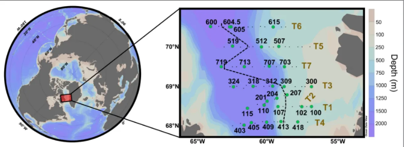
The Green Edge expedition was carried out in Baffin Bay aboard the research icebreaker NGCC Amundsen from 3 June to 14 July 2016 (Figure 1). Baffin Bay is characterized
by a large abyssal plain in the central region (with depths
Figure 1: Location of the sampling stations during the Green Edge expedition. Hydrology, nutrients, and
pigment analysis were performed at all stations (black dots and green circles). The silicon cycle was studied at sta-tions indicated by green circles. Transects T1 to T7 are numbered following their chronological order of sampling. Transects were sampled during the following periods: T1, 9–13 June; T2, 14–17 June; T3, 17–22 June; T4, 24–29 June; T5, 29 June–3 July; T6, 3–7 July; T7, 7–10 July. The black dashed line represents the approximate location of the ice edge at the time of sampling of each transect. Stations located west of this line were covered by sea ice when sampled. DOI: https://doi.org/10.1525/elementa.382.f1
to 2300 m) and continental shelves located on both sides of the bay. The continental shelf off Greenland is wider and ends with an abrupt shelf break. The icebreaker per-formed seven perpendicular transects across the marginal ice zone (MIZ) from the open waters to the sea ice, cover-ing an area from 67°N to 71°N, and from 55°W to 64°W. This sampling strategy was chosen in order to capture every step of the bloom phenology: from a pre-bloom situation under the compact sea ice at the western ends of transects, through the bloom initiation and growth close to the ice edge, to a post-bloom situation at the easternmost open water stations. The number assigned to each transect (T1 to T7) follows the chronological order of sampling. This order was dictated by the optimization of the ship’s route, which was constrained by a mid-cruise changing of the scientific team and sea ice conditions.
Sample collection and analyses Hydrographic data
At each hydrographic station, seawater collection and ver-tical profiles of water column properties were made from an array of 24, 12-L bottles mounted on a rosette equipped with a Seabird SBE-911 plus CTD unit, which also included a Seapoint SCF Fluorometer for detection of chlorophyll
a (Chl a). Close to the rapidly melting marginal ice zone,
density profiles often did not exhibit a well-mixed layer nor a clear density step below; hence we calculated an equivalent mixed layer (hBD) as defined in Randelhoff et al. (2017), used for strongly meltwater-influenced layers in the marginal ice zone (MIZ). Also in accordance with Randelhoff et al. (2019), we defined the depth of the euphotic zone (Ze) as the depth where a daily irradiance of photosynthetically available radiation (PAR) of 0.415 Einstein m–2 d–1 was measured. This value delimits the
lower extent of the vertical phytoplankton distribution in the north Pacific subtropical gyre (Letelier et al., 2004). Based on Green Edge data, Randelhoff et al. (2019) showed that Ze estimated using the 0.415 Einstein m–2 d–1 criteria
was not statistically different from Ze estimated using the more widely-used 1% surface PAR criteria. Vertical profiles of instantaneous downwelling irradiance were measured to a depth of 100 m using a Compact Optical Profiling System (C-OPS, Biospherical Instruments, Inc.). Daily PAR just above the sea surface was estimated using both in situ data recorded on the ship’s meteorological tower and the atmospheric radiative transfer model SBDART (Ricchiazzi et al., 1998). More information about light transmittance in the water column and its measurement methodology (in particular for sea ice-covered stations) can be found in Randelhoff et al. (2019).
Dissolved nutrients
Nutrient (NO3–, PO
43–, H4SiO4) analyses were performed
onboard on a Bran+Luebbe Autoanalyzer 3 using stand-ard colorimetric methods (Grasshoff et al., 2009). Ana-lytical detection limits were 0.03 μmol L–1 for NO
3–, 0.05
μmol L–1 for PO
43– and 0.1 μmol L–1 for H4SiO4.
The Atlantic and Pacific Oceans provide source waters for the Arctic Ocean that can be distinguished by their dif-fering nitrate and phosphate concentration relationship. Following Jones et al. (1998), the ‘Arctic N-P’ tracer (ANP)
was calculated for each station. It quantifies the propor-tion of Atlantic and Pacific waters in a water body using their N-P signatures. Essentially, ANP = 0% means the NO3–/PO
43– pairs fall on the regression line for Atlantic
waters, whereas ANP = 100% means the NO3–/PO
43– pairs
fall on the regression line for Pacific waters. Because the ANP index is a ratio, it is a quasi-conservative water mass tracer and is not influenced by the biological consump-tion of nutrients. The limit between ‘Pacific’ vs ‘Atlantic’ influenced waters was placed arbitrarily at stations where the ANP = 25%.
Pigments
For pigment measurements, <2.7 L seawater samples were filtered on Whatman GF/F filters and stored in liquid nitrogen until analysis. Back at the laboratory, all samples were analyzed within three months. Filters were extracted in 100% methanol, disrupted by sonication, and clarified by filtration (GF/F Whatman) after 2 h. Samples were analysed within 24 h using High Performance Liquid Chromatography on an Agilent Technologies HPLC 1200 system equipped with a diode array detector following Ras et al. (2008).
Sea ice satellite data
Sea ice concentrations (SIC) have been extracted from AMSR2 radiometer daily data on a 3.125 km grid (Beitsch et al., 2014). At each station, the SIC was extracted from the closest pixel using the Euclidian distance between the ship position and the centre of each pixel. The SIC is an index that ranges between 0 (complete open water) and 1 (complete ice cover). Here, we placed the ice-edge limit at stations with SIC = 0.5. Based on SIC history, we also retrieved the number of days between the sampling day and the day at which SIC dropped below 0.5 (DOW50) to estimate the timing of the melting of sea ice. DOW50 can take positive or negative values, depending if SIC at the time of sampling is >0.5 (DOW50 negative) or <0.5 (DOW50 positive).
Description of the diatom bloom Particulate silica concentrations
Biogenic (BSi) and lithogenic (LSi) silica concentrations were measured at 29 stations covering the seven transects (Figure 1). Samples were taken at 7 to 14 depths between
0 and 1674 m depth. For each sample, 1 L of seawater was filtered onto 0.4 μm Nucleopore polycarbonate filters. Filters were then stored in Eppendorf vials, and dried for 24 h at 60°C before being stored at room temperature. Back at the laboratory, BSi was measured by the hot NaOH digestion method of Paasche (1973) modified by Nelson et al. (1989). After NaOH extraction, filters were assayed for LSi by HF addition for 48 h using the same filter.
Biogenic silica uptake rates (ρSi)
Biogenic Si uptake rates (ρSi) were measured by the 32Si
method (Tréguer et al., 1991; Brzezinski and Phillips, 1997) for 21 stations at 5 to 7 different depths, corre-sponding to different levels of PAR, ranging from 75 to 0.1% of surface irradiance. At the ice-covered stations, samples that were collected under the ice were incubated
in the same way as the samples collected in open waters, because onboard we only had access to the light transmit-tance through the water column that did not take into account attenuation through the ice. However, at three stations (201, 403, and 409) we were able to perform two incubation experiments in parallel that either did or did not take into account the light attenuation through the ice. Due to light attenuation at depth, this affects only the first 20 m where we have estimated a mean bias in our ρSi measurement under the ice of 0.005 ± 0.003 μmol L–1 d–1 (i.e. 23 ± 9% difference), which should not change
substantially the interpretation of the main results, but would have to be taken into account if our data are used to constrain a regional Si budget.
The following equation was used to calculate Si uptake rates:
[
4 4]
H SiO 24 Si Af Ai T ρ = × ×where Af is the final activity of the sample, Ai the initial activity, and T the incubation time (in hours). Briefly, poly-carbonate bottles filled with 160 mL of seawater were spiked with 667 Bq of radiolabeled 32Si-silicic acid
solu-tion (specific activity of 18.5 kBq μg-Si–1). For most of the
samples, H4SiO4 addition did not exceed 1% of the initial concentration. Samples were then placed in a deck incu-bator cooled by running sea surface water and fitted with blue plastic optical filters to simulate the light attenu-ation of the corresponding sampling depth. After 24 h, samples were filtered onto 0.6 μm Nucleopore polycar-bonate filters and stored in a scintillation vial until further laboratory analyses. 32Si activity on filters was measured
in a Packard 1600 TR scintillation counter by Cerenkov counting following Tréguer et al. (1991). The background for the 32Si radioactive activity counting was 10 cpm.
Sam-ples for which the measured activity was less than 3 times the background were considered to lack Si uptake activity. The specific Si uptake rate VSi (d–1) was calculated by
nor-malizing ρSi by BSi.
Taxon-specific contribution to biogenic silica production (PDMPO)
Taxon-specific silica production was quantified using the fluorescent dye PDMPO, following Leblanc and Hutchins (2005), which allows quantification of newly deposited Si at the specific level in epifluorescence microscopy. Com-pared to confocal microscopy, this technique allows analy-sis of a large number of cells and therefore gives a robust estimation of the activity per taxon. Although images are acquired in two dimensions, superimposed fluorescence in the vertical plane increases the fluorescence in the x–y plane and reduces measurement biases. Briefly, 170 mL of seawater samples were spiked onboard with 0.125 μmol L–1 PDMPO (final concentration) and incubated in the
deck incubator for 24 h. The samples were then centri-fuged down to a volume of 2 mL, resuspended with 10 mL methanol, and then kept at 4°C. At the laboratory, samples were mounted onto permanent glass slides and stored at –20°C before analysis. Microscope slides were
then observed under a fluorescence inverted microscope Zeiss Axio Observer Z1 equipped with a Xcite 120LED source and a CDD black and white AxioCam-506 Mono (6 megapixel) camera fitted with a filter cube (Ex: 350/50; BS 400 LP; Em: 535/50). Images were acquired sequen-tially in bright field and epifluorescence, in order to improve species identification for labelled cells. PDMPO fluorescence intensity was quantified for each taxon fol-lowing Leblanc and Hutchins (2005) using a custom-made IMAGE J routine on original TIFF images. The taxon-spe-cific contributions to silica production were estimated by multiplying, for each taxon, the number of fluorescent cells by the mean fluorescence per cell.
Diatom identification and counting
Seawater samples collected with the rosette at discrete depths were used for diatom identification and quantita-tive assessment of diatom assemblages. Prior to counting, diatom diversity was investigated at three stations using a Phenom Pro scanning electron microscope (SEM) (See Figure S1 for SEM pictures illustrating the key species). For SEM analysis, water samples were filtered (0.25–0.5 L) onto polycarbonate filters (0.8 μm pore size, What-man), rinsed with trace ammonium solution (pH 10) to remove salt water, oven-dried (60°C, 10 h) and stored in Millipore PetriSlides. Pictures were taken at magnifica-tion up to × 25,000.
Cell counts were done within a year after the expedi-tion. Samples were regularly checked and lugol was added when needed. In total, 43 samples were analysed from 25 stations (Figure 1): 23 were collected at the near surface
(0–2 m depth), and 20 were collected at the depth of the subsurface chlorophyll a maximum (SCM) when the max-imum of Chl a was not located at the surface. Aliquots of 125 mL were preserved with 0.8 mL acidified Lugol’s solution in amber glass bottles, then stored in the dark at 4°C until analysis. Counting was performed in the labo-ratory following Utermöhl (1931) using a Nikon Eclipse TS100 inverted microscope. For counting purposes, mini-mum requirements were to count at least three transects (length: 26 mm) at ×400 magnification and at least 400 planktonic cells (including Bacillariophyceae, but also Dinophyceae, flagellates, and ciliates). Raw counts were then converted to number of cells per litre. In this paper, only data on diatom counting are presented.
Conversion to carbon biomass
Diatom-specific C biomass was assessed following the methodology of Cornet-Barthaux et al. (2007). Except for rare species, cell dimensions were determined from rep-resentative images of each of 35 taxa, where the mean (± standard deviation) number of cells measured per taxon was 21 (±14) (see Table S1). Measuring the three dimen-sions of the same cell is usually difficult. When not visible, the third dimension was estimated from dimension ratios documented in European standards (BS EN 16695, 2015). For each measured cell, a biovolume was estimated using linear dimensions in the appropriate geometric formula reflecting the cell shape (BS EN 16695, 2015). A mean bio-volume was then estimated for each taxon and converted
to carbon content per cell according to the corrected equation of Eppley (Smayda, 1978), as follows:
(
)
Log C biomass 0.76 Log cell volume= −0.352
C content per cell (pg cell–1) was multiplied by cell
abun-dance (cells L–1) to derive total carbon biomass per taxon,
expressed in units of μg C L–1. Statistical analyses
Diatom assemblage structures were investigated through cluster analysis (Legendre and Legendre, 2012). Abun-dance data were normalized by performing a Log (x + 1) transformation. Euclidean distances were then calculated between each pair of samples, and the cluster analysis was performed on the distance matrix using Ward’s method (1963). Cluster analysis based on Bray-Curtis similarities gave the same clusters. The output dendrogram displays the similarity relationship among samples. An arbitrary threshold was applied to separate samples into compact clusters. A post hoc analysis of similarity (one-way ANO-SIM) was performed to determine whether clusters dif-fered statistically from each other in terms of taxonomic composition.
Trait-based analysis
A trait-based analysis was performed following Fragoso et al. (2018) to identify functional traits that determine species ecological niches (data used are listed in Table S2). Briefly, eight diatom traits were selected according to their ecological relevance and availability of information in the literature: equivalent spherical diameter (ESD); sur-face area to volume ratio (S/V); optimum temperature for growth (Topt); ability to produce ice-binding proteins (IBP);
the presence or absence of long, sharp projections such as setae, spines, horns and cellular processes (spikes); degree of silicification, qualitatively based on examination of SEM images (silicified); the propensity to form resting spores (spores); and the ability to form colonies (colonies). More detailed description of the traits can be found in Fragoso et al. (2018). Due to the difficulty of finding infor-mation about every trait for every diatom species, only the dominant taxa were included in the analysis and some species were grouped on the basis of trait similarities. A community-weighted trait mean (CWM) is an index used to estimate trait variability on a community level. CWM values were calculated for each trait in each sample from two matrices: a matrix that gives trait values for each spe-cies, and a matrix that gives the relative abundances for each species in each sample. CWM is calculated according to the following equation:
s i 1 CWM p xi. i = =
∑
where S is the number of species in the assemblage, pi is the relative abundance of each species, and xi is the species-specific trait value. Each of the eight traits was normalized in relation to the stations that presented the lowest (= 0) and the highest values (=1).
Results
Environmental conditions Ice cover and water masses
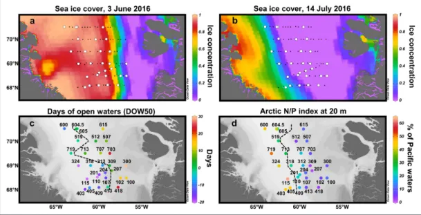
As shown in Figure 2a, b depicting sea ice
concentra-tions, the expedition was marked by the westward retreat of the sea ice in Baffin Bay (all data and metadata are summarized in Table S3). Just before the beginning of the
Figure 2: Hydrographic conditions in central Baffin Bay during June–July 2016. (a–b) Five-day composite images
of sea ice concentrations. White circles correspond to the stations where the silicon cycle was studied. (c) Number of
days since the sea ice concentration dropped below 0.5 (DOW50). The black dashed line corresponds to the approxi-mate location of the ide edge at the time of sampling (i.e., where DOW50 = 0). (d) Fraction of Pacific waters at 20 m
(ANP index). The black dashed line delimits the Pacific-influenced waters (ANP > 25%) from the Atlantic-influenced waters (ANP < 25%). DOI: https://doi.org/10.1525/elementa.382.f2
expedition (3 June), most of the stations where the sili-con cycle was studied were covered by sea ice, whereas at the end of the expedition (14 July), all were ice-free, with the exception of station (st.) 719. A composite picture of DOW50 at each site at the time of sampling is presented in
Figure 2c. The retreat of the melting sea ice towards the
west was more pronounced during the last three transects (T5–T7) as shown by the ice-edge position (located where DOW50 = 0 and SIC = 0.5). West of this limit, stations were covered by sea ice (SIC > 0.5) when sampled, whereas to the east, the sea ice had already melted (SIC <0.5) since a number of days ranging from 0 (st. 605) to 31 (st. 300).
Using the Arctic N-P relationship calculated from nutrient samples collected at 20-m depth, the frac-tion of Pacific waters in the water samples increased westwards (Figure 2d), in accordance with the global
circulation pattern established for Baffin Bay. Most of the eastern stations exhibited an ANP <15%, whereas ANP increased significantly from the middle of the bay to the westernmost stations, reaching 63% at st. 115. Atlantic- and Pacific-influenced waters (delimited by ANP = 25%) were also associated with wide differences
in salinity, temperature and density profiles in the upper layer (Figure S2). According to Tang et al. (2004), these wide differences are due to the warm and salty inflow of the West Greenland Current from the eastern side of Davis Strait (entailing Atlantic-influenced waters to the east) and the cold and fresh outflow from the Canadian Archipelago and water masses produced within Baffin Bay (entailing Pacific-influenced waters to the west). The warm current along the west coast of Greenland also explains why the sea ice melts toward the west in Baffin Bay (Tang et al., 2004), whereas in the other Arctic regions, it usually melts northward (Perrette et al., 2011).
Nutrient distribution
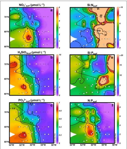
The distribution of nutrients (Figure 3) in surface waters
was characterized by a decreasing west-to-east gradient that generally followed the ice coverage at the time of sampling. Overall, surface concentrations were higher at stations covered by sea ice (maximum concentrations: [H4SiO4] = 9.2 μmol L–1; [NO
3–] = 5.9 μmol L–1; [PO43–] = 0.9
μmol L–1). In contrast, at open-water stations located east
of the ice edge, nutrients were close to exhaustion,
some-Figure 3: Surface nutrient concentrations and potential limiting nutrients. Concentrations of surface nitrate (a),
orthosilicic acid (b), and phosphate (c) in μmol L–1. Molar ratios of Si:N (d), Si:P (e), and N:P (f) at the surface. The
black dashed lines correspond to the approximate location of the ice edge. The white circles correspond to the sta-tions where the silicon cycle was studied. DOI: https://doi.org/10.1525/elementa.382.f3
times near detection limits (0 < [H4SiO4] < 1.4 μmol L–1; 0
< [NO3–] < 0.7 μmol L–1; 0 < [PO
43–] < 0.2 μmol L–1), except
for stations 605 and 604.5 where nutrient concentrations were similar to the ice-covered stations. For the southern transects (T1–T4) and T5, nutrient depletion extended well inside the ice pack. The vertical distribution of nutri-ents along transects (Figure S3) indicated that depletion extended to greater depths towards the east, especially for orthosilicic acid which was depleted down to 60-m depth. The west-east gradient observed at the surface was also found when nutrients were integrated over the depth of the equivalent mixed layer (Supplemental Figure S4).
The nutrient ratios Si:N:P = 16:16:1 derived from Redfield et al. (1963) and Brzezinski (1985) can be used to determine the potential limiting nutrients for dia-toms. Overall, in surface waters (Figure 3d–f) and down
to 20–30 m (Figure S5), Si:N > 1, Si:P < 16 (except on the eastern part of T2, T3 and T5) and N:P < 16, indicating that NO3– was the first potentially limiting nutrient,
fol-lowed by H4SiO4 and PO43–. Nitrate limitation (Figure 3d)
was much more pronounced in the eastern half of the bay because nitrate concentrations were close to zero. At 40-m depth (Figure S5), Si:N was generally lower than 1 on the eastern side of the bay, indicating a potential silicic acid limitation in those subsurface waters.
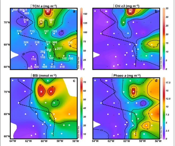
Integrated proxies of protist biomass
The TChl a standing stock, an indicator of algal biomass, was integrated over 80-m depth (Figure 4a). Values were
highest at st. 615 (164.4 mg m–2; up to 12.8 μg L–1 at 26 m),
in the northeast of the sampling area. High values were also observed in the eastern parts of T1–T3 (between 44.3 and 100.7 mg m–2; up to 3.5 μg L–1 at st. 207 at 15 m), and
in the middle of T5–T7 (>71.9 mg m–2; up to 9.6 μg L–1 at
st. 512 at 20 m). Integrated TChl a was lower in the rest of the studied area (between 5.5 and 48.0 mg m–2), especially
on the western side and throughout T4. Vertical sections (Figure S3) show that the TChl a distribution was mainly located within the subsurface maximum that deepened to 60-m depth at the easternmost stations, characterizing late bloom conditions.
The chlorophyll-c3 (Chl c3) pigment was used as a diag-nostic pigment for Phaeocystis spp. biomass instead of the more traditionally used 19′Hexanoyloxyfucoxanthin, as the latter has been shown to be absent in arctic Phaeocystis strains (Antajan et al., 2004; Stuart et al., 2000). A signif-icant linear relationship (R2 = 0.74; p < 0.0001; n = 36)
was obtained between Chl c3 concentrations (in μg L–1)
and Phaeocystis spp. abundances determined by micro-scopic counts (Figure S6). When integrated over 80-m depth (Figure 4b), the highest Chl c3 standing stock was
Figure 4: Depth-integrated phytoplankton pigments and BSi throughout the study area. Distribution of
depth-integrated TChl a (a), Chl c3(b), BSi (c), and Phaeophorbide a (d). Vertical integrations were made from the
surface to 80 m, because at that depth almost all Chl a profiles were sufficiently close to 0, indicating that no signifi-cant biomass was missed. The black dashed lines correspond to the approximate location of the ice edge at the time of sampling. White circles indicate the stations where the silicon cycle was studied. Integrated pigments (a, b and d) are expressed in mg m–2 and BSi (c) in mmol m–2. DOI: https://doi.org/10.1525/elementa.382.f4
observed at st. 615 (35.5 mg m–2) and matched the
subsur-face Chl a peak. High amounts of Chl c3 were also found at st. 512 (16.9 mg m–2) and 300 (17.4 mg m–2). At these
stations (except for st. 512), the Chl c3:TChl a ratio reached values equal to or slightly higher than 0.20 (up to 0.23), which is typical of Phaeocystis species (Antajan et al., 2004; Stuart et al., 2000).
At st. 615, integrated BSi over 80-m depth (Figure 4c)
was low (27.2 mmol m–2) compared to the other stations
located east of the ice edge. Throughout the area, two BSi accumulation areas were observed, located at stations 507 and 512 (reaching 79.6 mmol m–2) and at stations 207,
300, 309 (reaching 63.4 mmol m–2) (see next section for
details of vertical distribution).
Phaeophorbide a is a degradation product of Chl a (Figure 4d) and is indicative of grazing. When integrated
over 80-m depth, low standing stocks were observed throughout section T7 and at the western sea ice-covered stations (<4.4 mg m–2), except for stations located close
to the ice edge on sections T1–T4. Along these transects, moderate to high phaeophorbide a standing stocks (>4.5 mg m–2) were measured from right below the ice edge to
the end of the transect to the east, with maximum values
at st. 102 (14.3 mg m–2) and st. 413 (11.6 mg m–2). For
sections T5 and T6, standing stocks started to increase far from the ice edge, with a maximum throughout the studied area observed at st. 507 (18.9 mg m–2).
Vertical distribution of particulate silica and BSi uptake rates
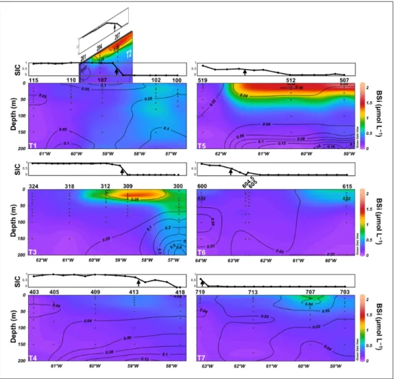
Particulate silica concentrations
Throughout the study area, very low BSi concentra- tions (<0.49 μmol L–1) were observed at stations covered
by sea ice (Figure 5), except for a few stations located
close to the ice edge (e.g. stations 312 and 204). This effect is particularly obvious on T4, a transect which was almost completely covered by sea ice at the time of sampling. In contrast, highest concentrations were observed east of the ice edge, on transects T5 ([BSi]max = 1.89 μmol L–1 at st.
512, [BSi]max = 2.15 μmol L–1 at st. 507), T2 ([BSi]
max = 1.70
μmol L–1 at st. 207) and T3 ([BSi]
max = 2.01 μmol L–1 at st.
309). On T5, BSi was accumulated mainly in the upper 30 m, whereas on T3, the peak of BSi was first located within the upper 30 m (stations 312 and 309), then extended downward to depths of 90–180 m at the easternmost st. 300, with moderate concentrations (0.47–0.57 μmol L–1).
Figure 5: Vertical distribution of biogenic silica concentrations along the seven transects. Biogenic silica (BSi)
is expressed in μmol L–1. Contour lines represent lithogenic silica (LSi), expressed in μmol L–1. Sea ice concentrations
(SIC) are shown in the graph above each transect. The black arrow in those graphs indicates the location of the ice edge (SIC = 0.5). DOI: https://doi.org/10.1525/elementa.382.f5
The BSi accumulation area observed at stations 309, 204 and 207 decreased in intensity southward but was still vis-ible in the eastern part of T1 (st. 102), also characterized by moderate BSi concentrations (0.47–0.61 μmol L–1) to
150-m depth. BSi distribution along T6 and T7 followed a different pattern, with low concentrations (<0.53 μmol L–1), except in very specific areas (stations 615 and 707)
located far from the ice edge, where moderate concentra-tions (up to 0.89 μmol L–1) were measured.
The vertical distribution of LSi (Figure 5) indicated low
concentrations (<0.15 μmol L–1) at every station, except at
st. 300 where LSi reached 0.74 μmol L–1 at 180-m depth,
which is probably a result of proximity to the seabed. This station was located on the Greenland shelf, and charac-terized by a relatively shallow bottom depth of 196 m. Ragueneau and Tréguer (1994) showed that a fairly con-stant percentage of siliceous lithogenic material (up to 15% for a coastal environment) can dissolve during the first alkaline digestion, resulting in an overestimation of BSi when water samples are enriched with LSi. However, using this upper 15% value, we estimate that the LSi interference was less than 0.025 μmol L–1 for most of our
samples. Corresponding BSi concentrations were always much higher, even at st. 300 where LSi contamination
could have reached 0.11 μmol L–1. In addition, plotting LSi
versus BSi did not yield a significant linear relationship (r = 0.04; p = 0.44), suggesting that LSi concentrations were too low to significantly bias our BSi measurements.
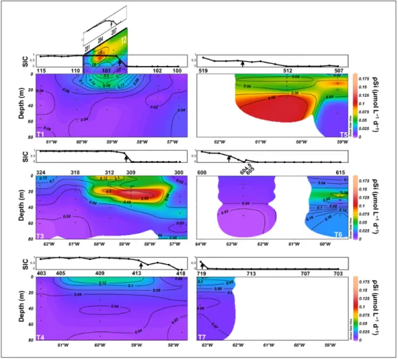
Biogenic silica uptake rates
Si uptake rates (ρSi) (Figure 6) generally followed the
BSi distribution, with lower ρSi at the westernmost ice-covered stations and highest values centred around the two BSi accumulation areas located on T2, T3, and T5. The highest ρSi was located at st. 309 at 20-m depth (0.19 μmol L–1 d–1). Si uptake rates were also high at stations
312 (up to 0.10 μmol L–1 d–1) and 204 (up to 0.12 μmol L–1
d–1), which were covered by sea ice but located close to the
ice edge. On transect T5, the highest Si uptake rate (0.10 μmol L–1 d–1) at st. 507 matched the peak of BSi (2.15 μmol
L–1) located at 12-m depth, whereas at st. 512, the peak of
Si uptake was located below the peak of BSi (ρSimax = 0.12 μmol L–1 d–1 at 30 m; BSi
max = 1.89 μmol L–1 at 15 m). Si
uptake was low throughout transects T4 and T1 (<0.02 μmol L–1 d–1) except below the sea ice at stations 107 and
409 where ρSi was moderate (0.05–0.06 μmol L–1 d–1).
Along T6, a local peak of production (0.10 μmol L–1 d–1)
was measured at st. 615 at 25-m depth, matching both the
Figure 6: Vertical distribution of Si uptake rates along the 7 transects. Si uptake rate (ρSi, in μmol L−1 d−1) was
measured from the surface to the depth at which 0.1% of the surface PAR remained. Contour lines represent the spe-cific Si uptake rate (VSi, in day−1). Sea ice concentrations (SIC) are shown in the graphs above each transect. The black
arrow in those graphs indicates the location of the ice edge (SIC = 0.5). For T5–T7, ρSi and VSi were not interpolated throughout the transect because of lack of data. DOI: https://doi.org/10.1525/elementa.382.f6
SCM and BSi maximum measured at this station. Station 719, which was located close to the ice edge of T7 was characterized by very low ρSi values (<0.03 μmol L–1 d–1).
Specific Si uptake rates (VSi) (Figure 6) were clearly
higher below the sea ice at stations close to the ice edge (0.11–0.16 d–1 at stations 204, 312, 409, and 719), with a
maximum observed at st. 107(0.23 d–1). Stations 204 and
312 were associated with high BSi concentrations, indicat-ing that the biomass had had time to accumulate, whereas BSi was still low at stations 107, 409, and 719, which could be indicative of an early bloom stage. On T5, VSi was low at the easternmost st. 507 (<0.05 d–1), whereas a
subsur-face maximum was measured at st. 512 (0.10 d–1 at 30 m),
matching the ρSi peak. On T6, VSi was low at st. 604.5 (<0.05 d–1), but two subsurface VSi peaks were measured
at st. 615 (0.12 d–1 at 25 m; 0.20 d–1 at 50 m). Diatom assemblage structure
Absolute abundance and carbon biomass
In total, 47 diatom taxa were identified to the species or genus level in this study. The taxa are listed in Table S4.
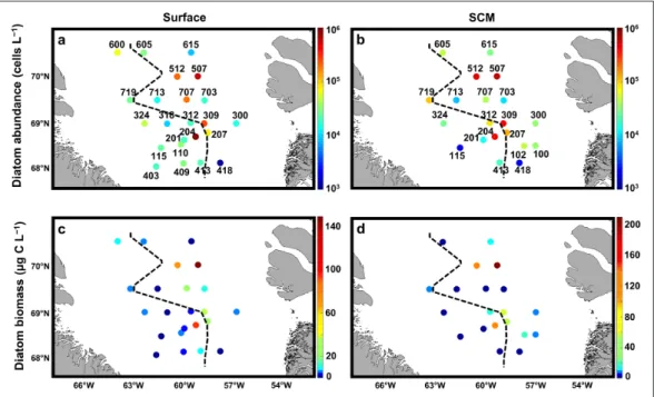
Diatom abundance (Figure 7a, b) was highly variable
throughout the study area, ranging in surface waters from 1,000 cells L–1 at st. 418 to 916,000 cells L–1 at st.
204, the latter being covered by sea ice (SIC = 0.93) but located close to the ice edge. As a general tendency, higher abundances were found at ice-free stations (185,000 to 624,000 cells L–1, at stations 309, 507, 512, and 707), and
closely matched the two BSi accumulation areas (Figures 4c and 5). Abundances were low to moderate (<79,000
cells L–1) for the other stations, independently of ice
cover. The depth of the TChl a maximum varied among stations, and was located between the surface and 44 m. At the SCM, diatom abundances followed a pattern of distribution similar to that observed at the surface, with
higher abundances observed on transect T5 (484,000 and 610,000 cells L–1 at stations 507 and 512), and close to the
ice edge of transects T2 and T3 (119,000 to 464,000 cells L–1 at stations 204, 207, and 309), both on the western and
eastern sides of this limit.
Total diatom carbon biomass (Figure 7c, d) for surface
and SCM varied, respectively, from 0.1 (st. 418) to 149.0 μg C L–1 (st. 507) and from 0.1 (st. 418) to 210.0 μg C L–1
(st. 507). Throughout the study area, most of the stations exhibited low to very low carbon biomass (<20.0 μg C L–1),
with the exception of stations 204, 207, 309, 507, and 512, both at the surface (75.1 ± 49.3 μg C L–1, n = 5) and at the
SCM (116.1 ± 64.2 μg C L–1, n = 5). Station 707 was
char-acterized by an intermediate diatom carbon biomass (25.3 μg C L–1), but only at the surface.
Relative abundance and carbon biomass
Regarding cell numbers, the five taxa that dominated the diatom assemblages were (Figure 8a, b): Chaetoceros
spp. (mean ± sdv for the 43 samples counted: 19 ± 26%; mostly C. gelidus and C. decipiens), Pseudo-nitzschia spp. (17 ± 23%), Ceratoneis closterium (14 ± 16%),
Fragilariop-sis spp./Fossula arctica (13 ± 16%), and Thalassiosira spp.
(9 ± 9%; mostly T. antarctica var. borealis, T. gravida, and T.
nordenskioeldii). Fragilariopsis spp. and Fossula arctica were
grouped together because of the difficulty in distinguish-ing the two taxa with light microscopy in some samples.
At the surface, a distinct diatom assemblage was located within the main BSi accumulation areas (stations 204, 207, 300, 309, 507, 512, 703, and 707; Figure 4c). These
stations (n = 8) were characterized by a larger contribution of Chaetoceros spp. (56 ± 18%) and also by a moderate proportion of Thalassiosira spp. (12 ± 7%). In contrast, at the other surface stations (n = 15), the diatom assemblage was dominated by Ceratoneis closterium (26 ± 19%) and by
Figure 7: Absolute diatom abundance and carbon biomass. Live diatom cell abundance (cell L–1) at the surface (a)
and the subsurface chlorophyll a maximum (SCM) (b). Live diatom carbon biomass (μg C L–1) at the surface (c) and
the SCM (d). The black dashed lines correspond to the approximate location of the ice edge at the time of sampling.
Fragilariopsis spp./Fossula arctica (20 ± 19%). The
follow-ing ice-associated species were also observed at the sur-face: Melosira arctica vegetative cells (13 ± 10% at stations 110, 201, 413, and 409), Synedropsis antarctica (7 ± 3% at stations 318, 403, 409, and 600), and Nitzschia frigida (4 ± 3% at stations 110, 204, 318, 409, 207, 309, and 512).
At the SCM, two distinct diatom assemblages were also observed. Similarly to the surface, one assemblage was located where a diatom bloom was taking place (sta-tions 204, 207, 309, 312, 507, and 512) or probably had occurred (stations 100, 102, and 300), according to BSi and ρSi data (Figures 5 and 6). This assemblage (n = 9) was also characterized by a larger proportion of Chaetoceros spp. (37 ± 18%) and variable proportions of Fragilariopsis spp./Fossula arctica (19 ± 13%) and Thalassiosira spp. (18 ± 8%). Excluding stations 115 and 418 where diatom abundances were extremely low, the other SCM stations (n = 9) were largely dominated by Pseudo-nitzschia spp. (56 ± 17%) and by some unidentified pennate diatoms (16 ± 16%).
On two occasions, Melosira arctica resting spores con-tributed importantly to relative abundance: at stations 512 (surface: 20%; SCM: 26%) and 703 (SCM: 17%). Although we had not expected to observe such a high contribution
of an ice-associated diatom at st. 703 (DOW50 = 23 days), it represents only 1.8 × 10³ spores L–1 in terms of absolute
abundances, as diatom abundances at this station were very low. Melosira spp. resting spores were also observed with a contribution <6% at stations 312, 318, 413, 207, and 507. Resting spores of Thalassiosira antarctica var.
borealis (data not shown) were rare but were identified at
stations 100, 102, and 615 (up to 3.0 × 10³ spores L–1).
When converted to carbon biomass (Figure 8c, d), the
contribution of centric diatoms increased at all stations, even at some stations where pennate diatoms largely dominated in terms of abundances. This increase is par-ticularly obvious for Thalassiosira spp., which accounted for 21 ± 17% of diatom C biomass at the surface taking into account all of the stations (n = 23), and 41 ± 29% at the SCM (n = 20), but also for Melosira arctica vegeta-tive cells (26 ± 15% at the surface of stations 110, 201, 409 and 413). Chaetoceros spp. C biomass accounted for 19 ± 26% at the surface (n = 23) and 10 ± 14% at the SCM (n = 20), and was largely associated with the main diatom accumulation areas. Conversely, pennate diatoms such as
Ceratoneis closterium and Fragilariopsis spp./Fossula arc-tica, which were key contributors to one of the two
assem-blages observed at the surface, accounted for a much lower
Figure 8: Relative diatom abundance and carbon biomass. Relative abundance (%) of each diatom taxon at the
surface (a) and the subsurface chlorophyll a maximum (SCM) (b). Relative carbon biomass (%) of each taxon at
the surface (c) and the SCM (d). The station numbers for ice-covered locations (SIC > 0.5) are indicated in blue font
biomass at those same stations (respectively, 13 ± 11% and 7 ± 8%, n = 15), due to their lower biovolumes. This trend was also true for Pseudo-nitzschia spp., a taxon that was observed to dominate one of the two assemblages at the SCM, and had a low contribution to C biomass at those same stations (11 ± 7%, n = 9). The category ‘Other species’ which is composed of rare (i.e., Rhizosolenia spp.,
Coscinodiscus spp., Porosira glacialis, Entomoneis spp., Bacterosira bathyomphala, etc.) and mostly large taxa, was
important in terms of diatom C biomass at some stations, with up to 18% in the surface at st. 707.
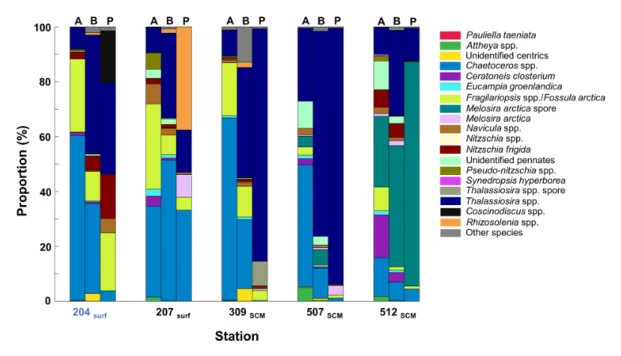
Taxon-specific contributions to silica production
The contribution of each taxon to biogenic silica pro-duction was investigated using PDMPO epifluorescence image analysis (see Figure S7 for illustrations) for the five most productive stations (i.e., with the highest ρSi) in order to identify the most actively silicifying species at locations where a diatom bloom was taking place. For those stations, relative abundance, biomass and species-specific silicification contributions have been presented together for comparison (Figure 9). Thalassiosira spp.
(mostly T. antarctica var. borealis and T. gravida) strongly dominated BSi production at the SCM at stations 309 and 507 (respectively, 85 and 93%). At these stations,
Thalas-siosira spp. contributions increased successively between
abundance (respectively, 9 and 27%), C biomass (respec-tively, 40 and 75%), and Si production. Conversely,
Chae-toceros spp. (mostly C. gelidus) were major contributors to
cell abundance (up to 60%), but were negligible in terms of BSi production, due to their small biovolume and weak degree of silicification. The fluorescence of C. gelidus was often low and difficult to detect, such that some labelled
C. gelidus cells may have been missed, but an
under-esti-mation would not have affected our results significantly, as fluorescence per C. gelidus cell was much lower than the fluoresence of the other taxa. Melosira arctica resting spores were actively silicifying at the SCM at st. 512, con-tributing 82% of Si production, while they contributed only 26% of abundance and 44% of C biomass.
Chae-toceros spp., mostly C. decipiens, were very active in the
surface at st. 207(32%) and also important contributors to both abundance (33%) and biomass (51%). Two very rare taxa contributed significantly to Si production in two surface locations: Coscinodiscus spp. (19%) at st. 204 and
Rhizosolenia spp. (38%) at st. 207. Due to a large surface
area, Coscinodiscus spp. were characterized by the high-est silicifying activity per cell (i.e., PDMPO fluorescence).
Fragilariopsis spp./Fossula arctica were actively silicifying
mainly in the surface at ice-covered st. 204 (21%), while they were also important contributors to abundance in the surface at st. 207 and at the SCM at St. 309. The sea ice diatom Nitzschia frigida was only found active in the surface at the ice-covered station 204 (16%).
Discussion
During the Green Edge expedition, the development of the late spring–early summer diatom bloom was stud-ied in relation with the sea ice retreat. Through this study, we have attempted to fully describe the diatom bloom dynamics in central Baffin Bay, by describing diatom assemblage structures and carbon biomass, and silica uptake activities at both the assemblage and the genus/species level. A cluster analysis, performed to sum-marize the main results (Figures 10 and 11, Table 1), is
discussed in the following sections.
Figure 9: Taxon-specific contribution to biogenic silica deposition at the five most productive stations. For
each station, relative abundance (A), carbon biomass (B) and PDMPO fluorescence (P) are presented for comparison. Station 204 was covered by the ice pack (SIC > 0.5). The taxa Coscinodiscus spp., and Rhizosolenia spp., as well as spores of Thalassiosira spp. were extracted from the category ‘Other species’ in order to show their importance in terms of contribution to BSi deposition. DOI: https://doi.org/10.1525/elementa.382.f9
Characterization of the diatom bloom: Development in relation with the hydrographic conditions
The cluster analysis (Figure 10a, b) performed separately
on surface and SCM abundance data identified four clus-ters of stations. ANOSIM one-way analysis compared each pair of clusters and showed that clusters 1 and 2 were not statistically different from clusters 1′ and 2′, respectively (p-values from pairwise analyses were equal, respectively, to 0.08 and 0.38). Hence, hereafter we will only distin-guish the two statistically different clusters 1/1′ and 2/2′, which were observed both at the surface and the SCM.
The cluster 2/2′ stations were associated with the highest integrated Chl a and BSi measured in Baffin Bay (81.5 ± 29.0 mg m–2 and 56.1 ± 18.5 mmol m–2,
respec-tively) (Table 1). Integrated Si uptake rates indicate that
this diatom assemblage was actively silicifying (1.70 ±
0.93 mmol m–2 d–1), except at the easternmost stations
100, 102, and 300, where ρSi was low and BSi was moder-ate down to 180-m depth, suggesting a post-bloom stage with diatoms that were probably settling out of the upper mixed layer. Cluster 2/2′ was associated on average with a much higher contribution to total particulate organic carbon (POC) than cluster 1/1′ (Table 1). Cluster 2/2′
represented on average 22% of POC, while cluster 1/1′ only represented 3% of POC. The record contribution of diatoms to C biomass was reached at st. 507, contribut-ing as much as 41% of POC at the surface and 66% at the SCM. Hence, depending on the station, diatoms of clus-ter 2/2′ were either actively blooming or corresponded to a remnant bloom that had occurred a few days or a few weeks before sampling. The cluster 2/2′ stations were mainly located east of the ice edge on transects T1–T3 and
Figure 10: Cluster analysis performed on abundance data from surface and subsurface chlorophyll a maximum samples. The dendrogram displays the similarity relationship among samples in terms of their
taxo-nomic composition, for the surface (a) and the subsurface chlorophyll a maximum (SCM) (b). Map of the study area
with the stations colored according to the cluster they belong to (blue for clusters 1 and 1′; red for clusters 2 and 2′), for the surface (c), and the SCM (d). The black dashed lines correspond to the approximate location of the ice edge
at the time of sampling. (e) Relative abundance and relative carbon biomass for the ‘mean’ assemblages associated
with the two clusters. Clusters 1 and 2 were not statistically different from, respectively, clusters 1′ and 2′ and were therefore grouped together, giving clusters 1/1′ and 2/2′. DOI: https://doi.org/10.1525/elementa.382.f10
T5 (Figure 10c, d), in waters where the sea ice was at an
advanced state of melting (SIC = 0.19 ± 0.36; DOW50 = 5 ± 9 days) and with shallower euphotic zone depths (Ze)
(Table 1). This observation is in accordance with the
clas-sical picture of an Arctic ice-edge phytoplankton bloom starting as a band along the ice edge and developing in
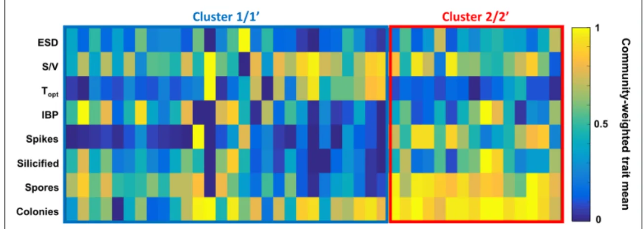
Figure 11: Community-weighted trait means of diatom species found in cluster 1/1′ and 2/2′. The color bar
indicates the value of the normalized community-weighted trait means (0 to 1) for clusters 1/1′ (framed in blue) and 2/2′ (framed in red). The eight traits include equivalent spherical diameter (ESD), surface area to volume ratio (S/V), optimum temperature for growth (Topt), ability to produce ice-binding proteins (IBP), presence or absence of long, sharp projections such as setae, spines, horns and cellular processes (‘spikes’), degree of silicification (‘silicified’) quali-tatively based on examination of SEM images, propensity to form resting spores (‘spores’), and ability to form colonies (‘colonies’). Each trait was normalized in relation to the stations that presented the lowest (= 0) and the highest values (=1). DOI: https://doi.org/10.1525/elementa.382.f11
Table 1: Mean and standard error of hydrographic and biological parameters for each cluster. DOI: https://doi.
org/10.1525/elementa.382.t1
Parametersa Cluster 1/1′ Cluster 2/2′
DOW50 (d) –5 ± 15 5 ± 9 SIC 0.61 ± 0.44 0.19 ± 0.36 hBD (m) 20 ± 4 21 ± 10 Ze (m) 32 ± 9 27 ± 8 ANP_20 m (%) 27 ± 18 7 ± 4 [NO3–] (μM) 3.47 ± 2.40 1.33 ± 2.09 [H4SiO4] (μM) 5.43 ± 3.05 1.63 ± 1.34 [PO43–] (μM) 0.56 ± 0.25 0.24 ± 0.17 [H4SiO4]: [NO3–] 5.06 ± 9.23 7.37 ± 10.15 Temperature (°C) –1.02 ± 1.04 –0.88 ± 0.75 Salinity 32.70 ± 0.70 32.83 ± 0.64 ∫ Chl a_80 m (mg m–2) 40.03 ± 36.16 81.52 ± 28.96 ∫ BSi_80 m (mmol m–2) 19.03 ± 6.78 56.07 ± 18.53
∫ ρSi_0.1% PAR (mmol m–2 d–1) 0.73 ± 0.31 1.70 ± 0.93
∫ VSi_0.1% PAR (d–1) 3.37 ± 0.66 1.58 ± 0.53
Live cell abundance (cells L–1) 33.9 × 10³ ± 25.9 × 10³ 305.9 × 10³ ± 267.9 × 10³
C biomass (μg C L–1) 3.87 ± 3.13 68.88 ± 60.93
Diatom contribution to POC (%) 3 ± 2 22 ± 17
a For parameters characterizing the whole station (DOW50, SIC, hBD, Ze, ANP at 20 m, and integrated parameters), only the stations
that belonged to the same cluster both at the surface and the SCM were included in the calculation of the mean and standard deviation (n = 15 and 7 for clusters 1/1′ and 2/2′, respectively). For parameters that can take different values at the surface and the SCM (nutrient concentrations, temperature, salinity, live cell abundance, C biomass and diatom contribution to POC), we used all the stations and depths for the calculations (n = 28 and 15 for clusters 1/1′ and 2/2′, respectively). Chl a and BSi were integrated to a depth of 80 m, while ρSi and VSi were integrated to the depth at which 0.1 % of the surface PAR remained (Ze). Please see text for definition of abbreviations.
the wake of the melting ice (Sakshaug and Skjoldal, 1989; Perrette et al., 2011). The melting of the ice pack causes both an increase in the amount of solar irradiance at the surface and the formation of a shallow and low density layer, which is usually nutrient-replete after the winter season (Smith and Nelson, 1985; Sakshaug and Skjoldal, 1989), i.e., fulfilling all the conditions known to be criti-cal for the onset of a bloom (Chiswell et al., 2015). Cluster 2/2′ stations were also found in low-% ANP waters com-pared to cluster 1/1′ (Table 1), indicating a preferential
development in Atlantic-influenced waters at this stage. The development of cluster 2/2′ diatoms to elevated abundances and biomasses resulted in a strong depletion of all nutrients, which were consumed down to detection levels at the surface of several stations, and did not exceed 0.6 μmol L–1 for NO
3–, 1.4 μmol L–1 for H4SiO4, or 0.2 μmol
L–1 for PO 43–.
However, another scenario was also observed along the northern transects T6 and T7, where the diatom develop-ment at the ice edge was weaker. The ice-free stations 605 and 713, located in the vicinity of the ice edge, belonged to cluster 1/1′ (Figure 10), which was characterized by
lower Chl a (40.0 ± 36.2 mg m–2), lower BSi concentrations
(19.0 ± 6.8 mmol m–2), and lower silica uptake activities
(0.7 ± 0.3 mmol m–2 d–1) (Table 1). At those two stations,
nutrients were not completely exhausted by biological activity in comparison to the stations located in proximity to the ice edge on the southern transects T1–T4. The last two transects, T6 and T7, were sampled later during the melting season, enabling the icebreaker to reach ice-free waters highly influenced by Pacific waters, according to the ANP index which was equal to 40% at st. 604.5. This water mass originates from the Bering Sea and is known to enter Baffin Bay from the northern Lancaster, Jones and Smith sounds before mixing with Baffin Bay waters (Tremblay, 2002; Tang et al., 2004). The resulting Pacific-influenced waters are enriched in phosphate and orthosi-licic acid relative to nitrate, and also exhibit very different T-S signatures compared to Baffin Bay waters (Figure S2). Randelhoff et al. (2019) estimated the depth of the last winter overturning, and showed it was deeper at the eastern Atlantic-influenced stations (50 m vs 34 m at the Pacific-influenced stations), where it reached the under-lying nutrient reservoir. This nutrient-rich layer is shal-lower in the east, and thus easier to reach. Therefore, the estimated pre-bloom nitrate inventory was higher in the east vs. west (11 vs 5–6 μmol L–1), which may have
modu-lated the maximum accumulation biomass and kinetic parameters such as the maximum growth rate. Perrette et al. (2011; Figure 4 therein) also pointed out that, in
Baffin Bay, the bloom tends to weaken as it moves west-wards. Surface Chl a images derived from satellite over the April–August 2016 period (Figure S8) show a similar pat-tern of development for the sampling period, indicating that this scenario may be common.
Most of the western stations located under the ice pack belonged to the low productive cluster 1/1′. Nevertheless, high VSi values (Table 1) were observed associated with
this cluster, especially below the ice pack in the vicinity of the ice edge (stations 107, 409, and 719), indicating that the cluster 1/1′ diatom assemblage was probably growing
at these stations and may have initiated the onset of the diatom bloom, although it did not have sufficient time to accumulate and/or was already subject to zooplankton grazing. Some of the easternmost stations (418, 703, and 300 at the surface) also belonged to cluster 1/1′, which can be attributed to very low diatom abundances at these locations due to post-bloom conditions. Because the cluster analysis was performed on absolute abundances rather than relative abundances, stations with very low abundances tend to cluster together. This effect is particu-larly obvious for st. 300 at the surface, where the diatom assemblage structure was similar to that observed for ter 2/2′ (see next section for details), but belonged to clus-ter 1/1′ due to very low cell abundances.
On certain occasions (at stations 204and 312), the dia-tom bloom could extend beneath the pack ice (SIC = 0.93 to 1.00), 20 to 30 km away from the ice edge. Using typi-cal open-ocean horizontal diffusivities, Randelhoff et al. (2019) concluded that this biomass was unlikely to have been advected from less ice-covered stations. Our Si uptake rate measurements tend to support their results by showing that the diatom biomass observed under the pack ice was actively silicifying. Massive blooms of dia-toms have already been reported under the ice, extending sometimes more than 100 km into the ice pack (Arrigo et al., 2012; Laney & Sosik, 2014; Mundy et al., 2014), sug-gesting that sea ice cover is not the only factor control-ling the amount of light transmitted through the ice. This amount also depends on the depth of the snowpack cov-ering the ice (Mundy et al., 2005), the formation of melt ponds (Arrigo et al., 2014), the presence of leads in the ice pack (Assmy et al., 2017), and the presence or absence of an ice algal bloom at the bottom of the sea ice (Mundy et al., 2007). In their study, Randelhoff et al. (2019) exam-ined the light transmittance in the upper 100 m of the water column, both at the open water and ice-covered stations sampled during the Green Edge expedition. They pointed out that light transmittance under the ice pack was lower than 0.3, whereas at the open water stations it was higher than 0.8 at the surface. However, transmit-tance under the ice was strong enough that even at ice concentrations close to 1, the depth of the euphotic zone (Ze) was located between 15 and 30 m, and was almost always located below the depth of the equivalent mixed layer. These findings imply that phytoplankton growth was not disrupted by mixing out of the euphotic zone. They concluded that light transmittance was sufficient to allow net phytoplankton growth far into the ice pack (where SIC is close to 1). Although the bloom initiation probably began under the compact ice pack, it took time for the biomass to accumulate, which may explain why the peak of biomass was observed later in the melting season (Randelhoff et al., 2019).
Considering that cluster 2/2′ stations were representa-tive of the diatom bloom, the bloom lifetime can be esti-mated, according to DOW50 data, to last between 18 and 27 days locally. Stations 204 and 309, located in the core of the actively silicifying diatom bloom, were character-ized by a DOW50 equal to –12 and 6 days, respectively (total: 12 + 6 = 18 days of bloom), whereas at st. 102, diatoms were not silicifying anymore and DOW50 was