Absenteeism Prediction and Labor Force Optimization in
Rail Dispatcher Scheduling
By
Taylor Jensen
B.S. Construction Management, Brigham Young University, 2008 and
ARCHVES
tBTRA RIES
Qi SunB.S. Computer Science and Technology, Qingdao University, 2004
Submitted to the Engineering Systems Division in Partial Fulfillment of the Requirements for the Degree of
Master of Engineering in Logistics at the
Massachusetts Institute of Technology June 2013
C 2013 Taylor Jensen and Qi Sun All rights reserved.
The authors hereby grant to MIT permission to reproduce and distribute publicly paper and electronic copies of this document in whole or in part.
Signature of Author ... ... .. V... ...
Master of Engineeri in Supply Chain Management Program, Engineering Systems Division May 10, 2013
Signature of Author... ...
Master of Engineering in Supply Chain Management Program, Engineering Systems Division May 10, 2013 Certified by...
...
Dr. Anthony J. Craig Postdoctoral Associate Thesis Supervisor A ccepted by... ... . . . ... ...( V Prof. Yossi Sheffi
Elisha Gray II Professor of Engineering Systems, MIT Director, MIT Center for Transportation and Logistics Professor, Civil and Environmental Engineering, MIT
Absenteeism Prediction and Labor Force Optimization in
Rail Dispatcher Scheduling
by
Taylor Jensen and
Qi
SunSubmitted to the Engineering Systems Division in Partial Fulfillment of the Requirements for the Degree of Master of Engineering in Logistics
Abstract
Unplanned employee absences are estimated to account for a loss of 3% of scheduled labor hours. This can be costly in railroad dispatcher scheduling because every absence must be filled through overtime or a qualified extra dispatcher. One factor that complicates this problem is the uncertainty of unplanned employee absences. The ability to predict unplanned absences would facilitate effective scheduling of extra dispatchers and help reduce overtime costs. This thesis uses data from a railroad company over a four year period to examine company-wide factors thought to impact the number of unplanned absences among dispatchers. Using Poisson
regression, we identify several factors that provide statistical evidence of influencing the number of unplanned absences. These factors are month, snowstorms, shift, and certain holidays.
Despite these findings, the overall predictive capability of our regression model is very weak. Instead, we model the number of unplanned absences by shift as a -Andom process with a Negative Binomial distribution and use Monte Carlo simulation to explore the impact on overtime costs of increasing the number of scheduled extra dispatchers and increasing the number of positions on which each employee is qualified to work. Our results show that
increasing the number of extra dispatchers has a.greater effect on reducing overtime, but the cost savings from ledtcing overtime expenses afe not enough to offset the additional labor costs of having more employees on staff. Our results provide insight regarding the relationship among extra staff, higher levels of qualification among employees, and the willingness to use overtime in handling unplanned absences.
Thesis supervisor: Anthony J. Craig Title: Postdoctoral Associate
Table of Contents
List of Tables...
5
List of Figures ...
6
1
Dispatcher Scheduling in the Railroad Industry...
7
1.1 S ch edu ling at R ailC o...7
1.2 M otiv ation ... 8
2
Literature Review ...
10
2.1 Causal Factors of Employee Absenteeism... 10
2.2 Scheduling Replacements: The Assignment Problem... 12
3
M ethods ...
13
3.1 Evaluating Count Data: Introduction ... 15
3.1.1 The Binomial Distribution... 15
3.1.2 The Poisson Distribution ... 16
3.1.3 The Negative Binomial Distribution... 17
3.1.4 Goodness of Fit Tests ... 18
3.2 M od el S election ... 19
3.3 Generalized Linear Regression Models... 21
3.3.1 Goodness of Fit Tests for Generalized Linear Regression Models ... 22
3.4 Inputs for Sim ulation ... 22
3.4.1 Distributions of Employee Qualifications ... 23
3 .5 O p tim ization ... 28
3 .6 S im u latio n ... 32
4
Data Analysis: Regression...
. 35
4.1 Statistically Significant Parameters...37
4 .1.1 M o n th ... 37
4 .1.2 S h ift...3 8 4 .1.3 H olid ay s...38
4.1.5 Planned Absences...41
4.2 Statistically Insignificant Factors ... 41
4.2.1 Hunting Season...41
4.2.2 Football Gam es...42
4.2.3 Day of the week and Day of the M onth ... 42
4.3 M arginal Effects ... 44
4.4 Significance of M odel...45
4.5 Goodness of Fit for Negative Binomial Regression ... 46
4.6 Other Considerations: Yearly Trends and Absences by Employee... 47
5
D ata A nalysis: Sim ulation ...
48
5.1 Slide Cost ... 50
5.2 Overtim e Cost... 51
5.3 Extra Cost...53
5.4 Current Cost...55
6
Csion
Cu...56
...
6.1 Other Considerations in Employee Staffing ... 57
6.2 Future Research...60
List of Tables
T able 1: Shift start and end tim es...13
T able 2: Sam ple absence codes ... 14
Table 3: Goodness of fit tests for absences by shift...20
Table 4: Statistics for distributions of extra board qualifications ... 26
Table 5: Statistics for distributions of incumbent qualifications ... 28
Table 6: Number of positions for each day and shift ... 34
Table 7: Mean and standard deviation of each employee type ... 34
Table 8: Average qualifications per employee... 35
Table 9: Possible factors that influence unplanned absences... 36
Table 10: Regression statistics for month ... 37
Table 11: Regression statistics for shift...38
Table 12: Nine most common paid Holidays ... 39
Table 13: Regression statistics for Holidays ... 40
Table 14: Regression statistics for snowstorms ... 40
Table 15: Regression statistics for planned absences... 41
Table 16: Regression statistics for hunting season ... 42
Table 17: Regression statistics for football games... 42
Table 18: Regression statistics for days of the month...43
Table 19: Regression statistics for day of the week... 44
Table 20: Summary of actual effects of statistically significant parameters ... 45
Table 21: Comparison of results from Poisson and Negative Binomial regression...46
List of Figures
Figure 1: Example positions by day and shift... 7
Figure 2: Irregularity of unplanned absences in 2012...9
Figure 3: Probability Distribution of Absences ... 15
Figure 4: Sample Binomial Distributions based on varying values of n and p ... 16
Figure 5: Sam ple Poisson distributions based on varying values of )...17
Figure 6: Sample Negative Binomial distributions based on varying values of r and p ... 18
Figure 7: Distribution of unplanned absences compared to sample distributions ... 19
Figure 8: Samples from data tables ... 24
Figure 9: Distributions of qualifications for extra board employees... 25
Figure 10: Distributions of qualifications for incumbent employees... 27
Figure 11: Qualification M atrix...29
Figure 12: Cost M atrix ... 30
Figure 13: Solution M atrix...32
Figure 14: Total absences by year ... 47
Figure 15: Cum ulative absences by year... 48
Figure 16: Slide cost...50
Figure 17: Overtim e cost ... 51
Figure 18: Overtim e cost by qualifications ... 53
Figure 19: Extra cost...54
Figure 20: Slide cost, overtim e cost, and extra cost ... 55
Figure 21: Effect of changing extra board size or qualification... 56
Figure 22: Total labor cost ... 58
1 Dispatcher Scheduling in the Railroad Industry
RailCol operates several thousand miles of track across the United States. The department that
directs traffic across this network employs over four hundred dispatchers and operates 24 hours a
day, 7 days a week, 365 days a year. The daily assignment of these four hundred dispatchers
across their unique positions combined with the scheduling of employee vacations requires the
labor of eight full-time employees. These scheduling employees are required to follow strict
scheduling rules that govern how employees are qualified to work in specific positions, when
employees can take vacation time, and how employees are disciplined for being absent from
work.
1.1 Scheduling at RailCo
RailCo has three shifts of approximately ninety positions that must be staffed every day. Each of
these positions is associated with a length of track over which the dispatcher directs railroad
traffic. Before a dispatcher can work on a position he must be trained and receive the
corresponding qualification for that position. The dispatcher that is regularly assigned to a
certain position is called the "incumbent" for that position. Figure 1 shows an example of how
positions are allocated by day and shift.
Saturday Sunday Monday Tuesdy Wednesday Thursda Friday 1st Shift (6:30-14:30)
2nd Shift (14:30-22:30)
3rd Shift (22:30-6:30) Position 5
If an incumbent for any position is absent from work, for either planned or unplanned reasons,
his/her position must be staffed by an alternate employee who has been pre-qualified to work in
that position. RailCo maintains a group of extra employees without regular assignments, called
"extra board," that can fill in these incumbent vacancies.
The RailCo dispatcher workforce is unionized and has strict rules that govern their schedules and
work positions. If no extra board employee is available and qualified to staff an incumbent
vacancy, then an incumbent from another position can be moved from his position in what is
called a "slide." The vacancy created by sliding the incumbent can then be filled by an extra
board employee qualified on that position. This process of sliding employees is repeated until all
positions are staffed with qualified employees. If it is not possible or feasible to fill vacancies by
sliding employees, then RailCo can call an employee from home and pay him/her overtime to fill
the position.
Because of union rules, each time an incumbent is moved from his/her regular position in a slide
he/she must be paid time and one half for that day, and each time an employee is called from
home he/she must be paid a full day and one half extra. Because of these union agreements, RailCo has little flexibility in how they make assignments and schedule their employees without
incurring extra cost. This scheduling problem is further complicated by unplanned employee
absences.
1.2 Motivation
The number of unplanned absences on any given day occurs in unpredictable patterns. On
seemingly random days during the year there are an unusually high number of employees that
16
12
8
4
0
Jan Feb Mar Apr May Jun
Jul Aug Sep Oct Nov Dec
Figure 2: Irregularity of unplanned absences in 2012
Because RailCo cannot predict when these spikes in absenteeism will occur they are forced to
keep a high number of extra board dispatchers on their payroll to cover worst case scenarios.
Extra board dispatchers earn a full-time salary even if they do not have a specific assignment
every day.
If RailCo could predict when days of unusually high absences would occur, they would be able
to make adjustments to planned vacation allotments and training schedules in order to minimize
employee slides and overtime pay. More accurate prediction of employee absences would also
allow management to respond more quickly and accurately to employee requests for days off.
The first part of our research aims to answer the question of what factors influence unplanned
dispatcher absences, and by using these factors is it possible to build a model that will predict
how many absences will occur on any given day and shift. This knowledge will give RailCo the
ability to make better decisions about staffing levels and make allotments for planned vacation
days, and will have a significant impact on the both the profits and employee relations of RailCo.
dispatcher on the extra board should have. Both of these factors will affect the total labor costs
for RailCo. The more qualifications that each extra board dispatcher has, the more flexibility
RailCo will have in their scheduling, and the less likely RailCo will be to incur the extra costs
associated with sliding employees between positions or calling in people from home.
2 Literature Review
Most of the research conducted on employee absenteeism focuses on predicting absences based
on the traits of the individual employee, or based on large scale economic factors that affect the
entire population. Our research is somewhat unique in that it focuses on factors that affect
absences on a company-wide scale. This includes factors such as shift, day of the week, month,
holidays, as well as events that are specific to RailCo's geographical region. As RailCo gains the
ability to predict absenteeism based on these factors, they will be able customize the size of their
labor force. As a background to our research, we will now review the literature that has been
done on predicting absenteeism and the methods available for scheduling replacements for
absent employees.
2.1 Causal Factors of Employee Absenteeism
In 2010 it was estimated that the total cost of absenteeism in the United States was $118 billion
(Weaver, 2010). A Mercer study estimated that the total costs of these unplanned absences were
as high as 8.7% of payroll (Carpenter & Wyman, 2010). It has also been estimated that
unplanned absences account for a loss of approximately 3% of scheduled labor hours (Bureau of
Labor Statistics, 2011). The high cost of absenteeism has motivated studies aimed at predicting
In 1998, a twenty year review of studies on absenteeism concluded that in the mid-term and long
term, factors such as gender, age, health, and job satisfaction are all significant predictors of
absenteeism (Harrison & Martocchio, 1998). Data published by the Bureau of Labor Statistics in
support many of these conclusions; for example, in 2011, women were almost twice as likely to
be absent from work as men, and older employees were found to have slightly higher instances
of absenteeism than younger employees (Bureau of Labor Statistics, 2011).
Other studies have examined more limited predictive factors on absenteeism. One study
(Hausknecht et. al, 2008) found a negative correlation between local unemployment rates and
absenteeism. Another study, of 514 security guards, found that employees that perceive their
employer as being unfair have slightly higher rates of absenteeism (De Boer et. al, 2002). Other
studies show that unplanned absences are higher among union employees than non-union
employees (Carpenter & Wyman, 2010; Chaudhury & Ng, 1992).
Several factors cause absences in the short term, the most common being illness. However, as
many as half of unplanned absences can be attributed to factors other than illness, such as doctor
appointments, problematic relationships, and vehicle repairs (Prater & Smith, 2011). Weather is
another cause of absenteeism, although this is generally limited to regions where snow and other
winter conditions are common (Bureau of Labor Statistics, 2012)
In our research we evaluated some of the factors detailed above, but most of our analysis focused
on macro factors specific to RailCo's work conditions and geography. This is because RailCo's
primary objective was to understand the causes of variation in unplanned absences for the
2.2 Scheduling Replacements: The Assignment Problem
Whenever an incumbent for a position is absent for unplanned reasons, another employee with
the appropriate qualification must be assigned to fill that vacancy. A substantial amount of
literature exists that addresses how to solve this so-called assignment problem.
Kuhn (1955) defined the problem this way: "...personnel-assignment asks for the best
assignment of a set of persons to a set of jobs, where the possible assignments are ranked by the
total scores or ratings of the workers in the jobs to which they are assigned." Kuhn developed
what he called the Hungarian Method, based on work done by D. KOnig (1936) and E. Egerviry
(1931), as a way to solve the assignment problem. In this method, employees and jobs are
arranged in a matrix where the rows of the matrix represent employees, the columns represent
jobs, and each row/column combination contains the corresponding value of that employee being
assigned to that job. An algorithm is then applied to the matrix which produces the optimal
solution based on the value in each cell of the matrix. This optimization method has been used
by many researchers. For example James Munkres (1957) used it to solve transportation
problems, and more recently, Hultberg and Cardoso (1997) employed this method to assign
teachers to subjects in school
In our application of the assignment problem to RailCo's scheduling problem, we will create a matrix where the rows represent employees, the columns represent positions, and each cell
describes the cost of that employee working in that position. Solving the assignment problem
will then produce the minimum cost solution of assigning incumbents, extra board employees, and overtime workers to the positions.
3 Methods
In our analysis of employee absences we used data from January 1, 2009, to December 31, 2012;
each absence during this four year period had a corresponding date, time, employee number and
reason for the absence. As a precursor to analyzing these absences, we first had to determine the
shift on which they occurred and if they were planned or unplanned.
Because dispatchers start work at different times during the day, shifts were divided into eight
hour blocks based on the earliest start time possible under union rules, which is 5:00 AM. Table
1 shows the start and end times for each shift. All start times between 12:00 AM and 4:59 AM
were assigned to the third shift of the previous day.
Table 1: Shift start and end times Start Time End Time Shift 1 5:00 AM 12:59 PM Shift 2 1:00 PM 8:59 PM Shift 3 9:00 PM *4:59 AM
*the following day
The next step in our analysis was to determine how RailCo differentiated between planned and
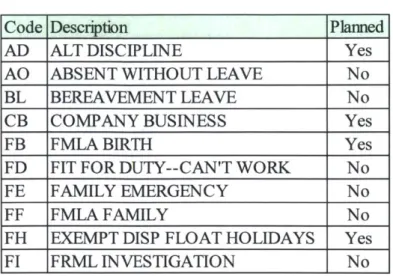
unplanned absences. RailCo uses several description codes in their scheduling operations to
Table 2: Sample absence codes
Code Description Planned
AD ALT DISCIPLINE Yes
AO ABSENT WITHOUT LEAVE No
BL BEREAVEMENT LEAVE No
CB COMPANY BUSINESS Yes
FB FMLA BIRTH Yes
FD FIT FOR DUTY--CAN'T WORK No
FE FAMILY EMERGENCY No
FF FMLA FAMILY No
FH EXEMPT DISP FLOAT HOLIDAYS Yes
FI FRML INVESTIGATION No
Generally, an absence was considered "unplanned" if the scheduler was not aware the employee
would not arrive more than 24 hours in advance and as a result would not have the opportunity to
adjust schedules before the work day started. For series of unplanned absences from one
employee lasting longer than one day, absences were counted as "unplanned" for the first five
consecutive days, and then "planned" for any remaining days. This is because after several days
of consecutive unplanned absences the schedulers would presumably be able to adjust their plans
appropriately to account for the previously "unplanned" absence. By categorizing all absences
by day and shift, we created 4 years x 365 days x 3 shifts = 4,383 day/shift combinations. A
30.0% 25.0% 20.0% 15.0% - -10.0% 5.0% 0.0% 0 1 2 3 4 5 6 7 8 9 10 11 12
Figure 3: Probability Distribution of Absences
3.1 Evaluating Count Data: Introduction
The number of absences that occur on any given shift is categorized as count data, which are
defined as values that are both non-negative and integers. There are several models that can be
employed to evaluate count data; we will discuss the three most common, namely, Binomial,
Poisson, and Negative Binomial.
3.1.1 The Binomial Distribution
The Binomial distribution is the simplest model used to evaluate count data arising from a series
of independent and identical trials that result in either a success or a failure. The probability
mass function for Binomial distributions is given by the equation:
P(X = k) = npk(1 - p)--k (1)
Where n = the number of trials, p = the probability of success of each trial, and k = the number of
successes. As an example of how this would be applied to RailCo, n would represent the number
probability that each employee would be absent from work, and k would represent the number of
employees that were absent on that given day.
Figure 4 shows sample Binomial distributions based on varying values for n and p.
30.0% 25.0% 20.0% 15.0% 10.0% 5.0% 0.0% - n=15, p=.4 -n=15, p=.8 - n=40, p=.4 1 62
1
6 11 16 21 26 31Figure 4: Sample Binomial Distributions based on varying values of n and p
This model is generally used for simple distributions where the probability of success is known.
Because in our research the probability of success is unknown and varies from employee to
employee, this model is not sufficient to analyze the absences that occur at RailCo.
3.1.2 The Poisson Distribution
The Poisson distribution is the most common model used to evaluate count data (Winkelmann,
2008). It is derived from the Binomial distribution as the number of trials increases towards
infinity while holding the probability of success constant. The probability mass function of the
Poisson distribution is:
Where X = E(X) = Var(X) and e = the base of the natural logarithm (2.71828...). Example
probability distributions based on different values of X are shown Figure 5.
Figure 5: Sample Poisson distributions based on varying values of k
The Poisson distribution is most useful if the mean and variance for the data being analyzed are
the same. If the variance of a given set of data is greater than the mean, called over-dispersion,
or smaller than the mean, called under-dispersion, then other models that are more flexible
should be used. The amount of under/over-dispersion is simply the ratio between the variance
and the mean. The distribution of unplanned absences by shift is slightly over-dispersed, so the
Poisson distribution is not the best model for our data, but it will prove useful later in our
analysis.
3.1.3 The Negative Binomial Distribution
The Negative Binomial distribution is a more flexible model than the Poisson distribution and is
a good alternative for modeling count data that is over-dispersed (Winkelmann, 2008) because it
allows the variance to take on a value different from the mean. The probability mass function for
the Negative Binomial distribution is given by the equation:
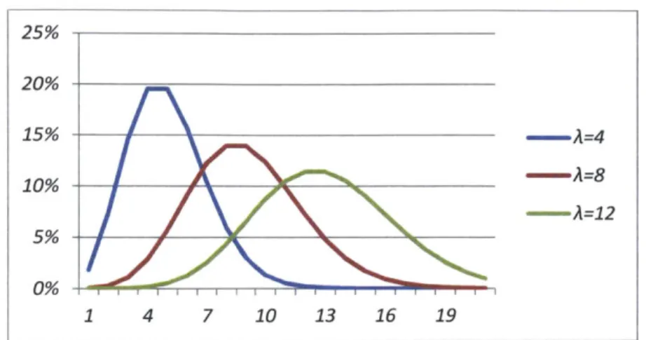
25% 20% 15% -A=4 10% -A=8 -A=12 5%-0% 1 4 7 10 13 1 6 19
(3) P(X = k) = (krl!(1 - p)rpk
Where k = the number of successes, r = the number of failures, and p = the probability of a
success.
The greater flexibility of the Negative Binomial distribution is illustrated in Figure 6, below,
which shows three different distributions based on varying values of r and p.
1 3 5 79 1113151719212325
- r=15, p=.3
- r=10, p=.5
r=5, p=.7
Figure 6: Sample Negative Binomial distributions based on varying values of r and p
We will use the Negative Binomial distribution extensively to model the data we evaluated in
our research. The number of unplanned absences by shift, the number of extra board
qualifications by day/shift, and the number of incumbent qualifications by day/shift can all be
effectively modeled using Negative Binomial distributions.
3.1.4 Goodness of Fit Tests
Goodness of Fit Tests are used to determine how well a distribution approximates the sample
data in question. A common goodness of fit test for the Poisson and Negative Binomial
distributions is the Pearson Chi Square test, which is given by the equation:
16% 14% 12% 10% 8% 6% 4% 2% 0%
2_ e(-fe)2
Xk-P-1= EK f (4)
Where
f
0= the observed frequency, fe = the expected frequency, k = the number of categories, and p = the number of parameters estimated from the data. We will use the Pearson Chi Squaretest to evaluate the goodness of fit for our data to both the Poisson and Negative Binomial
distributions.
3.2 Model Selection
Using the mean and variance as parameters, we fit the distribution of absences to the Poisson
distribution and the Negative Binomial distribution, and tested the degree of fit using the Pearson
Chi Square test. A visual comparison of the distribution of absences by shift to the Poisson and
Negative Binomial distributions is shown in Figure 7.
Poisson Distribution Distribution of Absences - Poisson Distribution 0 1 2 3 4 5 6 7 8 9 10 11 12
Negative Binomial Distribution
0.3 0.25 0.2 0.15 0.1 0.05 0 0 1 2 3 4 5 6 7 8 9 10 1112
Figure 7: Distribution of unplanned absences compared to sample distributions
The Pearson Chi Square goodness of fit tests for our sample data are shown in Table 3.
0.3 0.25 0.2 0.15 0.1 0.05 0 - Distribution of Absences -- Negative Binomial Distribution
Table 3: Goodness of fit tests for absences by shift Negative Binomial
Parameter Estimate Lower 95% Upper 95%
Average k 2.67351 2.6228 2.7249
Overdispersion cy 1.1110 1.0653 1.1599
Chi Square Prob<Chi Square
Chi Square 9.33961 0.7468
Poisson
Parameter Estimate Lower 95% Upper 95%
Average
I
2.67351 2.62541 2.7222Chi Square Prob<Chi Square Chi Square 43.76981<.0001
As seen in Table 3, the chi square value for the Poisson distribution is 43.77. Given that there
are eleven degrees of freedom in this Chi Square test, the resulting probability value is less than
.0001, from which we conclude the data is not from the Poisson distribution. The Chi Square
value for the Negative Binomial distribution is 9.34, producing a probability value of .74, from
which we conclude the Negative Binomial distribution is appropriate to model the number of
unplanned absences.
Fitting the distribution of unplanned absences to distributions of known parameters such as
Poisson and Negative Binomial allows us to use what are known as Generalized Linear Models
to perform regression analysis. Poisson regression and Negative Binomial regression are both
GLMs. Because Poisson regression is the most common GLM for count data, and because it is
robust to over-dispersion and other variances in the data (Winkelmann, 2008), we conducted our
analysis using Poisson regression. Later we will show that the results of using Poisson
regression on our data set are virtually identical to the results of using Negative Binomial
3.3 Generalized Linear Regression Models
Regression analysis is a common tool used to explain the variance in a dependent variable, y, using independent variables, x. The most common form of regression analysis, Ordinary Least
Squares, is not appropriate for our model for a number of reasons. First, OLS assumes that the
residuals are normally distributed, which is not true in our case. Second, OLS is not suitable for
count data because count data must take on positive integer values (Winkelmann, 2008). For this
reason, count data is generally evaluated using GLMs with a link function, such as a logarithm, which forces the variables to be positive. The Poisson Regression Model is an example of a
GLM; a comparison of the Poisson regression to OLS regression is shown below.
Ordinary Least Squares Regression
9 = flo + fi1x1 + fi2X2 + -- + #kXx
Where
y
= the dependent variable, xj= the independent variables, and fli=the effect of the independent variables on the dependent variable.Poisson Regression
Z = exp(fl0 + /31x1 + /32x2 + -- + /3kXk) = efto+#1x1+#2x2+--+#kxk
Where A = the dependent variable, xj= the independent variables, fli=the effect of the
independent variables on the dependent variable, and e= the natural log (2.718...).
The Negative Binomial Regression Model is a GLM like the Poisson Regression Model, and also
GLMs are also different from OLS models in that they have no equation to determine the effect
of independent variables on the dependent variable. Instead, they rely on Maximum Likelihood
Estimations, in which parameters for the model are determined so as to maximize the probability
that the observed data was generated by the given model (Winkelmann, 2008). Maximum
likelihood estimations are computed by mathematical algorithms employed by statistical
software programs.
3.3.1 Goodness of Fit Tests for Generalized Linear Regression Models
One final difference between OLS regression and GLM regression is what methods are used to
measure how well the regression equation fits the actual data, or how effectively the independent
variables predict the value of the dependent variable. OLS regression uses R2 to determine the
level of fit, which is a measure of the percentage of variance in the dependent variable that is
attributable to the variation in the dependent variable. Because GLMs are computed using
Maximum Likelihood Estimators, they do not use the OLS R2 to determine fit, but instead use
other tools that provide a measure of fit that is similar to what R2 is to OLS. The most common
measure of fit for GLMs, used for its robustness, is the McFadden R2 (Veall & Zimmermann,
1996); we will use this measure to assess the fit of our regression models.
3.4 Inputs for Simulation
One purpose of our research was to help RailCo understand the tradeoffs between the number of
extra board employees, the number of qualifications of each employee, the amount of overtime
required, and total labor costs. To understand the relationships between these variables we used
Monte Carlo Simulation. In Monte Carlo Simulation, a number of inputs that each obeys a
running many iterations of this simulation you can gain an understanding of the best solution to
the overall problem (Metropolis, N.; Ulam, S. 1949). In our case with RailCo, the inputs that
obey a probability distribution are the number of absences on a given shift, the number of
qualifications of incumbent employees, and the number of qualifications of extra board
employees. After defining these inputs we assigned dispatchers to positions by using an
optimization solver that was designed for our type of assignment problem. By changing
qualification levels and the number of extra board employees and running simulation iterations
we were able to investigate the impact of varying the number of extra board employees and
qualifications on costs. We will now explain the specific inputs and the optimization portion of
our simulation model.
3.4.1 Distributions of Employee Qualifications
The first step in building a simulation model was to determine the distribution of qualifications
by day/shift of incumbent employees and the distribution of qualifications by day/shift of extra
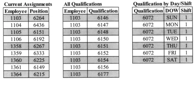
board employees. To do this, we used three relational database tables provided by RailCo, which
are "Current Assignments," "All Qualifications," and "Qualifications by Day/Shift." Sample
Current Assignments Employee Position 1103' 6264 1104 6436 1106 6192 1359 6333 1361 6149 -1364 '6215 All Qualifications Employee Qualification 1103 6147 1103 6150 1103 6152 1103 6156 Qualification by Day/Shift Qualification DOW Shift
6072 MON I
6072 WED I
6072 FRI I
Figure 8: Samples from data tables
The Current Assignments table indicates each employee's number and the position for which he
or she is the incumbent, the All Qualifications table lists every position that each employee is
currently qualified to work on, and the Qualifications by Day/Shift table shows the
corresponding day and shift of each qualification. Some qualifications are used during all seven
days of the week, others are used only for five days, and a few are used on only two days.
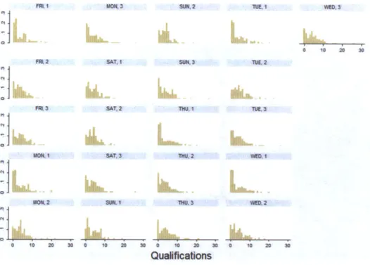
Using the data in from these tables we created a distribution of employee qualifications for each
day/shift combination. The distributions for extra board employees are shown in Figure 9,
SUN 2
h by 0 as
GraPhs by DOW Ond St
SAT, I SUN 3 1W 52 S^ THU,1 1UE 3 Quafifications
Figure 9: Distributions of qualifications for extra board employees
As is evident from Figure 9, each day/shift produces a similar distribution; we fit each of these
distributions to a Negative Binomial distribution using a maximum likelihood estimator and
tested the degree of fit using the Pearson Chi Square test. The statistics that describe each
day/shift distribution and its level of fit to a Negative Binomial distribution is shown in Table 4. SAT, 3 THU, 2 0 a 10 is 11W, 3 z 0 t ... ... ... .... .. .... .... ... ,- - -.... ... . ....
1st Shift
2nd Shift
Table 4: Statistics for distributions of extra board qualifications
Monday Tuesday Wednesday Thursday Friday Saturday Sunday
Average 3.847 3.847 3.847 3.847 3.847 3.647 3.647 Overdispersion 1.431 1.431 1.431 1.431 1.431 1.324 1.324 Chi Square 11.750 11.750 11.750 11.750 11.750 9.045 9.045 P-Value 0.896 0.896 0.896 0.896 0.896 0.959 0.959 Average 3.753 3.753 3.753 3.753 3.753 3.694 3.658 Overdispersion 1.107 1.107 1.107 1.107 1.107 1.122 1.145 Chi Squa 1 14.110 14.110 14.110 14.110 14.110 17.090 16.560 P-value 0.722 0.722 0.722 0.722 0.722 0-517 0.554
We see in Table 4 that the average number of qualifications that each extra board employee has
on Monday first shift is 3.847. The over-dispersion is 1.431, and the Chi Square value for the
Monday first shift distribution is 11.75, which, given sixteen degrees of freedom, produces a
p-value of .896, from which we can conclude that the number of qualifications for extra board
employees on Monday first shift can be appropriately modeled by a Negative Binomial
distribution. Indeed, every day/shift combination produces a p-value above .05, and
consequently can be modeled effectively by a Negative Binomial distribution.
We repeated this process of creating distributions for each day/shift for incumbent employees
with a few minor variations. Unlike extra board employees, who can fill any position on any day without incurring extra cost, incumbent employees can only be scheduled on the unique day and shift to which they are assigned. For this reason, the incumbent's qualifications were only counted on the days and shift when the incumbent was normally scheduled. The distributions for incumbent employee qualifications are shown in Figure 10, below.
Ni
~I
FrA 2
FV 3
MOW. 2
0 10 20 30
MO1 3 SU, 2 1UE.1
SAT. I SAT, 2 SAT, 3 SWI. 3 TNi,2 IMu TUF, 2 TUI,) VKOD WM.2 t20 30 0 1s 30 Qualifications
Figure 10: Distributions of qualifications for incumbent employees
As seen in Figure 10, the distributions of qualifications of incumbent employees by day/shift
have more variation than the distributions of qualifications of extra board employees. We
deducted one from each incumbent employee's count of qualifications and fit the remaining
number to Negative Binomial distributions. We deducted one from every incumbent's count of
qualifications because incumbent employees must have the qualification for the position to
which they are assigned, but we were interested in knowing how many qualifications they had in
addition to their regular assignment. The statistics for incumbent employees and their level of fit
to Negative Binomial distributions is contained in Table 5.
wEo, 3
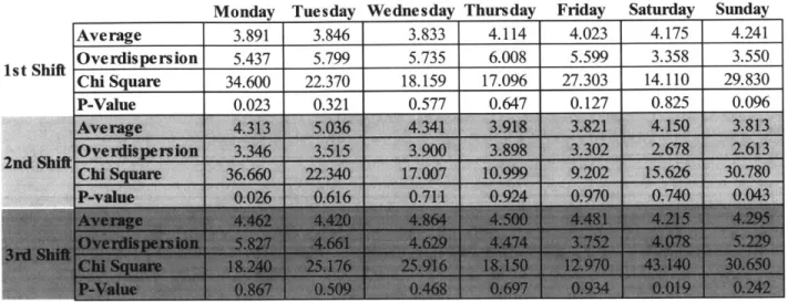
Table 5: Statistics for distributions of incumbent qualifications
Monday Tuesday Wednesday Thursday Friday Saturday Sunday
Average 3.891 3.846 3.833 4.114 4.023 4.175 4.241
Overdispersion 5.437 5.799 5.735 6.008 5.599 3.358 3.550
Chi Square 34.600 22.370 18.159 17.096 27.303 14.110 29.830
0.023 0.321 n r77 I 6d7 I 177 I ) R7i5 0096
Table 5 shows only four out of twenty-one day/shift p-values (Monday first, Monday second,
and Saturday third, and Sunday second) that are below .05 when fit to Negative Binomial
distributions. Friday third shift has the highest p-value of .934. The sum of p-values for Friday
third shift is .934+.968=1.902, which is the highest sum for any day/shift combination; we
selected Friday third shift for our simulation for this reason.
3.5 Optimization
We will now explain the optimization portion of our simulation model. To find a solution that
minimizes cost we used a pre-programmed optimization solver that was designed for assignment
problems like ours. This optimization problem is written mathematically as:
(5) Mm ZN+E+l ein =1E+ Z5Y~='J 1
1 Cii Subject to: xij 1,< ZN+E+lXj = 1 i N + E (6) (7) j:5 N 1st Shift P-Value
xij 5 ati (8)
a1, xu E (0,1) (9)
Where cij is the cost of assigning person i to jobj; xij = 1 if person i is assigned to job
j
at acertain time and 0 otherwise; aij = 1 if person i is qualified for job
j
and 0 otherwise. N is both the number of positions on any given day and shift, and the number of incumbent employees; E isthe number of extra board dispatchers.
In solving this problem, we generated two matrices, the first of which is shown in Figure 11.
Position 1 2 3 4... N S1 o 2 . E 3 4 .a . N 1 0 1 1 --- 1 N+1 -Mi N+2 0 II N+E
Employee from Home N+E+1
Figure 11: Qualification Matrix
In Figure 11, the 1's represent the qualifications of each employee. The horizontal numbers from 1 to N represent positions and the vertical numbers, going from 1 to N, represent individual
employees. For example, incumbent employee 2 is qualified for position 2 but not qualified for
1 1 0 0 ... 0
0 1 0 1 ... 1
O i 1 0... 0
position 1. The diagonal of the matrix is filled with 1's, which represents the incumbent
employees in their regular positions.
Rows from N+1 to N+E represent the extra board employees; the 1's and O's in these rows also
represent qualifications. For example, extra board employee N+2 is qualified on position 3 and 4,
but not qualified on positions 1 and 2, etc.
The last row represents the pool of dispatchers that can be called from home and paid overtime
to work in any position. These are all 1's because we are assuming any position on any given day
and shift can be filled by an employee that can be called from home.
The second matrix is the cost matrix, shown in Figure 12.
03 E U.' .0 E 0 Ei e Employee from Home
1 2 3 4 N N+1 N+2 N+E N+E+1 Position 1 2 3 4 .... N
Figure 12: Cost Matrix
The matrix in Figure 12 has an identical structure to Figure 11; the horizontal numbers from 1 to
N represent positions and the vertical numbers from 1 to N represent employees. Each cell in this 0 0.5 X X -. X
X 0 X 0.5 ... 0.5
X X 0 X ... X
matrix represents the cost of assigning the employee of that row to the position of that column.
An "X" in a cell indicates that employee is not qualified for that position and cannot be assigned
there. For example, if employee 2 is assigned to position 4, the overtime cost will be 0.5, but if
that employee is assigned to position 2, which is her scheduled position, there is no extra cost;
employee 4 cannot be assigned to position 1 or 3, and therefore the corresponding cells are filled
with X's. In the actual simulation program, cells with X's will be assigned a large number that
will force the optimization software not to pick any of those cells.
In Figure 12, the rows from N+1 to N+E represent extra board employees, and according to the
company policy, there is no overtime cost to assign an extra board employee to a position that
he/she is qualified for, and so the cells in these rows will be either X or 0.
The last row in Figure 12 represents the pool of dispatchers that can be called from home and
paid overtime to work in any position. According to RailCo policy, employees that are called
from home must be paid time and a half per day.
Now that we have established a matrix of qualifications and a matrix of costs, we can use the
solver to find the optimal solution. As the solver is employed it will generate a third matrix that
represents the assignments that lead to a minimum cost. An example of what this will look like
S1 0 2 4. E 3 C 4 E Position 1 2 3 4... N 1 0 0 ... 0 0 0 0 0 --- 0 0 0 1 0 ... 0 0 0 0 0 ... 0 . N 0 0... I N+1 i N+2 wU N+E Employee from Home N+E+1
Figure 13: Solution Matrix
In this solution matrix, 1's represent the assignment of employees to positions. For example, positions 1 and 3 are filled by the incumbent employee, position 2 is filled by extra board
employee N+1, and position 4 is filled by an employee called from home. The sum of the values in each column must be 1, meaning that every position must be filled by exactly one person, and the sum of each row that represents incumbent employees and extra-board employees must be 1 or 0, indicating that each person can only be assigned to a maximum of one position. The last row, which represents employees called from home, can have a sum of zero, one, or any number greater than one up to N, meaning that any number of employees could be called from home to fill vacant positions.
3.6 Simulation
We will now give a summary of the simulation using all the parameters described above. The steps to the final simulation are as follows:
1. Generate a qualification matrix with N+ E+ 1 rows and N columns, each cell having
values of O's or 1's, with 1 representing the corresponding employee qualification and 0
signifying that employee is not qualified on that position. Each incumbent employee has
the qualification for his/her regular position plus some number of qualifications that is
generated using the parameters of the Negative Binomial distribution for any chosen
day/shift that is shown in Table 5. Each extra board employee is assigned some number
of qualifications that is generated using the parameters of the Negative Binomial
distribution for any chosen day/shift shown in Table 4. For both incumbent and extra
board employees, the positions for which they receive qualifications are randomly
distributed, with each position being equally likely. The last row of the assignment
matrix is filled with 1's because any position can be filled by someone called from home.
2. Generate a cost matrix of identical size to the qualification matrix, in which each entry in
the matrix represents the cost associated with that employee working in that position.
3. Generate a certain number of absences based on the parameters of the Negative Binomial
distribution for unplanned absences that is shown in Table 3, and randomly assign those
absences to incumbent and extra board employees, with every employee having an
equally likely chance of being absent. To indicate an absence in our simulation we
included a constraint in the matrix, namely, that the sum of the row for an absent
employee must be zero.
4. Use a linear program solver to make assignments for all positions in a way that
minimizes the total cost that results from the number of slides that occurred and the
5. Run 10,000 iterations of this simulation in which each iteration generates a new
qualification matrix, a new set of absences, a new solution matrix, and a resulting total
cost. This simulation will produce an expected cost given the pre-determined number of
extra board employees and the pre-determined average number of qualifications.
6. Adjust the number of extra-board employees and the average number of the qualifications
and repeat the simulation starting with step 1.
This simulation could be used to simulate any combination of day/shift, number of extra board
employees, and average number of qualifications. We chose to model Friday third shift in our
analysis; the corresponding "N" for our model was eighty-five, as seen in Table 6, which shows
the number of regular positions that must be filled for each day and shift.
Table 6: Number of positions for each day and shift
M ON WVED FRI SUN
Shiftl 1
2
I3
112 131
3
11
2
13
Number of Positions ,96 90 85 96- 9085 99085 88875
In our simulations we varied the number of extra board employees from zero to twenty, and used
eight different qualification levels for extra board employees. The average qualification level of
incumbent employees was not varied during our simulations. The average number of
qualifications of extra board employees and incumbent employees is shown in Table 7.
Table 7: Mean and standard deviation of each employee type
Mean Standard Deviation
Normal Extra Normal Extra
The average number of qualifications of extra board employees is 11.22, while on each day and
shift their average number of qualifications is 3.6756. Therefore, if every extra board employee
receives an average of one more qualification, the average number of qualifications per shift
increases by 0.327, which is 11.22 divided by 3.6756. In our simulation we will add or deduct a
multiple of 0.327 to increase or decrease of the average level of qualifications per employee.
Table 8 shows the eight qualification levels we used in our simulation and the overall
qualification levels they represent.
Table 8: Average qualifications per employee
Average Qualifications Average Qualifications per employee per employee per shift
9.22 2.852
11.22 3.506
13.22 4.160
15.22 4.814
4 Data Analysis: Regression
Our analysis aimed to construct a model that would allow RailCo to predict the number of
absences that would occur on any given shift. To test whether such a model was possible, we
identified several factors that might influence the number of absences on a company-wide scale.
We compiled this list of possible factors after considering previous work in the literature and
suggestions by RailCo scheduling management. Table 9 shows the list of factors considered in
Table 9: Possible factors that influence unplanned absences
Day of the Month
Shift
Football Games
Snow Storms
We evaluated these parameters using backward stepwise regression, in which all the parameters
were included in the model, and then insignificant parameters were eliminated one at a time until
only statistically significant factors remained. The null hypothesis in this case is that the effect of
the parameters is zero, and the alternative hypothesis is that the effect is non-zero. Parameters
with p-values above .05 were not considered to provide enough evidence to reject the null
hypothesis (i.e., they were not considered to contribute significantly to unplanned absences).
These factors included day of the month, day of the week, planned absences, hunting season, and
football games. The parameters that produced p-values less than .05 were assumed to exhibit
evidence sufficient to reject the null hypothesis of non-significance. The parameters considered
significant included shift, month, selected holidays, and snow storms. The next section describes
how we constructed and evaluated the parameters contained in the model. We will conclude our
data analysis by examining two trends that are apparent over the four year period that we
evaluated, which are the number of absences by year and the number of absences attributable to
4.1 Statistically Significant Parameters
The four parameters that produced p-values of less than .05 were month, shift, holidays, and
snowstorms.
4.1.1 Month
From our regression analysis it is apparent that month does have an impact on the number of
unplanned absences at RailCo. July has the lowest average of unplanned absences so it was
taken as the base value to which the other months were compared. Table 10 gives a breakdown
of each month and its respective p-value.
Table 10: Regression statistics for month
Month Coef. Actual Effect Std. Err. z P>z Lower 95% int Upper 95% int
feb 0.251001 0.671053 0.050121 5.01 <.0001 0.152766 0.349235
apr 0.245267 0.655723 0.047538 5.16 <.0001 0.152094 0.338440 jun 0.092801 0.248105 0.047902 1.94 0.053 -0.001085 0.186687
sep 0.003406 0.009106 0.049479 0.07 0.945 -0.093571 0.100383
nov 0.043576 0.116500 0.049186 0.89 0.376 -0.052827 0.139978
As seen in Table 10, January, February, March, April, October and December all display
p-values below the .05 level, from which we conclude that these months do have a non-zero effect
on unplanned absences. May, June, August, September, and November do not produce values
that are statistically different from July, the lowest month. There may be many factors that
in sickness among the workforce, the number of allotted planned absences, or other idiosyncratic
factors not evaluated in our model.
4.1.2 Shift
Shift also has a non-zero effect on the number of unplanned absences that occurred over the four
year period. RailCo can expect a slightly higher number of absences on second and third shifts
as compared to first shifts. These findings are in Table 11. It makes intuitive sense that third
shift would have the highest number of unplanned absences given that it starts sometime between
the hours of 9:00 PM and 4:59 AM.
Table 11: Regression statistics for shift
Shift Coef. Actual Effect Std. Err. z P>z Lower 95% int Upper 95% int
shift2l 0.066634' 01S A
X264
0 .4 OQ~ O12~ 0.83shift3 0.101265 0.270733 0.023696 4.27 <.0001 0.054822 0.147709 A
4.1.3 Holidays
The Holidays we evaluated in our regression model were selected based on a 2010 study
conducted by Worldatwork. This study found that the average number of paid holidays in the
United States is 8.7. This study also presented a list of the most common paid holidays, from
Table 12: Nine most common paid Holidays
New Years Day Labor Day
hIdependence Day Day after Thanksgiv n Presidents Day
For New Year's Day we combined the third shift of New Year's Eve because it technically runs
into New Year's Day. In addition to these nine paid holidays, we created one other holiday
parameter called "Federal Holidays," which is a combination of Martin Luther King Jr. Day,
Columbus Day, and Veterans Day. These three days are Federal Holidays but were not included
in the top nine Holidays cited in the Worldatwork study.
The results, shown below in Table 13, indicate that the most popular Holidays have the
somewhat surprising effect of lowering the number of absences for any given day. This is true
for New Year's, President's Day, Independence Day, Thanksgiving, Christmas Eve, and
Christmas. The remaining holidays, Labor Day, Memorial Day, the Friday after Thanksgiving,
Table 13: Regression statistics for Holidays
Holiday Coef. Actual Effect Std. Err. z P>z Lower 95% int U er 95% int
presidents -0.420272 -1.122878 0.206649 -2.03 0.042 -0.825297 -0.015248
independence -0.916658 -2.448851 0.303559 -3.02 0.003 -1.511622 -0.321694
thanksgiving -1.171696 -3.104133 0.335387 -3.49 <.0001 -1.829043 -0.514350
christmaseve -0.841878 -2.248154 0.260941 -3.23 0.001 -1.353313 -0.330443
federal 0.010323 0.000000 0.101771 0.10 0.919 -0.189144 0.209790
Based on the values in Table 13, RailCo can expect two to three fewer absences on shifts on
popular holidays. While these results may be somewhat counter-intuitive, it seems reasonable
that the stigma of calling in sick on a holiday is great enough to give dispatchers extra motivation
to arrive at work. It may also be that employees are extra-motivated to come to work on
holidays because of the negative effect it has on other employees that are forced to fill in for the
absent employee.
4.1.4 Snowstorms
One final parameter that shows a high degree of significance in contributing to unplanned
absences is snow storms. Twenty shifts included in our model were noted as having had
significant snowstorms; data on snow storm dates and severity was taken from list of snow
events compiled by the National Weather Service for the local area. The effect of snowstorms
on absences is shown in Table 14. According to our analysis, RailCo can expect an extra 2.16
absences on shifts that have snowstorms.
Table 14: Regression statistics for snowstorms
Event Coef. Actual Effect Std. Err. z P>z Lower 95% int Upper 95% int
This finding is not particularly helpful in predicting future absences in the long range because it
is difficult to accurately forecast the weather, but it may be helpful for RailCo in their short term
planning.
4.1.5 Planned Absences
There were three types of planned absences included in this parameter: scheduled vacation, float
vacation, and personal days. These planned absences did not have a significant effect on
unplanned absences by themselves, as seen in Table 15. However, removing them from the
model it has the effect of lowering the statistical significance of other parameters and reducing
the overall predictive capability of the model. This effect of parameters being influenced by
each other is known as co-linearity. For this reason, it is useful to consider planned absences as a
significant factor even though their p-value, at .106, is slightly higher than .05.
Table 15: Regression statistics for planned absences
Parameter Coef. Std. Err. z P>z Lower 95% int Upper 95% int
4.2 Statistically Insignificant Factors
There are a number of parameters that do not give us enough evidence to conclude that their
effect on absences is not zero. These include football games, day of the month, and day of the
week. We will now discuss these parameters in detail.
4.2.1 Hunting Season
Hunting season in the local area, begins every year on the first Sunday in November and ends on
hunting season" parameter to the last two days of hunting season each year. As seen in Table 16,
the beginning of hunting season was found to be insignificant regarding absences, with a p-value
of .493, and the end of hunting season was insignificant with a p-value of .08. The data do not
provide sufficient evidence to conclude that the effect of hunting season in November and
December is greater than zero.
Table 16: Regression statistics for hunting season
Parameter Coef. Actual Effect Std. Err. z P>z Lower 95%int Upper95% int Beg Hunt Season -0.0965931 0.0(d0 0L4t805 -069 0493 4372566 .179380
End Hunt Season 0.217245 0.580145 0.124163 1.75 0.080 -0.026110 0.460601
4.2.2 Football Games
We evaluated two types of football games: the Super Bowl and regular season NFL games. The
"NFL" parameter in Table 17 includes all dates on which NFL games were played, and the
"Super Bowl" parameter includes all shifts of the days on which the Super Bowl was played.
From the p-values of .702 and .284 for NFL and Super Bowl, respectively, there is insufficient
evidence to conclude that NFL football games or the Super Bowl affect unplanned absences.
Table 17: Regression statistics for football games
Parameter Coef. Std. Err. z P>z Lower 95% int Upper 95% int
NFL AW IB4 4. 04 T 0Z 47~ ~~3
Super Bowl -0.19899 0.18556 -1.07 0.284 -0.562688 0.164712
4.2.3 Day of the week and Day of the Month
The data for day of the month is shown in Table 18. The first day of each month was used as the
base number to which all the other days of the month were compared. There are a few days of
month to be considered, we used a .01 test of probability for this parameter. At this level of significance there were no days of the month that showed significance.
Table 18: Regression statistics for days of the month
DaV Coef. Std. Err. z P>z Lower 95%int Upperin5%tnt
3 -0.12347 0.07218 -1.71 0.087 -0.264952 0.018007
5 -0.09289 0.07223 -1.29 0.198 -0.234458 0.048668
__OWA5 04M36 -O2021 =-~ot
7 -0.04398 0.07161 -0.61 0.539 -0.184337 0.096377 8 0~~i1-.7i 0.4 0~5 ~ 7~c .10737 9 -0.00183 0.07017 -0.03 0.979 -0.139356 0.135698 11 -0.09151 0.07222 -1.27 0.205 -0.233062 0.050052 1 -0. O.0746 .7w 0073 -Z71$36 0.QZ22O3 13 -0.12053 0.07256 -1.66 0.097 -0.262744 0.021689 15 -0.14450 0.07323 -1.97 0.048 -0.288020 -0.000977 17 -0.09610 0.07218 -1.33 0.183 -0.237561 0.045369 $ -0.06988 007167 -029 ______ 0.070605 19 -0.12545 0.07265 -1.73 0.084 -0.267853 0.016944 21 -0.08126 0.07183 -1.13 0.258 -0.222041 0.059530 23 -0.09835 0.07206 -1.36 0.172 -0.239597 0.042891 25 -0.08073 0.07422 -1.09 0.277 -0.226193 0.064734 27 -0.14174 0.07316 -1.94 0.053 -0.285130 0.001650 29 -0.08360 0.07325 -1.14 0.254 -0.227158 0.059957 31 -0.03626 0.08357 -0.43 0.664 -0.200044 0.127532
Day of the week also showed no statistical significance when evaluated at the .05 level. Table