HAL Id: hal-00180601
https://hal.archives-ouvertes.fr/hal-00180601
Submitted on 19 Oct 2007
HAL is a multi-disciplinary open access
archive for the deposit and dissemination of
sci-entific research documents, whether they are
pub-lished or not. The documents may come from
teaching and research institutions in France or
abroad, or from public or private research centers.
L’archive ouverte pluridisciplinaire HAL, est
destinée au dépôt et à la diffusion de documents
scientifiques de niveau recherche, publiés ou non,
émanant des établissements d’enseignement et de
recherche français ou étrangers, des laboratoires
publics ou privés.
A Parameterized Algorithm for Exploring Concept
Lattices
Peggy Cellier, Sébastien Ferré, Olivier Ridoux, Mireille Ducassé
To cite this version:
Peggy Cellier, Sébastien Ferré, Olivier Ridoux, Mireille Ducassé. A Parameterized Algorithm for
Exploring Concept Lattices. Int. Conf. Formal Concept Analysis, Feb 2007, France. pp.114–129.
�hal-00180601�
A Parameterized Algorithm for Exploring
Concept Lattices
Peggy Cellier1, S´ebastien Ferr´e1, Olivier Ridoux1 and Mireille Ducass´e2
1IRISA/University of Rennes 1 and2IRISA/INSA,
Campus universitaire de Beaulieu, 35042 Rennes, France [email protected], http://www.irisa.fr/LIS/
Abstract. Formal Concept Analysis (FCA) is a natural framework for learning from positive and negative examples. Indeed, learning from ex-amples results in sets of frequent concepts whose extent contains only these examples. In terms of association rules, the above learning strat-egy can be seen as searching the premises of exact rules where the conse-quence is fixed. In its most classical setting, FCA considers attributes as a non-ordered set. When attributes of the context are ordered, Conceptual Scaling allows the related taxonomy to be taken into account by produc-ing a context completed with all attributes deduced from the taxonomy. The drawback, however, is that concept intents contain redundant in-formation. In this article, we propose a parameterized generalization of a previously proposed algorithm, in order to learn rules in the presence of a taxonomy. The taxonomy is taken into account during the compu-tation so as to remove all redundancies from intents. Simply changing one component, this parameterized algorithm can compute various kinds of concept-based rules. We present instantiations of the parameterized algorithm for learning positive and negative rules.
1
Introduction
Learning from examples is a fruitful approach when it is not possible to a priori design a model. It has been mainly tried for classification purposes [Mit97]. Classes are represented by examples and counter-examples, and a formal model of the classes is learned by a machine.
Formal Concept Analysis (FCA) [GW99] is a natural framework for learning from positive and negative examples [Kuz04]. Indeed, learning from positive examples (respectively negative examples) results in sets of frequent concepts with respect to a minimal support, whose extent contains only positive examples (respectively negative examples). In terms of association rules [AIS93,AS94], the above learning strategy can be seen as searching the premises of exact rules where the consequence is fixed. When augmented with statistical indicators like confidence and support it is possible to extract various kinds of concept-based rules taking into account exceptions [PBTL99,Zak04].
The input of FCA is a formal context that relates objects and attributes. FCA considers attributes as a non-ordered set. When attributes of the context
are ordered, Conceptual Scaling [GW99] allows the attribute taxonomy to be taken into account by producing a context completed with all attributes deduced from the taxonomy. The drawback is that concept intents contain redundant information. In a previous work [CFRD06], we proposed an algorithm based on Bordat’s algorithm [Bor86] to find frequent concepts in a context with taxonomy. In that algorithm, the taxonomy is taken into account during the computation so as to remove all redundancies from intents.
There are several kinds of association rules, and several related issues: e.g. find all association rules with respect to some criteria, compute all association rules with a given conclusion or premise. We propose a generic algorithm to address the above issues. It is a parameterized generalization of our previous algorithm. It learns rules and is able to benefit from the presence of a taxon-omy. The advantage of taking a taxonomy into account is to reduce the size of the results. For example, the attributes of contexts about Living Things are intrinsically ordered 1. For a target such as “suckling”, a rule such as “Living Things”∧ “Animalia” ∧ “Chordata” ∧ “Vertebrata” ∧ “Mammalia” → “suck-ling” is less relevant than the equivalent rule “Mammalia”→ “suckling” where elements redundant with respect to the taxonomy have been eliminated. The presented algorithm can compute various kinds of concept-based rules by simply changing one component. We present two instantiations which find positive and negative rules. Positive rules predict some given target (e.g. predict a mushroom as poisonous), while negative rules predict its opposite (e.g. edible).
The contributions of this article are twofold. Firstly, it formally defines FCA with taxonomy (FCA-Tax) using the Logical Concept Analysis (LCA) frame-work [FR04], where the taxonomy is taken into account as a specific logic. Sec-ondly, it specifies a generic algorithm which facilitates the exploration of frequent concepts in a context with taxonomy. Quantitative experiments show that taking a taxonomy into account does not introduce slowdowns. Furthermore, the prun-ing implemented by our algorithm related to the taxonomy can often improve efficiency.
In the following, Section 2 formally defines FCA with taxonomy (FCA-Tax). Section 3 presents the generalization of the algorithm described in [CFRD06] to filter frequent concepts in a formal context with taxonomy. Section 4 shows how to instantiate the algorithm to learn different kind rules. Section 5 discusses experimental results.
2
A Logical Framework for FCA with Taxonomy
In this section, we formally describe Formal Concept Analysis with Taxonomy (FCA-Tax) using the Logical Concept Analysis (LCA [FR04]) framework. We first present an example of context with taxonomy. Then we briefly introduce LCA, concept-based rules, and we instanciate LCA to FCA-Tax. A taxonomy describes how the attributes of the context are ordered and thus a taxonomy is a kind of logic where the subsumption relation represents this order relation.
2.1 Example of Context with a Taxonomy
Pacific Southwest Southe ast
Region8 Hawai Washington Arizona Michigan Mississipi Florida Utah Alaska Or egon
California Nevada Endanger ed Thr eatene d Accipitridae • • Alcedinidae • • Alcidae • • • • Anatidae • • Cathartide • • Charadriidae • • • • • Corvidae • • Drepanidinae • • Emberizidae • • Gruidae • • • Icteridae • • Muscicapidae • • Strigidae • • • • • • Tyrannidae • • • • • Vireonidae • •
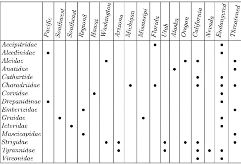
Table 1.Context of threatened or endangered bird families in the USA
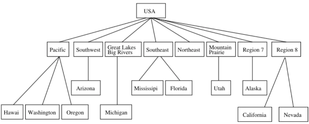
The context given Table 1 represents the observations of threatened and endangered bird families. Data come from the web site of USFWS2 (U.S Fish and Wildlife Service). The objects are bird families and each family is described by a set of states and regions where specimens have been observed and by a status: threatened or endangered . Note that in this context objects are elements of what could be a taxonomy in another context. Figure 1 shows the taxonomy of states and regions of USA.
The context given in Table 1 is the straightforward transcription of the infor-mation found on the USFWS site. Note that it is not completed with respect to FCA. For example object Accipitridae which has in its description the attribute Florida has not the attribute Southeast. The information that an object has the attribute Florida implies that it has the attribute Southeast is implicitly given by the taxonomy. We have observed that this situation is quite common. 2.2 Logical Concept Analysis (LCA)
In LCA the description of an object is a logical formula instead of a set of attributes as in FCA.
USA
Southeast
Mississipi Florida Northeast Great Lakes
Big Rivers MountainPrairie
Utah Arizona Southwest Region 7 Alaska Region 8 California Nevada Pacific Michigan Oregon Washington Hawai
Fig. 1.Taxonomy of USA states and regions.
Definition 1 (logical context). A logical context is a triple (O, L, d) where O is a set of objects, L is a logic (e.g. proposition calculus) and d is a mapping fromO to L that describes each object by a formula.
Definition 2 (logic). A logic is a 6-tuple L = (L, v, u, t, >, ⊥) where – L is the language of formulas,
– v is the subsumption relation,
– u and t are respectively conjunction and disjunction, – > and ⊥ are respectively tautology and contradiction.
Definition 3 defines the logical versions of extent and intent. The extent of a logical formula f is the set of objects inO whose description is subsumed by f. The intent of a set of objects O is the most precise formula that subsumes all descriptions of objects in O. Definition 4 gives the definition of a logical concept. Definition 3 (extent, intent). Let K = (O, L, d) be a logical context. The definition of extent and intent are:
– ∀f ∈ L ext(f) = {o ∈ O | d(o) v f } – ∀O ⊆ O int(O) =Fo∈O d(o)
Definition 4 (logical concept). LetK = (O, L, d) be a logical context. A log-ical concept is a pair c = (O, f ) where O⊆ O, and f ∈ L, such that int(O) ≡ f and ext(f ) = O. O is called the extent of the concept c, i.e. extc, and f is called its intent, i.e. intc.
The set of all logical concepts is ordered and forms a lattice: let c and c0 be two concepts, c≤ c0
iff extc⊆ extc0. Note also that c≤ c0 iff intcv intc0. c is called
a subconcept of c0.
The fact that the definition of a logic is left so abstract makes it possible to accommodate non-standard types of logics. For example, attributes can be valued (e.g., integer intervals, string patterns), and each domain of value can be defined as a logic. The subsumption relation allows to order the terms of a taxonomy.
2.3 Concept-Based Rules
Definition 5 (concept-based rules). Concept-based rules consider a target W ∈ L such that W is a logical formula which represents a set of objects, ext(W ), that are positive (respectively negative) examples. Concept-based rules have the form X → W , where X is the intent of a concept. A rule can have exceptions. These exceptions are measured with statistical indicators like support and confidence, defined below.
Neither FCA nor LCA take into account the frequency of the concepts they define. An almost empty concept is as interesting as a large one. Learning strat-egy, however, is based on the generalization of frequent patterns. Thus, statisti-cal indicators must be added to concept analysis. There exists several statististatisti-cal measures like support, confidence, lift and conviction [BMUT97]. In the following, support and confidence are used to measure the relevance of the rules, because they are the most widespread. However, the algorithm presented in this article does not depend on this choice.
Definition 6 (support). The support of a formula X is the number of objects described by that formula. It is defined as:
sup(X) =kext(X)k wherekY k denotes the cardinal of a set Y.
The support of a rule is the number of objects described by both X and W . It is defined as:
sup(X → W ) = kext(X) ∩ ext(W )k
Definition 7 (confidence). The confidence of a rule X → W describes the probability for objects that are described by X to be also described by W . It is defined as:
conf (X→ W ) = kext(X) ∩ ext(W )k kext(X)k
The support applies as well to concepts as to rules. In the case of concept it introduces the notion of frequent concept as formalized by Definition 8.
Definition 8 (frequent concept). A concept is called frequent with respect to a min sup threshold if sup(intc) is greater than min sup.
2.4 Formal Concept Analysis with Taxonomy
FCA-Tax is more general than FCA because the attributes of the context are ordered. It can be formalized in LCA.
Definition 9 (taxonomy). A taxonomy is a partially ordered set of terms T AX =< T,≤ >
where T is the set of terms and≤ is the partial ordering. Let x and y be attributes in T , x≤ y means that y is more general than x.
Example 1. In Figure 1, Hawai ≤ Pacific ≤ USA.
Definition 10 (predecessors, successors, Mintax). Let T AX =< T,≤ > be a taxonomy and X in T be a set of terms.
The predecessors of X in the taxonomy T AX are denoted by ↑tax(X) ={ t ∈ T | ∃x ∈ X : x ≤ t } The successors of X in the taxonomy T AX are denoted by
succtax(X) ={ t ∈ T | ∃x ∈ X : x > t ∧ (6 ∃t0 ∈ T : x > t0> t)}
The successors represented by succtax(X) are immediate ones only. succ+tax(X) is the transitive closure of succtax(X), i.e. all successors of X in the taxonomy. M intax(X) is the set of minimal elements of X with respect to T AX.
M intax(X) ={ t ∈ X | 6 ∃x ∈ X : x < t }
In fact, M intax(X) is X minus its elements that are redundant with respect to T AX.
Example 2. On the context of Table 1, with the taxonomy of Figure 1, examples of predecessors, successors and M intaxare as follows:
– ↑tax({Mississipi, Arizona}) = {Mississipi, Southeast, Arizona, Southwest, USA}
– succtax({USA}) = {Pacific, Southeast, GreatLakes/BigRivers, Southwest, Northeast, Mountains/Prairie, Region7 , Region8} – M intax({Florida, Southeast, USA}) = {Florida}
Definition 11 (Ltax). Let T AX =< T,≤ > be a taxonomy. Ltax= (Ltax,vtax ,utax,ttax,>tax,⊥tax) is the logic of FCA-Tax, related to T AX:
– Ltax = 2T where T is the set of terms,
– vtax such that Xv Y iff ↑tax(X) ⊇ ↑tax(Y ), – utax is∪tax such that X ∪taxY = M intax(X∪ Y ),
– ttax is∩tax such that X ∩taxY = M intax(↑tax(X)∩ ↑tax(Y )), – >tax={x ∈ T | ext({x}) = O}
L= {{Hawai }, {Oregon}, {Pacific}, {Southwest }, ..., {USA}, (1) {Hawai, Southwest }, ...}
{Michigan, Florida} v {Michigan, Southeast } (2) {Michigan, Southeast } u {Florida} = {Michigan, Florida} (3) {Mississipi } t {Florida} = {Southeast } (4) > = {USA} (5) ⊥ = {Hawai, Washington, Oregon, Arizona, Michigan, Mississipi, (6)
Florida, Utah, Alaska, California, Nevada}
Fig. 2.Examples of operations on the attributes of the taxonomy of Figure 1.
u and t follow the usage of description logics, where u (resp. t) corresponds to intersection (resp. union) over sets of objects.
Example 3. Figure 2 shows examples of operations on the context of bird families. The language, L is the powerset of attributes (1). Florida implies Southeast in the taxonomy, thus all bird families observed in Michigan and Florida can also be said to have been observed in Michigan and Southeast (2). To be observed in Florida is an information more precise than to be observed in Southeast, thus only the attribute Florida is kept in (3). The fact that birds are observed in Michigan or Florida can be generalized by birds which are observed in Southeast (4). The top concept contains only one attribute USA (5), and the bottom concept all minimal attributes (6).
All notions defined in LCA apply in FCA-Tax, in particular extent, intent, and concept lattice. Note that the intents of two ordered concepts c < c0
differ because one or more attributes are added in int(c), or because an attribute of int(c0) is replaced in int(c) by a more specific attribute in the taxonomy, or a combination of both. FCA-Tax differs from FCA in that the intents of concepts in FCA-Tax are without redundancy (see the use of M intax in the definition oft).
Example 4. ext(Oregon, Calif ornia) ={Alcidae, Strigidae} int(Alcedinidae, Corvidae) ={P acific, Endangered} sup(Oregon, Calif ornia→ T hreatened) = 2
conf (Calif ornia→ T hreatened) = 0.5
Note in the example about the computation of intent that Corvidae has not explicitly the property P acif ic but the property Hawai. But in the taxonomy the property Hawai implies the property P acif ic.
3
A Parameterized Algorithm for Finding Concept-Based
Rules
In a previous article [CFRD06] we described an algorithm for finding frequent concepts in a context with taxonomy. The algorithm is a variant of Bordat’s algorithm [Bor86] which takes care of the taxonomy for avoiding redundant intents. In this section, a generalization of this algorithm is described in order to search concept-based rules. In a first step, the relation between frequent concepts and rules is presented. In a second step, the parameterized algorithm with this filter function is described.
3.1 From Frequent Concepts to Rules
Relevant rules are rules that are frequently observed. In the general case, see for example [PBTL99], all frequent rules are searched, without any constraint on the premises and conclusions. However, in the learning case, either the premise or the conclusion is fixed by the learning target. So, one searches for frequent rules where conclusions or premises match the target. For instance, learning sufficient conditions for a target W is to search frequent rules like X→ W . For example, in a context describing mushrooms it can be relevant to search properties implying that a mushroom is poisonous, i.e. X → poisonous.
As explained in Section 2, the frequency of a rule is evaluated by a statis-tical measure: the support. A rule cannot be more frequent than its premise or its conclusion. Indeed, let c be a concept then sup(intc)≥ sup(intc∪ W ) = sup(intc → W ). This implies that only the intents of frequent concepts are good candidates to be the premises of the searched rules. Therefore, in order to learn rules, the frequent concepts that are computed by the algorithm pre-sented in [CFRD06] need to be filtered. Only most frequent concepts that form relevant rules with respect to statistical measures are kept. Some statistical mea-sures like the support, are monotonous. For instance, given two concepts c and c0, c < c0
⇒ sup(c) < sup(c0) holds. It means that if the support of a concept c is lower than min sup, all subconcepts of c have a support lower than min sup. Thus, it is not relevant to explore subconcepts of c.
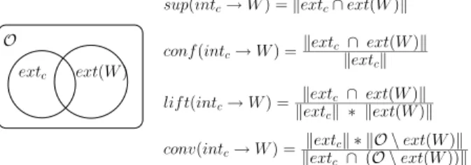
A filter function, called FILTER, is defined in order to take into account these observations. FILTER takes two parameters, two sets of objects: extcand ext(W ). These two parameters are sufficient to compute all statistical measures like support, confidence, lift and conviction as it is illustrated in Figure 3. Using extc and ext(W ), we can compute extc∪ ext(W ), extc∩ ext(W ), and all com-plements likeO \ extc,O \ (extc∪ ext(W )). FILTER(extc, ext(W )) returns two booleans: KEEP and CONTINUE. KEEP tells whether intc→ W is a rele-vant rule with respect to statistical measures. CONTINUE allows monotonous properties to be considered. Indeed, CONTINUE tells whether there may be some subconcept c0 of c such that int
c0 → W is a relevant rule. Thus FILTER
gives four possibilities: 1) keep the current concept and explore subconcepts, 2) keep the current concept and do not explore subconcepts, 3) do not keep the current concept and explore subconcepts, 4) do not keep the current concept
extc O ext(W ) conf(intc→ W ) = kextc∩ ext(W )k kextck conv(intc→ W ) = kextck ∗ kO \ ext(W )k kextc∩ (O \ ext(W ))k
sup(intc→ W ) = kextc∩ ext(W )k
lif t(intc→ W ) =
kextc ∩ ext(W )k
kextck ∗ kext(W )k
Fig. 3.Computing measures using the extents of a concept c and a target W .
and do not explore subconcepts. Section 4 illustrates on examples how these four possibilities are used.
3.2 Algorithm Parameterized with Function FILTER
In the first part of this subsection, the data structures used in the algorithm are briefly introduced. In the second part, the algorithm is described. In the last part, the difference with the previous algorithm is given.
The algorithm uses two data structures: incrc of a concept c and Explo-ration. incrc contains increments of a concept c. Apart from the top concept, each concept s is computed from a concept p(s), called the predecessor of s. Let s be a concept and p(s) be the predecessor of s then there exists a set of attributes, X, such that exts = extp(s)∩ ext(X). We call X an increment of p(s), and we say that X leads from p(s) to s. All known increments are kept in a data structure incrp(s)which is a mapping from subconcepts to increments: s maps to X iff X leads to s. Notation incrp(s)[s7→ X] means that the mapping is overridden so that s maps to X.
Exploration contains frequent subconcepts that are to be explored. In Ex-ploration, each concept s to explore is represented by a triple: (exts7→ X, intp(s), incrp(s)) where exts= ext(intp(s)∪ X) = extp(s)∩ ext(X) and
kextsk ≥ min sup, which means that X is an increment from p(s) to s. An invariant for the correction of the algorithm is
∀c concept : incrc ⊆ {s 7→ X | exts= extc∩ ext(X) ∧ kextsk ≥ min sup} . Thus, all elements of incrc are frequent subconcepts of c.
An invariant for completeness is
∀c, s concepts : (exts⊂ extc∧ kextsk ≥ min sup ∧ ¬∃X ⊂ T : s 7→ X ∈ incrc) =⇒ (∃s0 a concept : ext
s⊂ exts0 ⊂ extc∧ ∃X ⊂ T : s0 7→ X ∈ incrc ) . Thus, all frequent subconcepts of c that are not in incrc are subconcepts of a subconcept of c which is in incrc.
Algorithm Explore concepts allows frequent concepts of a context with tax-onomy to be filtered with the generic function FILTER previously introduced. Some examples of instantiation of the function FILTER are given in section 4.
Algorithm 1 Explore concepts
Require: K, a context with a taxonomy TAX; and min sup, a minimal support Ensure: Solution, the set of all frequent concepts of K with respect to min sup, and
FILTER 1: Solution := ∅
2: Exploration.add(O 7→ >, ∅, ∅) 3: while Exploration 6= ∅ do
4: let(exts7→ X, intp(s), incrp(s)) = maxext(Exploration) in
5: (KEEP, CONTINUE) := FILTER(exts, ext(X))
6: if KEEPor CONTINUE then
7: ints:= (intp(s) ∪taxX) ∪tax{y ∈ succ+tax(X) | exts⊆ ext({y})}
8: if CONTINUE then
9: incrs := {c 7→ X | ∃c0: c07→ X ∈ incrp(s)∧ c = exts∩ c0∧ kck ≥ min sup}
10: for all y∈ succtax(X) do
11: let c= exts∩ ext({y}) in
12: if kck ≥ min sup then
13: incrs := incrs[c 7→ (incrs(c) ∪ {y})]
14: end if 15: end for
16: for all(ext 7→ Y ) in incrsdo
17: Exploration.add(ext 7→ Y , ints, incrs)
18: end for 19: end if 20: if KEEP then 21: Solution.add(exts, ints) 22: end if 23: end if 24: end while
The concept lattice is explored top-down, starting with the top of the lattice, i.e. the concept labelled by all objects (i.e. the> concept) (line 2). At each iteration of the while loop, an element of Exploration with the largest extent is selected (line 4): (exts7→ X, intp(s), incrp(s)). This element represents a concept s which is tested with the function FILTER (line 5). At line 7, the intent of s is com-puted by supplementing (intp(s)∪taxX) with successors of X in the taxonomy. The redundant attributes are eliminated thanks to∪tax.
Then the increment of s are computed; incrs is computed by exploring the increments of p(s) (step 9) and the successors of the attributes of X in the taxonomy (steps 10-15). Note that increments of p(s) can still be increments of s. For instance, if p(s) > s, p(s) > s0, and s > s0, the increment of p(s) which leads to s0 is also an increment of s that leads to s0. If these increments are relevant with respect to FILTER, they are added to Exploration (lines 16-18).
Finally if s is relevant with respect to FILTER, it is added to Solution (line 21).
The difference between the algorithm in [CFRD06] and the algorithm pre-sented here is the addition of the function FILTER that allows frequent concepts
a b c
d e
roottax
Fig. 4.Taxonomy of the example.
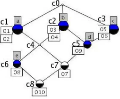
Fig. 5.Concept lattice.
to be filtered and exploration to be stopped. If function FILTER always returns (KEEP = true, CONTINUE=true), then all frequent concepts are eventually computed.
Example 5. Illustration of the computation of Exploration is as follows. The taxonomy is presented in Figure 4; Figure 5 shows the explored lattice. We assume min sup=3. The first 2 steps of computation are explained. Initially, Exploration is:
– Exploration ={(O 7→ >, ∅, ∅)}.
First step: the top of the lattice is explored, i.e. s=c0. Increments of s are computed from the taxonomy only, as there is no predecessor concept:
– incrc0 ={ {o3, o4, o7, o8, o9, o10} 7→ {b}, {o1, o2, o7, o8, o10} 7→ {a}, {o5,
o6, o7, o9, o10} 7→ {c}}
– Exploration ={({o3, o4, o7, o8, o9, o10} 7→ {b}, ∅, incrc0), ({o1, o2, o7, o8,
o10} 7→ {a}, ∅, incrc0), ({o5, o6, o7, o9, o10} 7→ {c}, ∅, incrc0)}.
Second step: an element of Exploration with the largest possible extent is explored: s = c2, p(s) = c0. In order to compute incrc2, we have to consider the
elements of incrc0 and the elements in the taxonomy.
– incrc2 ={ {o7, o8, o10} 7→ {a}, {o7, o9, o10} 7→ {c, d}, {o///////////////8, o10} 7→ {e}}
– Exploration ={( {o1, o2, o7, o8, o10} 7→ {a}, ∅, incrc0), ({o5, o6, o7, o9,
o10} 7→ {c}, ∅, incrc0), ({o7, o9, o10} 7→ {c,d}, {b}, incrc2), ({o7, o8, o10}
7→ {a}, {b}, incrc2)}.
In the second step, attributes d and e are introduced as successors of at-tributes b, and atat-tributes a and c are introduced as increments of c0, the prede-cessor of c2.
Increment{e} is eliminated because it leads to an unfrequent concept. At-tributes c and d are grouped into a single increment because they lead to the same subconcept. This ensures that computed intents are complete.
3.3 Comparison with Bordat’s algorithm
The algorithm presented in the previous section is based on Bordat’s algorithm. Like in Bordat’s version, our algorithm starts by exploring the top concept. Then for each concept s explored, the subconcepts of s are computed; this corresponds to the computation of incrs. Our algorithm uses the same data structure to rep-resent Solution, i.e. a trie. The differences between our algorithm and Bordat’s are: 1) the strategy of exploration, 2) the data structure of Exploration and 3) taking into account the taxonomy.
In our algorithm,
1. we first explore concepts in Exploration with the largest extent. Thus, it is a top-down exploration of the concept lattice, where each concept is explored only once. Contrary to Bordat, it avoids to test if a concept has already been found when it is added to Solution.
2. Whereas in Bordat’s algorithm Exploration is represented by a queue that contains subconcepts to explore, in our version the data structure of Ex-ploration elements is a triple: (exts7→ X, intp(s), incrp(s)) where incrp(s) avoids to test all attributes of the context when computing increments of s. Indeed, if an increment X is not relevant for p(s) it cannot be relevant for s, because exts⊂ extp(s) and thus (exts∩ ext(X)) ⊂ (extp(s)∩ ext(X)). Thus, the relevant increments of the predecessor of s are stored in incrp(s) and are potential increments of s. In Exploration, a concept cannot be represented several times. When a triple representing a concept c is added to Exploration, if c is already represented in Exploration, the new triple erases the previous one.
3. The attributes can be structured in a taxonomy. This taxonomy is taken into account during the computation of the increments and the intents. Us-ing∪tax instead of the plain set-theoretic union operation allows computed intents to be without redundancy. Another benefit is that it makes com-putation more efficient. For instance, when the taxonomy is deep, a lot of attributes can be pruned without testing.
4
Instantiations of the Parameterized Algorithm
In the previous section, the presented algorithm is parameterized with a filter function in order to permit the computation of concept-based rules in FCA-Tax. In this section, we show two instantiations of the filter function to learning. The first one allows sufficient conditions to be computed. Sufficient conditions are premises of rules where the conclusion (the target), W , represents the positive examples. In other words, the searched rules are of the form X → W .
The second one allows incompatible conditions to be computed. Incompatible conditions are premises of rules where the conclusion (the target), W , is the negation of the intent of positive examples. In other words, the searched rules are of the form X → ¬W .
4.1 Computing sufficient conditions
In the generation of sufficient conditions, the learning objective, W , is the tar-get of the rules to be learned. For computing sufficient conditions, one must determine what conjunctions of attributes, X, implies W , i.e. the intents X of concepts such that the rule X→ W has a support and a confidence greater than the thresholds min sup and min conf . Sufficient conditions can be computed with the algorithm described in Section 3 that filters all frequent concepts of a context, by instantiating the filter function with:
FILTERsc(exts, ext(W )) = (KEEP = sup(ints→ W ) ≥ min sup ∧ conf (ints→ W ) ≥ min conf, CONTINUE = sup(ints→ W ) ≥ min sup) It implies three possible behaviours of the algorithm.
1. The concept s is relevant, i.e. the rule ints → W has a support and a confidence greater than the thresholds. s is a solution and has to be kept, and its subconcepts are potential solutions and have to be explored. Thus FILTERsc(exts) returns (true, true).
2. The concept s has a support greater than min sup but a confidence lower than min conf . s is not a solution but the confidence is not monotonous and thus subconcepts of s can be solutions. FILTERsc(exts) returns (f alse, true). 3. The concept s has a support lower than min sup. s is not a solution. As the
support is monotonous, i.e. the support of a subconcept of s is lower than the support of s, subconcepts of s cannot be solutions. FILTERsc(exts) returns (f alse, f alse).
FILTERsc(exts, ext(W )) can be expressed in terms of extent by simply applying the definitions of support and confidence seen in Section 2. The filter function can therefore be defined by :
FILTERsc(exts, ext(W )) = (KEEP =kexts∩ ext(W )k ≥ min sup ∧ kexts∩ ext(W )k
kextsk ≥ min conf, CONTINUE =kexts∩ ext(W )k ≥ min sup) Note that it is easy to use other statistical indicators like lift or conviction, by adding conditions in the evaluation of KEEP.
4.2 Computing incompatible conditions
In the case of incompatible conditions, the learning objective, W , is the negation of the target of the rules to be learned. For computing incompatible conditions, one must determine what conjunctions of attributes, X, implie ¬W . In other words, one looks for the intents X of concepts such that the rule X → ¬W has a support and a confidence greater than the thresholds min sup and min conf .
Incompatible conditions can be computed with the algorithm described in Sec-tion 3 by instantiating the filter funcSec-tion with:
FILTERic(exts, ext(W )) = (KEEP = sup(ints→ ¬W ) ≥ min sup ∧ conf (ints→ ¬W ) ≥ min conf, CONTINUE = sup(ints→ ¬W ) ≥ min sup) As for sufficient conditions, this can be expressed in terms of extents, using the definitions of support and confidence. The filter function to compute incompat-ible conditions can thus be defined by :
FILTERic(exts, ext(W )) = (KEEP =kexts∩ (O \ ext(W ))k ≥ min sup ∧ kexts∩ (O \ ext(W ))k
kextsk ≥ min conf,
CONTINUE =kexts∩ (O \ ext(W ))k ≥ min sup)
5
Experiments
Experimental settings. The algorithm is implemented in CAML (a functional programming language of the ML family) inside the Logic File System
LISFS [PR03]. LISFS implements the notion of Logical Information Systems (LIS) as a native Linux file system. Logical Information Systems (LIS) are based on LCA. In LISFS, attributes can be ordered to create a taxonomy (logical ordering). The data structures which are used allow taxonomies to be easily manipulated. For more details see [PR03]. We ran experiments on an Intel(R) Pentium(R) M processor 2.00GHz with Fedora Core release 4, 1GB of main memory.
We tested the parameterized algorithm with two contexts: “Mushroom” and “Java”. The Mushroom benchmark3 contains 8 416 objetcs which are rooms. The mushrooms are described by properties such as whether the mush-room is edible or poisonous, the ring number, or the veil color. The context has 127 properties. The Java context4 taken from [SR06], contains 5 526 objects which are the methods of java.awt. Each method is described by its input and output types, visibility modifiers, exceptions, keywords extracted from its iden-tifiers, and keywords from its comments. The context has 1 624 properties, and yields about 135 000 concepts.
Quantitative Experiments. Many efficient algorithms computing association rules exist5. None of them allow a taxonomy to be taken into account. We do not pretend that our algorithm is faster. The objectives of this section are rather to show 1) that our algorithm is reasonably efficient, 2) that given an algorithm
3 Available at ftp://ftp.ics.uci.edu/pub/machine-learning-databases/mushroom/ 4 Available at http://lfs.irisa.fr/demo-area/awt-source/,
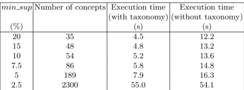
min supNumber of concepts Execution time Execution time (with taxonomy) (without taxonomy)
(%) (s) (s) 20 35 4.5 12.2 15 48 4.8 13.2 10 54 5.2 13.6 7.5 86 5.8 14.8 5 189 7.9 16.3 2.5 2300 55.0 54.1
Table 2.Number of concepts and execution times (in seconds) for different values of min sup.
which searches for association rules, the additional mechanisms described in Sections 3 and 4 do not cause any significant slowdown in the presence of a taxonomy, and 3) that they can even improve efficiency in certain cases.
We evaluate our algorithm on the mushroom benchmark, computing frequent concepts. It enables us to compare our algorithm’s performance with Pasquier et al.’s CLOSE algorithm, using the figures published in Pasquier’s PhD the-sis [Pas00]. For the same task, execution times are of the same order for both algorithms. For instance, with min sup = 5% CLOSE computation time is about 210s and our algorithm computation time is 290.8s; with min sup = 20% CLOSE computation time is about 50s and our algorithm computation time is only 26.2s. Hence, even without a taxonomy our algorithm does not introduce any slowdown. On the Java context, we measured the computation time of the frequent concepts, in order to show the impact of the taxonomy on the computation. The taxonomy is derived, for the largest part, from the class inheritance graph, and, for a smaller part, from a taxonomy of visibility modifiers that is predefined in Java. The result is given in Table 2. The third column of that table contains the execution times in seconds of algorithm when the taxonomy is taken into account. The fourth column corresponds to the execution times when the context is a priori completed with the elements of the taxonomy. When min sup = 5%, 189 frequent concepts are computed in 8s with taxonomy, whereas they are computed in 16s without taxonomy. When min sup = 2.5%, 2300 frequent concepts are computed in 55s with taxonomy, whereas they are computed in 54s without taxonomy. It is explained by the fact that the Java context has few very frequent concepts. Thus pruning using the taxonomy when min sup is greater than 5% occurs very early in the traversal of the concept lattice. For min sup = 2.5%, pruning are less impact, computation time is therefore equivalent with or without taxonomy.
Note that from a qualitative point of view, with this context, using the tax-onomy allows the number of irrelevant attributes in the intents to be reduced by 39% for min sup = 5%.
6
Conclusion
In this article we have proposed an algorithm parameterized by a filter func-tion to explore frequent concepts in a context with taxonomy in order to learn association rules. We have described how to instantiate the filter function in order to find premises of rules where the target are positive examples (sufficient conditions) and negative examples (incompatible conditions). Quantitative ex-periments have shown that, in practice, taking a taxonomy into account does not negatively impact the performance and can even make the computation more efficient.
The advantage of the presented method is to avoid the redundancies that a taxonomy may introduce in the intents of the frequent concepts.
References
[AIS93] Rakesh Agrawal, Tomasz Imielinski, and Arun Swami. Mining associations between sets of items in massive databases. In Proc. of the ACM-SIGMOD 1993 Int. Conf. on Management of Data, pages 207–216, May 1993. [AS94] Rakesh Agrawal and Ramakrishnan Srikant. Fast algorithms for mining
association rules. In Proc. 20th Int. Conf. Very Large Data Bases, VLDB, pages 487–499, 12–15 1994.
[BMUT97] Sergey Brin, Rajeev Motwani, Jeffrey D. Ullman, and Shalom Tsur. Dy-namic itemset counting and implication rules for market basket data. In Joan Peckham, editor, Proc. ACM SIGMOD Int. Conf. on Management of Data, pages 255–264. ACM Press, 05 1997.
[Bor86] J. Bordat. Calcul pratique du treillis de Galois d’une correspondance. Math´ematiques, Informatiques et Sciences Humaines, 24(94):31–47, 1986. [CFRD06] Peggy Cellier, S´ebastien Ferr´e, Olivier Ridoux, and Mireille Ducass´e. An
algorithm to find frequent concepts of a formal context with taxonomy. In Concept Lattices and Their Applications, 2006.
[FR04] S´ebastien Ferr´e and Olivier Ridoux. An introduction to logical information systems. Information Processing & Management, 40(3):383–419, 2004. [GW99] Bernhard Ganter and Rudolf Wille. Formal Concept Analysis: Mathematical
Foundations. Springer-Verlag, 1999.
[Kuz04] Sergei O. Kuznetsov. Machine learning and formal concept analysis. In International Conference Formal Concept Analysis, pages 287–312, 2004. [Mit97] Tom Mitchell. Machine Learning. McGraw-Hill, 1997.
[Pas00] Nicolas Pasquier. Data Mining : Algorithmes d’extraction et de r´eduction des r`egles d’association dans les bases de donn´ees. Computer science, Uni-versit´e Blaise Pascal - Clermont-Ferrand II, January 2000.
[PBTL99] Nicolas Pasquier, Yves Bastide, Rafik Taouil, and Lotfi Lakhal. Discovering frequent closed itemsets for association rules. In Proc. of the 7th Int. Conf. on Database Theory, pages 398–416. Springer-Verlag, 1999.
[PR03] Yoann Padioleau and Olivier Ridoux. A logic file system. In Proc. USENIX Annual Technical Conference, 2003.
[SR06] Benjamin Sigonneau and Olivier Ridoux. Indexation multiple et automa-tis´ee de composants logiciels. Technique et Science Informatiques, 2006. [Zak04] Mohammed J. Zaki. Mining non-redundant association rules. Data Mining