Adversarially-learned inference via an ensemble of discrete undirected graphical models

Adversarially-learned Inference via an Ensemble of

Discrete Undirected Graphical Models

by

Adarsh Keshav S. Jeewajee

B.S. Computer Science and Engineering

Massachusetts Institute of Technology, 2018

Submitted to the Department of Electrical Engineering and Computer

Science

in partial fulfillment of the requirements for the degree of

Master of Engineering in Electrical Engineering and Computer Science

at the

MASSACHUSETTS INSTITUTE OF TECHNOLOGY

September 2020

c

○ Massachusetts Institute of Technology 2020. All rights reserved.

Author . . . .

Department of Electrical Engineering and Computer Science

August 14, 2020

Certified by . . . .

Leslie Pack Kaelbling

Panasonic Professor of Computer Science and Engineering

Thesis Supervisor

Accepted by . . . .

Katrina LaCurts

Chair, Master of Engineering Thesis Committee

Adversarially-learned Inference via an Ensemble of Discrete

Undirected Graphical Models

by

Adarsh Keshav S. Jeewajee

Submitted to the Department of Electrical Engineering and Computer Science on August 14, 2020, in partial fulfillment of the

requirements for the degree of

Master of Engineering in Electrical Engineering and Computer Science

Abstract

Undirected graphical models are compact representations of joint probability distri-butions over random variables. To carry out an inference task of interest, graphical models of arbitrary topology can be trained using empirical risk minimization. How-ever, when faced with new tasks, these models (EGMs) often need to be re-trained. Instead, we propose an inference-agnostic adversarial training framework for producing an ensemble of graphical models (AGMs). The ensemble is optimized to generate data, and inference is learned as a by-product of this endeavor. AGMs perform comparably with EGMs on inference tasks that the latter were specifically optimized for. Most importantly, AGMs show significantly better generalization capabilities across inference tasks. AGMs are also on par with GibbsNet, a state-of-the-art deep neural architecture, which like AGMs, allows conditioning on any subset of random variables. Finally, AGMs allow fast data sampling, competitive with Gibbs sampling from EGMs.

Thesis Supervisor: Leslie Pack Kaelbling

Acknowledgments

I would like to thank Professor Leslie Kaelbling for her precious guidance during the research and writing processes that culminated into this thesis. Leslie always found time to meet and discuss research progress, listened enthusiastically to ideas I had to propose, and offered insightful feedback which shaped this work. Thanks to Leslie, research was fun, captivating and rewarding.

I am grateful to many other people who I have had a chance to work with, dur-ing the MEng program. Professor Polina Golland and Professor Gregory Wornell triggered my fascination with inference through their introduction to inference course, when I was an undergraduate. They allowed me to TA the course twice, helping me strengthen my grasp on topics such as graphical models, which led to this thesis subject. Professor Tomás Lozano-Pérez advised me at the beginning of the 2019-2020 school year, and together with Leslie, allowed me to TA their introduction to machine learning course, which motivated a big part of this work. Ferran Alet was a great mentor at the start of the MEng program, from whom I absorbed vast amounts of knowledge about the experimental aspect of research. Professor Patrick Winston patiently guided me through my first steps in research, with useful lessons that I applied during the MEng program.

I would like to thank my family, whose support has been instrumental through-out my education. I would like to thank my mother for her unwavering psychological support, warmth, encouragement, and for always believing in me. I would like to thank my sister for being my role model through her own research milestones, and her patience and consistency. I would like to thank my father for his sacrifices and guidance which have led us this far. Finally, I would like to dedicate this thesis to my late grandmother, who would have been the proudest person to see me graduate.

Contents

1 Introduction 9

2 Background 13

2.1 Probabilistic graphical models . . . 13

2.1.1 Definition and motivation . . . 13

2.1.2 Using PGMs for inference . . . 14

2.1.3 Training PGMs . . . 15

2.1.4 Sampling from PGMs . . . 18

2.2 Generative adversarial networks . . . 19

2.2.1 Idea . . . 19

2.2.2 Choice of objective . . . 20

2.3 Categorical sampling and differentiation . . . 20

3 Method 22 3.1 Preliminaries . . . 22

3.2 Adversarial training . . . 24

3.3 Inference using the ensemble of graphical models . . . 25

4 Experiments 27 4.1 Setup . . . 27

4.2 Experiment I: Benchmarking . . . 31

4.3 Experiment II: Generalization across inference tasks on images . . . . 35

5 Related Work 42

6 Conclusion 45

A Experimental Details 46

A.1 Architectures: . . . 46 A.2 Hyperparameters: . . . 48

List of Figures

3-1 Training: 𝐿𝜃 generates a vector of parameters Ψ from 𝑧 ∼ 𝒩 (0, 𝐼𝑚)

for the graphical model 𝐺 (𝑉, 𝐸). Belief propagation generates the belief vector 𝜇 from Ψ. In the WGAN-GP scheme (see section 3.2), ˜

𝑥 := 𝜇 is taken to be the fake data from generator 𝐺𝜃, and is fed to

discriminator 𝐷𝑤 (not pictured). . . 24

3-2 Testing/Inference: Given a query (Xℰ = 𝑥ℰ, X𝒬, Xℋ), an ensemble

of 𝑀 graphical models parametrized by Ψ𝑧1, . . . , Ψ𝑧𝑀 is produced by

𝐿𝜃 from 𝑧1, . . . , 𝑧𝑀 ∼ 𝑁 (0, 𝐼𝑚). Belief propagation on each model given

the same observations 𝑥ℰ (red nodes) produces 𝑀 conditional beliefs. 26

4-1 In columns 1 to 4, query-creation schemes are: fractional(0.85), corrupt(0.2), window(10) and quadrant(1), respectively (see section 4.1). Original data points on row 1 are converted to queries (Xℰ =

𝑥ℰ, X𝒬, Xℋ) on row 2 (non-red pixels are observations 𝑥ℰ, red pixels

are variables X𝒬 to be guessed). Row 3 shows marginals guessed by

an AGM by plotting 𝑃 (pixel = 1). Note that one AGM was able to answer all of those queries. . . 28 4-2 The Caltech-101 Silhouettes dataset (CALTECH) has images of the

silhou-ettes of objects from the Caltech-101 dataset, which span 101 categories. Pixels have value 0 or 1, indicating occlusion or not. . . 30

4-3 One data point as an example, from the daily precipitation data of the Pacific Northwest from 1949 to 1994 from Widmann and Bretherton [2000]. Each grid cell is a weather station, which adds one random variable to every data point. The fact that the random variables are regularly organized in euclidean space allows us to experiment with both random and grid graphs in experiment 4.2, for this data set. . . 30 4-4 Inference accuracies (vertical axes) obtained across datasets, using the

AGM model (experiment I), where the variable being varied in every plot is the ensemble size 𝑀 (horizontal axes) used during inference. Values used for 𝑀 were 10, 100, 1000, 10000, indicated in logarithm base 10. . . 34 4-5 Images (column 1) generated from the AGM by providing different

random latent vectors 𝑧 to models trained on MNIST (rows 1-2) and Caltech-101 (rows 3-4). Horizontally across every row, the random vectors are gradually changed to a target latent vector. Images are crisp and transition smoothly from source to target. . . 38 4-6 Images sampled from an EGM trained on the fractional(0.5) task

through Gibbs sampling involving 10 burn in cycles. . . 38 4-7 Schema illustrating the pipeline used in experiment III, with original

data from some data set D used to train AGM A and EGM B. Data is separately sampled from both. Each synthetic data set trains a separate EGM (𝐸1 and 𝐸2) from scratch. These are separately tested on the

same test data pertaining to data set D. The key box at the bottom explains the meaning of the different types of arrows used in the schema. 40

List of Tables

4.1 Characteristics of the data sets used in our experiments: Name, number of variables, size of discrete support and sizes of the [train, validation, test] splits. . . 29 4.2 Performances from experiment I on the fractional(0.7) inference task,

across candidate models. Each printed value is an average over 3 trials. 32 4.3 Cross-task accuracies (averaged over 3 trials) for EGMs, AGM, MIX

and MIX-1. Tasks trained on (where applicable), are in the first column, and test tasks for all models are on the second row. Means of the rows indicate relative generalization abilities. . . 37 4.4 Inference performances from experiment III, obtained by the EGM

evaluators, trained on data sampled from an AGM sampler, a Gibbs sampler with no burn-in and a Gibbs sampler with burn-in of 10 iterations. 39

Chapter 1

Introduction

In this work, at the highest level of abstraction, we are searching for a probability distribution ˜_{P which best describes available data. The data was sampled from the true} probability distribution P which we do not have direct access to. The data consists of several joint instantiations of random variables X1, . . . , X𝑁, with each random variable

X𝑖 taking on a value 𝑥𝑖 from a discrete set 𝒳 . ˜P should essentially be a function which

maps a specific instantiation 𝑥1, . . . , 𝑥𝑁 to a value in the range [0, 1], and the sum

across all configurations of the random variables, ∑︀

𝑥1,...,𝑥𝑁

˜

P(X1 = 𝑥1, . . . , X𝑁 = 𝑥𝑁),

should yield 1.

The reason why we would like a distribution ˜_{P is to be able to answer queries of} the form

arg max

𝑥∈𝒳 P(X

𝑖 = 𝑥|Xℰ = 𝑥ℰ), ∀𝑖 ∈ 𝒬 (1.1)

expressed in compact notation (Xℰ = 𝑥ℰ, X𝒬, Xℋ), where from a data point (𝑥1, . . . , 𝑥𝑁)

sampled from the true data distribution P, we observe the values of a subset ℰ of the indices, and have to predict the values at indices in 𝒬 from discrete set 𝒳 , with the possibility of some hidden variable indices ℋ which have to be marginalized over. A distribution over queries of this form will be referred to as an inference task.

In this work, we will constrain ˜_{P to come from the family of probabilistic graphical} models [Koller and Friedman, 2009, Murphy, 2012]. These are compact representations of joint probability distributions (section 2.1). We focus on discrete pairwise undirected

graphical models, which represent the independence structure between pairs of random variables. Algorithms such as belief propagation (section 2.1.2) allow for inference on these graphical models, with arbitrary choices of observed and hidden variables. When the graph topology is loopy, or when the structure is mis-specified, inference through belief propagation is approximate [Murphy et al., 2013].

A purely generative way to train such a model is to maximize the likelihood of training data (ML) (section 2.1.3), under the probability distribution induced by the model. However, evaluating the gradient of this objective involves computing marginal probability distributions over the random variables. As these marginals are approxi-mate in loopy graphs, the applicability of likelihood-trained models to discriminative tasks, such as answering queries as expressed in equation 1.1 is diminished [Kulesza and Pereira, 2008].

If the distribution over queries that the model will be called upon to answer is known, then the model’s performance can be improved by shaping the query distribution used at parameter estimation time, accordingly. In degenerate tasks, ℰ , 𝒬 and ℋ are fixed across queries. When this is the case and ℋ is empty, we could use a Bayesian feed-forward neural network [Husmeier and Taylor, 1999] to model the distribution in (1.1) and train it by backpropagation. The empirical risk minimization of graphical models (EGM) framework of Stoyanov et al. [2011] and Domke [2013] generalizes this gradient-based parameter estimation idea to graphical models. Their framework allows retaining any given graphical model structure, and back-propagating through a differentiable inference procedure to obtain model parameters that facilitate the query-evaluation problem (section 2.1.3). EGM allows solving the most general form of problems expressed as (1.1), where ℰ , 𝒬 and ℋ are allowed to vary. Information about this query distribution is used at training time to sample choices of evidence and query variable indices (ℰ , 𝒬), as well the observed values 𝑥ℰ across data points.

They then train the whole imperfect system end-to-end through gradient propagation [Domke, 2010]. This approach improves the inference accuracy on this specific query distribution, by orders of magnitude compared to the ML approach. One significant drawback of the EGM approach is that the training procedure is tailored to one

specific inference task. To solve a different inference task, the model often has to be completely re-trained (section 4).

Instead, we would like to learn discrete undirected graphical models which generalize over different or multi-modal inference tasks. Our adversarially trained graphical model (AGM) strategy is built on the GAN framework [Goodfellow et al., 2014]. It allows us to formulate a learning objective for our graphical models, aimed purely at optimizing the generation of samples from the model. No information about inference tasks is baked into this learning approach. Our only assumption during training is that the training and testing data points come from the same underlying distribution. Although our undirected graphical models need to be paired to a neural learner for the adversarial training, they are eventually detached from the learner, with an ensemble of parameterizations. When using one of the parameterizations, our graphical model is indistinguishable from one that was trained using alternative methods. We propose a mechanism for performing inference with the whole ensemble, which provides the desired generalization properties across inference tasks, improving over EGM performance. Our learning approach is essentially generative, but the ensemble of models increases the expressive power of the final model, making up for approximations in inference and model mis-specification which affected the ML approach discussed above.

In the next sections, we summarize background concepts which our work builds up on (2), and introduce our adversarial training framework (3) for undirected graphical models. Our first experiment (4.2), shows that although undirected graphical models with empirical risk minimization (EGMs) are trained specifically for certain inference tasks, our adversarially-trained graphical models (AGMs) can perform comparatively, despite having never seen those tasks prior to training. We also show that the AGM’s inference performance is on par with GibbsNet’s [Lamb et al., 2017], a state-of-the-art deep adversarially-trained neural inference network. The second experiment (4.3) showcases the generalization capabilities of AGMs across unseen inference tasks on images. In the last experiment (4.4), we show that the combination of AGMs and their neural learner provide a viable alternative for sampling from joint probability

distributions in one shot, compared to Gibbs samplers defined on EGMs. We finally discuss work related to ours (5) and possible directions in which our work can be extended (6).

Chapter 2

Background

This section briefly discusses concepts that are used or extended in our work. For a deeper discussion about these background concepts, relevant papers are cited.

2.1

Probabilistic graphical models

2.1.1

Definition and motivation

As motivated in section 1, in this work, we would like to find a probability distribution ˜

P which best describes available data which is sampled from some true probability distribution P. A probabilistic graphical model essentially gives us one candidate formulation for the function ˜_P:

˜ P(X1 = 𝑥1, . . . , X𝑁 = 𝑥𝑁) = 1 𝒵 ∏︁ (𝑖,𝑗)∈𝐸 𝜓𝑖,𝑗(𝑥𝑖, 𝑥𝑗), (2.1)

(which is re-expressed in 3.1 to adhere to the notation of that section).

It is useful to think of the random variables X1, . . . , X𝑁 as forming a graph 𝒢(𝑉, 𝐸)

with node set 𝑉 consisting of one node for every random variable, and edge set 𝐸 consisting of pairs of random variables which are connected on the graph by an edge. Every pair of random variables which share an edge (X𝑖, X𝑗) are assigned a

assignment X𝑖 = 𝑥𝑖, X𝑗 = 𝑥𝑗. We note that expression 2.1 yields probabilities up to a normalization constant 𝒵 = ∑︁ 𝑥1,...,𝑥𝑁 ∏︁ (𝑖,𝑗)∈𝐸 𝜓𝑖,𝑗(𝑥𝑖, 𝑥𝑗). (2.2)

Computing 𝒵 requires summing over |𝒳 |𝑁 _{terms. This sum can be simplified}

signif-icantly for tree graphs by taking advantage of the specific factorization that arises in equation 2.1. However, as we are interested in graphs of arbitrary topology, we cannot assume such simplifications, and therefore it will be intractable to compute 𝒵. Similarly, from the joint probabilities ˜_P(X1 = 𝑥1, . . . , X𝑁 = 𝑥𝑁) which are known up

to the normalization constant 𝒵, computing marginal probabilities over single random variables, will require suming over |𝒳 |𝑁 −1_{terms and exact marginalization is therefore}

also intractable.

2.1.2

Using PGMs for inference

However, as was motivated in section 1, we will need marginal probability distributions 𝑝𝑋𝑖(𝑥𝑖) to answer queries of the form shown in equation 1.1. We will have to resort to

approximations of these marginals, obtained by carrying out the belief propagation algorithm. It is a message-passing algorithm with the ultimate goal of approximating the marginals for every random variable. Messages are sent back and forth across every edge, iteratively. A messages, from node 𝑖 to node 𝑗, can be thought of as a ‘partial marginalization computation’ done locally at node 𝑖, combining information from its neighborhood 𝑁 (𝑖) and passed on to node 𝑗 as a function defined over the support of node 𝑗, as:

𝑚(𝑡+1)_𝑖→𝑗 (𝑥𝑗) = ∑︁ 𝑥𝑖 𝜓𝑖,𝑗(𝑥𝑖, 𝑥𝑗) ∏︁ 𝑘∈𝑁 (𝑖):𝑘̸=𝑗 𝑚(𝑡)_𝑘→𝑖(𝑥𝑖). (2.3)

While these messages will eventually converge on tree graphs, no convergence guarantee exists for graphs of arbitrary topology which we are interested in [Murphy et al., 2013], hence in our work we carry out the message passing as shown in 2.3 for a fixed number

of iterations 𝑇 (section 3.1), after which we compute approximate marginal probability distributions at every node as:

ˆ

𝑝X𝑖(𝑥𝑖) =

∏︁

𝑗∈𝑁 (𝑖)

𝑚(𝑇 )_𝑗→𝑖(𝑥𝑖). (2.4)

We note that one can also perform inference in scenarios where a fraction of the variables being modelled is already observed. In this case, the value of any observed random variable X𝑖 will be frozen to its observed value 𝑥′𝑖 in every edge potential

involving that variable.

2.1.3

Training PGMs

To motivate to our novel method for training PGMs, it is worth taking a look at existing learning methods and their limitations.

As generative models

First, it is natural when given any probabilistic model, to tune its parameters in a purely generative way, for example by maximizing the (log) likelihood of training data, under the probability distribution induced by the model. Assuming 𝑀 data points 𝒟 = {(𝑥(1)₁ , . . . , 𝑥(1)_𝑁 ), . . . , (𝑥(𝑀 )₁ , . . . , 𝑥(𝑀 )_𝑁 )}, the (log) likelihood of data 𝒟 under the model parameterized by edge potentials summarized by Ψ is given by:

log ℒ(𝒟; Ψ) = log 𝑀 ∏︁ 𝑘=1 ˜ P(X1 = 𝑥 (𝑘) 1 , . . . , X𝑁 = 𝑥 (𝑘) 𝑁 ) = log 𝑀 ∏︁ 𝑘=1 1 𝒵 ∏︁ (𝑖,𝑗)∈𝐸 𝜓𝑖,𝑗(𝑥 (𝑘) 𝑖 , 𝑥 (𝑘) 𝑗 ) = 𝑀 ∑︁ 𝑘=1 ∑︁ (𝑖,𝑗)∈𝐸 log 𝜓𝑖,𝑗(𝑥 (𝑘) 𝑖 , 𝑥 (𝑘) 𝑗 ) − 𝑀 log 𝒵

(𝑋𝑖, 𝑋𝑗) takes on the configuration (𝑥𝑖, 𝑥𝑗) ∈ (𝒳 × 𝒳 ) in our data set, we can simplify

the expression into a form which is more convenient differentiation:

log ℒ(𝒟; Ψ) = ∑︁

(𝑖,𝑗)∈𝐸

∑︁

(𝑥𝑖,𝑥𝑗)∈(𝒳 ×𝒳 )

𝑐(𝑥𝑖, 𝑥𝑗) log 𝜓𝑖,𝑗(𝑥𝑖, 𝑥𝑗) − 𝑀 log 𝒵

One observation is that the intractable normalization constant 𝒵 is present in this likelihood. To maximize the likelihood with respect to the model parameters, we need the gradient _𝜕𝜓 𝜕ℒ

𝑎,𝑏(𝑥𝑎,𝑥𝑏) for all (𝑎, 𝑏) ∈ 𝐸 and all assignments (𝑥𝑎, 𝑥𝑏) ∈ (𝒳 × 𝒳 ), to

perform gradient ascent. First, 𝜕 𝜕𝜓𝑎,𝑏(𝑥𝑎, 𝑥𝑏) ∑︁ (𝑖,𝑗)∈𝐸 ∑︁ (𝑥𝑖,𝑥𝑗)∈(𝒳 ×𝒳 ) 𝑐(𝑥𝑖, 𝑥𝑗) log 𝜓𝑖,𝑗(𝑥𝑖, 𝑥𝑗) = 𝑐(𝑥𝑎, 𝑥𝑏) 𝜓(𝑥𝑎, 𝑥𝑏) , and second, 𝜕 𝜕𝜓𝑎,𝑏(𝑥𝑎, 𝑥𝑏) 𝑀 log 𝒵 = 𝑀 𝒵 𝜕 𝜕𝜓𝑎,𝑏(𝑥𝑎, 𝑥𝑏) 𝒵 = 𝑀 𝒵 𝜕 𝜕𝜓𝑎,𝑏(𝑥𝑎, 𝑥𝑏) ∑︁ 𝑥′₁,...,𝑥′_𝑁 ∏︁ (𝑖,𝑗)∈𝐸 𝜓𝑖,𝑗(𝑥𝑖, 𝑥𝑗) = 𝑀 𝒵 ∑︁ 𝑥′ 1,...,𝑥′𝑁:𝑥′𝑎=𝑥𝑎,𝑥′_𝑏=𝑥𝑏 𝜕 𝜕𝜓𝑎,𝑏(𝑥𝑎, 𝑥𝑏) ∏︁ (𝑖,𝑗)∈𝐸 𝜓𝑖,𝑗(𝑥𝑖, 𝑥𝑗) = 𝑀 𝒵 ∑︁ 𝑥′₁,...,𝑥′_𝑁:𝑥′ 𝑎=𝑥𝑎,𝑥′_𝑏=𝑥𝑏 ∏︁ (𝑖,𝑗)∈𝐸∖(𝑎,𝑏) 𝜓𝑖,𝑗(𝑥𝑖, 𝑥𝑗) = 𝑀 𝒵 𝜓𝑎,𝑏(𝑥𝑎, 𝑥𝑏) 𝜓𝑎,𝑏(𝑥𝑎, 𝑥𝑏) ∑︁ 𝑥′ 1,...,𝑥′𝑁:𝑥 ′ 𝑎=𝑥𝑎,𝑥′_𝑏=𝑥𝑏 ∏︁ (𝑖,𝑗)∈𝐸∖(𝑎,𝑏) 𝜓𝑖,𝑗(𝑥𝑖, 𝑥𝑗) = 𝑀 1 𝜓𝑎,𝑏(𝑥𝑎, 𝑥𝑏) ∑︁ 𝑥′₁,...,𝑥′_𝑁:𝑥′ 𝑎=𝑥𝑎,𝑥′𝑏=𝑥𝑏 1 𝒵 ∏︁ (𝑖,𝑗)∈𝐸 𝜓𝑖,𝑗(𝑥𝑖, 𝑥𝑗) = 𝑀𝑝X𝑎,X𝑏(𝑥𝑎, 𝑥𝑏) 𝜓𝑎,𝑏(𝑥𝑎, 𝑥𝑏)

The problem of the intractable 𝒵 appearing in the likelihood, intuitively, should not magically disappear as we differentiate the likelihood. Indeed, the marginal

probability 𝑝X𝑎,X𝑏(𝑥𝑎, 𝑥𝑏) arises in the expression for the gradient of the likelihood

with respect to the parameters 𝜓(𝑥𝑎, 𝑥𝑏). (We note that extending this method to

the case where there are hidden variables (variables that are not observed in the data points) requires replacing those variables with their expectations, which leads to the expectation maximization method which will also suffer from the need for marginals.) We concluded that this marginal is intractable to compute in section 2.1.1, hence we have to rely on its approximation to obtain gradients, but these approximations, together with the fact that the graph structure itself is often an approximation in applications, causes the parameters obtained by gradient ascent to not necessarily be the best, as initially argued by Kulesza and Pereira [2008] and empirically verified by Domke [2013].

Empirical risk minimization

The method more commonly used to train PGMs which are eventually used dis-criminatively, is empirical risk minimization, which is an ‘inference-aware’ method. Our work treats this method as a baseline. Stoyanov et al. [2011] and Domke [2013] proposed this method, which treats PGMs, and the larger inference pipeline which they are a part of, as one black box, whose parameters have to be optimized, such that its outputs minimize some empirical risk of interest. This method is applicable when the computational process from the inputs to the outputs of this black box is fully differentiable, and these papers focus specifically on cases where the inference procedure being used on the PGM is belief propagation (section 2.1.2).

Concretely, say a PGM needs to be trained so that it can answer queries of the form shown in equation 1.1, where given some data point (𝑥(𝑘)₁ , . . . , 𝑥(𝑘)_𝑁 ), a fraction 𝒬(𝑘) _{of the random variables X}

1, . . . , X𝑁 is to be inferred given the rest (𝑉 ∖ 𝒬(𝑘))

by belief propagation carried out for 𝑇 iterations, and the accuracy of this inference task is to be quantified by some loss function ℒ taking in the approximate marginals ˆ

𝑝(𝑘)_𝑖 (𝑥𝑖) produced by belief propagation at the random variables 𝑖 ∈ 𝒬(𝑘), with the

true values 𝑥(𝑘)_𝑖 of these variables given by the data point. The belief propagation process (and hence its produced marginals) is differentiable with respect to PGM

parameters. As long as the loss function ℒ is differentiable with respect to its inputs, then under the empirical risk minimization method, one would perform the following optimization (assuming a training data set of interest is used to formulate 𝐾 queries in all) to train the PGM parameters Ψ:

Ψ* = arg min Ψ 1 𝐾 𝐾 ∑︁ 𝑘=1 ∑︁ 𝑖∈𝒬(𝑘) ℒ(ˆ𝑝(𝑘)_𝑖 (𝑥𝑖), 𝑥 (𝑘) 𝑖 ). (2.5)

The differentiability with respect to the model parameters ensures that one can use backpropagation, obtained out of the box using automatic differentiation learning packages like Paszke et al. [2019] to train these models end to end. This approach improves performances on the type of queries seen during training, by orders of magni-tude compared to the maximum likelihood and expectation maximization approaches. One significant drawback of this learning approach, however, is that it is tailored to a specific distribution over queries, i.e. the specific method that was used to generate the sets of query indices 𝒬(𝑘) in equation 2.5 (section 1 defines query distributions). To perform inference over drastically different querie distributions, the model often has to be completely re-trained (section 4).

2.1.4

Sampling from PGMs

Given a fully trained PGM, one essentially has a compact representation of a probability distribution ˜_{P over random variables. Data (concrete instantiations of these random} variables) can be sampled from the model by the process of Gibbs Sampling which is relevant in section 4.4.

The goal in Gibbs sampling is for the obtained samples to be obtained i.i.d. from ˜_P. The sampling process is iterative. Each iteration consists of sampling the value of one random variable X𝑖 given concrete assignments to all the other variables X𝑉 ∖{𝑖}. With

the values of the other variables known, the joint distribution function (2.1) simplifies to a function over the discrete support of variable X𝑖 only and the normalization

cycle is completed when all the variables have been iterated over, producing a data sample. The cycle then repeats, with this new data sample as the starting point, generating the next sample. The very first starting point is picked randomly.

The first few samples are thrown away for a fixed number of iterations 𝑏 which we call the burnin period, and from then on, every 𝑘𝑡ℎ sample is kept. Both 𝑏 and 𝑘 are chosen empirically, and 𝑏 is used to allow the sampling process to move away from the randomly picked starting point and start producing samples from the actual joint ˜_P, while 𝑘 is used to allow the samples to actually be i.i.d. despite the fact that samples form a chain.

2.2

Generative adversarial networks

2.2.1

Idea

The Generative Adversarial Networks (GANs) framework as originally introduced in [Goodfellow et al., 2014] facilitates the learning of generative models mapping typically-lower-dimensional latent vectors 𝑧 ∈ R𝑚 _{to high-dimensional data 𝑥 ∈ R}𝑛

through a generator 𝐺. Formally, 𝐺 is trained by maximizing a real-valued objective 𝑉 which involves the outputs of a discriminator function 𝐷 on data from a target data distribution P, and generated samples 𝐺(𝑧) (from the distribution Q induced by the 𝐺). 𝐷 is a function mapping data points 𝑥 ∈ R𝑛 _{to the space of real numbers.}

The objective 𝑉 is designed so that it reduces to a probabilistic distance metric of choice between P and Q, under certain conditions. By driving this objective down, the generator will get Q as close as possible to P. Commonly, one of the conditions for the objective 𝑉 to reduce to probabilistic distances of interest is that the discriminator has to be optimal. In most learning problems however, the practitioner does not possess such a discriminator and will learn both the generator and the discriminator at the same time. 𝐷 will be trained to maximize the objective 𝑉 and keep the distinction between P and Q. Hence, the overall problem reduces to a min-max optimization of 𝑉 by 𝐺 and 𝐷 respectively.

2.2.2

Choice of objective

[Nowozin et al., 2016] showed that an objective 𝑉 can be designed such that it reduces to any f-divergence metric of choice at the limit of an optimal discriminator, among other conditions. The 𝑉 (𝐷, 𝐺) objective typically used was introduced in Goodfellow et al. [2014] and is shown to be equal to reduce to a scaled and shifted version of the Jensen-Shannon divergence, in the limit of an optimal discriminator which outputs values in the range [0, 1]:

𝑉 (𝐷, 𝐺) = E𝑥∼P[log 𝐷(𝑥)] + E𝑥∼Q[log(1 − 𝐷(𝑥))].

In our work, we will use the objective from the Gulrajani et al. [2017] paper:

𝑉 (𝐷, 𝐺) = E ˜ 𝑥∼Q [𝐷𝑤(˜𝑥)] − E𝑥∼P [𝐷𝑤(𝑥)] + 𝜆 E𝑥′_∼P′ [︁ (∇𝑥′‖𝐷_𝑤(𝑥′)‖ 2 − 1) 2]︁ .

This objective is equivalent to the Wasserstein-1 (earth-mover) distance between P and Q as long as we have an optimal discriminator mapping to the whole set of real numbers and the discriminator is from the set of 1-Lipschitz functions. A differentiable function is 1-Lipschitz if and only if it has gradients with norm at most 1 everywhere. As it is intractable to mathematically compute the gradient norm of the discriminator outputs at every point, the Lipschitz constraint is enforced, by penalizing the gradient norm at random points interpolated between real and generated points.

2.3

Categorical sampling and differentiation

In our work we calibrate the parameters of a discrete probability distribution over data. We will sample from this distribution, and we would like the samples (and functions of those samples) to be differentiable with respect to the parameters of the distribution. For continuous probability distributions, like in the Gaussian case, this can be done through the Gaussian reparametrization trick [Kingma, 2013]. In our case, we are interested in categorical sampling from a discrete probability distribution. One

option is to reparametrize using the gumbel-softmax method [Jang et al., 2017], which we found to be rather unstable. We tried two other methods specific to distributions trained adversarially. First, the [Hjelm et al., 2017] formulation (reminescent of REINFORCE [Sutton et al., 1999] and importance sampling [Tokdar and Kass, 2010]) allows the practitioner to sample non-differentiably, but an array of samples has to be collected to approximate the gradient of the mean with respect to the model parameters. (We note that similar ideas were explored in [Che et al., 2017], [Li et al., 2017] and [Bornschein and Bengio, 2014]). The second method, which gave the most stable and best performance was the one we ended up keeping. In this method from Gulrajani et al. [2017], the idea is to treat a probability distribution as a ‘soft’ sample. Concretely, if one has a probability distribution over 𝑁 variables of discrete support of size |𝒳 |, the distribution is a vector in R𝑁 |𝒳 | _{and instead of sampling categorically}

from it, this vector itself is considered the sample, and is used downstream in our pipeline. This means that actual ‘hard’ data samples in R𝑁 _{have to be modified.}

Every one of their entries has to be one-hot encoded, to eventually satisfy the R𝑁 |𝒳 | format. This idea is important in section 3.2.

Chapter 3

Method

3.1

Preliminaries

We aim to learn the parameters for pairwise discrete undirected graphical models, adversarially. These models are structured as graphs 𝐺(𝑉, 𝐸), with each node in their node set 𝑉 representing one variable in the joint probability distribution being modeled (section 2.1.1). The distribution is over variables X𝑁₁ := (X1, . . . , X𝑁). For

simplicity, we assume that all random variables can take on values from the same discrete set 𝒳 .

A graphical model carries a parameter vector Ψ. On each edge (𝑖, 𝑗) ∈ 𝐸, there is one scalar 𝜓𝑖,𝑗 for every pair of values (𝑥𝑖, 𝑥𝑗) that the pair of connected random

variables can admit. Therefore every edge carries |𝒳 |2 _{parameters, and in all, the}

graphical model 𝐺 (𝑉, 𝐸) carries 𝑘 = |𝐸||𝒳 |2 total parameters, all contained in the vector Ψ ∈ R𝑘_.

Through its parameter set Ψ, the model summarizes the joint probability distri-bution over the random variables up to a normalization constant 𝒵 as follows (see section 2.1 for more information):

𝑞_X𝑁 1 (︀𝑥 𝑁 1 ; Ψ)︀ = 1 𝒵 ∏︁ (𝑖,𝑗)∈𝐸 𝜓𝑖,𝑗(𝑥𝑖, 𝑥𝑗) . (3.1)

model 𝐺 (𝑉, 𝐸), our method trains an uncountably infinite ensemble of graphical model parameters, adversarially. In our framework, our model admits a random vector 𝑧 ∈ R𝑚 sampled from a standard multivariate Gaussian distribution as well as a deterministic transformation 𝐿𝜃, from 𝑧 to a graphical model parameter vector

Ψ𝑧 = 𝐿𝜃(𝑧) ∈ 𝑅𝑘, and where 𝜃 it to be trained. Under our framework, the overall

effective joint distribution over random variables X𝑁

1 can be summarized as 𝑝_X𝑁 1 (︀𝑥 𝑁 1 )︀ = ∫︁ 𝑧∈R𝑚 𝑝Z(𝑧) 𝑝X𝑁 1 |Z(︀𝑥 𝑁 1 |𝑧)︀ 𝑑𝑧 (3.2) = ∫︁ 𝑧∈R𝑚 𝑝Z(𝑧) 𝑞X𝑁 1 (︀𝑥 𝑁 1 ; 𝐿𝜃(𝑧))︀ 𝑑𝑧 (3.3)

Through adversarial training, we will learn to map random vectors 𝑧 ∈ R𝑚 _to

data samples. The only learnable component of this mapping is the transformation of 𝑧 ∈ R𝑚 _{to Ψ}

𝑧 ∈ 𝑅𝑘through 𝐿𝜃. Given Ψ𝑧, the joint distribution 𝑞X𝑁 1 (︀𝑥

𝑁

1 ; Ψ𝑧)︀ is given

in (3.1) and since the goal of adversarial training is to produce high-quality samples which are indistinguishable from real data through the lens of some discriminator, the training process is essentially priming each Ψ𝑧 = 𝐿𝜃(𝑧) to specialize on a niche

region of the domain of the true data distribution. From the point of view of Jacobs et al. [1991], we will have learnt ‘local experts’ Ψ𝑧, each specializing to a subset of the

training distribution. The entire co-domain of 𝐿𝜃 is our ensemble of graphical models.

Finally, we will use an inference procedure throughout our exposition. Com-puting exact marginal probabilities using (3.1) is intractable (section 2.1.1). Hence, whenever we are given a graphical model structure, one parameter vector Ψ and some observations 𝑥ℰ, we carry out a fixed number 𝑡 of belief propagation iterations through

the inference(𝑥ℰ, Ψ, 𝑡) procedure, to obtain one approximate marginal probability

distribution 𝜇𝑖, conditioned on 𝑥ℰ, for every 𝑖 ∈ 𝑉 . Note that the distributions 𝜇𝑖 for

𝑖 ∈ ℰ are degenerate distributions with all probability mass on the observed value of random variable X𝑖. In our work, we will use this inference procedure with ℰ = ∅

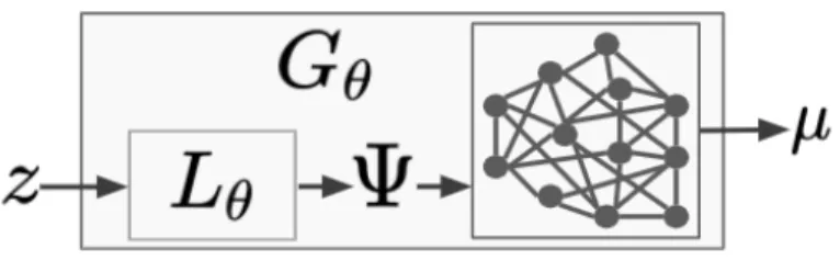
Figure 3-1: Training: 𝐿𝜃 generates a vector of parameters Ψ from 𝑧 ∼ 𝒩 (0, 𝐼𝑚) for

the graphical model 𝐺 (𝑉, 𝐸). Belief propagation generates the belief vector 𝜇 from Ψ. In the WGAN-GP scheme (see section 3.2), ˜𝑥 := 𝜇 is taken to be the fake data from generator 𝐺𝜃, and is fed to discriminator 𝐷𝑤 (not pictured).

3.2

Adversarial training

Our adversarial training framework follows Goodfellow et al. [2014] (see section 2.2.1 for more details). The discriminator 𝐷𝑤 is tasked with distinguishing between real

and fake samples in data space. Our (𝐿𝜃, 𝐺 (𝑉, 𝐸)) pair constitutes our generator

𝐺𝜃 as seen in figure 3-1. Fake samples are produced by our generator 𝐺𝜃, which as

is standard, maps a given vector 𝑧 sampled from a standard multivariate Gaussian distribution, to samples ˜𝑥.

One layer of abstraction deeper, the generative process 𝐺𝜃 is composed of 𝐿𝜃 taking

in random vector 𝑧 ∈ R𝑚 _{as input, and outputting a vector 𝑣 ∈ 𝑅}𝑘_{. The graphical}

model receives 𝑣, runs inference(𝑥ℰ = ∅, Ψ = 𝑣, 𝑡 = 𝑡′), for a pre-determined 𝑡′, and

outputs a set of marginal probability distributions 𝜇𝑖 for 𝑖 ∈ 𝑉 . Note that the set ℰ

of observed variables is empty, since our training procedure is inference-agnostic. In summary, the graphical model extends the computational process which gener-ated 𝑣 from 𝑧, with the deterministic recurrent process of belief propagation on its structure 𝐸. Note that a one-to-one correspondence from entries of 𝑣 to graphical model parameters 𝜓𝑖,𝑗(𝑥𝑖, 𝑥𝑗) has to be pre-determined for 𝐿𝜃 and 𝐺 (𝑉, 𝐸) to interface

with one another.

Instead of categorical sampling from the beliefs 𝜇𝑖 to get a generated sample for

the GAN training [Hjelm et al., 2017, Jang et al., 2017], we follow the WGAN-GP method [Gulrajani et al., 2017] for training our discrete GAN (section 2.2.2). In their formulation, the fake data point ˜𝑥 is a concatenation of all the marginal probability distributions 𝜇𝑖, in some specific order. This means that true samples from the train

data set also have to be processed into a concatenation of the 𝒳 -dimensional one-hot encodings of the values they propose for every node, to meet the input specifications of the discriminator.

We optimize the WGAN-GP objective (3.4) with the gradient ∇𝑥′‖𝐷_𝑤(𝑥′)‖

2

penalized at points 𝑥′ = 𝜖𝑥 + (1 − 𝜖)˜𝑥 which lie on the line between real samples 𝑥 and fake samples ˜𝑥. This regularizer is a tractable 1-Lipschitz enforcer on the discriminator function, which stabilizes the WGAN-GP training procedure (section 2.2.2):

min 𝑤 max𝜃 ˜𝑥∼QE [𝐷𝑤(˜𝑥)] − E𝑥∼P [𝐷𝑤(𝑥)] + 𝜆 E𝑥′_∼P′ [︁ (∇𝑥′‖𝐷_𝑤(𝑥′)‖ 2− 1) 2]︁ . (3.4)

3.3

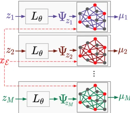
Inference using the ensemble of graphical models

Out of the various ways to coordinate responses from our ensemble of graphical model parameters (section 5), we choose the log-linear pooling method of [Antonucci et al., 2013], for its simplicity. Given a query of the form (Xℰ = 𝑥ℰ, X𝒬, Xℋ) as

seen in (1.1), we call upon a finite subset of our infinite ensemble of graphical models. We randomly sample 𝑀 random vectors 𝑧1, . . . , 𝑧𝑀 from the standard

multi-variate Gaussian distribution and map them to a collection of 𝑀 parameter vectors (Ψ1 = 𝐿𝜃(𝑧1), . . . , Ψ𝑀 = 𝐿𝜃(𝑧𝑀)). 𝑀 sets of beliefs, for every node, are fetched through

𝑀 parallel calls to the inference procedure: inference (𝑥ℰ, Ψ = 𝐿Θ(𝑧𝑗), 𝑡 = 𝑡′) for

𝑗 = 1, . . . , 𝑀 . The idea behind log-linear pooling is to aggregate the opinion of every model in our finite ensemble. Concretely, for every random variable X𝑖, its 𝑀 obtained

marginal distributions 𝜇𝑖(·|𝑥ℰ; Ψ𝑗) for 𝑗 = 1, . . . 𝑀 are aggregated as we show in (3.6):

ˆ 𝑥𝑖 = arg max 𝑥∈𝒳 𝑀 ∏︁ 𝑗=1 𝜇𝑖(𝑥|𝑥ℰ; Ψ𝑗) 1 𝑀 (3.5) = arg max 𝑥∈𝒳 1 𝑀 𝑀 ∑︁ 𝑗=1 log 𝜇𝑖(𝑥|𝑥ℰ; Ψ𝑗) . (3.6)

Figure 3-2: Testing/Inference: Given a query (Xℰ = 𝑥ℰ, X𝒬, Xℋ), an ensemble of 𝑀

graphical models parametrized by Ψ𝑧1, . . . , Ψ𝑧𝑀 is produced by 𝐿𝜃 from 𝑧1, . . . , 𝑧𝑀 ∼

𝑁 (0, 𝐼𝑚). Belief propagation on each model given the same observations 𝑥ℰ (red

Chapter 4

Experiments

4.1

Setup

For inference tasks of the type formulated in (1.1), we need strategies to create distributions over queries of the form: (Xℰ = 𝑥ℰ, X𝒬, Xℋ). We note that queries need

to be grounded in some data set of interest. In any query, observations 𝑥ℰ must come

from a real data point from a data set of choice, and the original values of query variables are kept as targets.

The query creation schemes used in our work are as follows, and we do not use hidden variables Xℋ:

(i) fractional(𝑓 ): A fraction 𝑓 of all variables are made into query variables, and the rest are revealed as evidence.

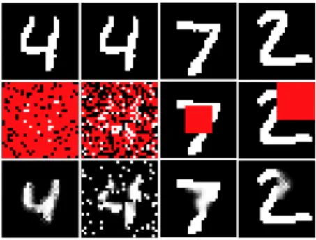
(ii) corrupt(𝑐): Every variable is independently switched, with probability 𝑐, to another value picked uniformly at random, from its discrete support. Then fractional(0.5) is applied to to the data point to obtain the query as in (i). (iii) window(𝑤): [Image only] The center square of width 𝑤 pixels is hidden and those

pixels become query variables, while the pixels around the square are revealed as evidence.

Figure 4-1: In columns 1 to 4, query-creation schemes are: fractional(0.85), corrupt(0.2), window(10) and quadrant(1), respectively (see section 4.1). Original data points on row 1 are converted to queries (Xℰ = 𝑥ℰ, X𝒬, Xℋ) on row 2 (non-red

pixels are observations 𝑥ℰ, red pixels are variables X𝒬 to be guessed). Row 3 shows

marginals guessed by an AGM by plotting 𝑃 (pixel = 1). Note that one AGM was able to answer all of those queries.

those pixels become query variables. The other three quadrants are revealed as evidence.

Some instantiations of these schemes, with specific parameters, on image data, are shown in figure 4-1. We note that the train and test query creation policies do not have to match. In fact, experiment 4.3 is designed to test the failure points of AGMs and EGMs when this mismatch occurs.

Concerning data sets, we use: ten binary data sets used in previous probabilistic modelling work (example: Gens and Pedro [2013]) spanning 16 to 1359 variables. We also use two binarized image data sets (28x28 pixels) which are MNIST [LeCun and Cortes, 2010] with digits 0 to 9 (figure 4-1), and Caltech-101 Silhouettes [Li et al., 2004] (figure 4-2) with shape outlines from 101 different categories.

To show that our method scales to dataset with categorical variables of non-binary support, we created two data sets. First, we use the US Census Data of 1990 (US Census 90), from Dua and Graff [2017] and process the values of every

Table 4.1: Characteristics of the data sets used in our experiments: Name, number of variables, size of discrete support and sizes of the [train, validation, test] splits.

Name |𝒱| |𝒳 | |𝒟train| |𝒟val| |𝒟test|

NLTCS 16 2 16 181 2 157 3 236 Jester 100 2 9 000 1 000 4 116 Netflix 100 2 15 000 2 000 3 000 Accidents 111 2 12 758 1 700 2 551 Mushrooms 112 2 2 000 500 5 624 Adult 123 2 5 000 1 414 26 147 Connect 4 126 2 16 000 4 000 47 557 Pumsb-star 163 2 12 262 1 635 2 452 20 NewsGroup 910 2 11 293 3 764 3 764 Voting 1359 2 1 214 200 350 Pac-NW 169 5 10 000 1 000 5 000 US Census 90 67 7 1 800 000 200 000 450 000 MNIST 784 2 45 000 15 000 10 000 CALTECH 784 2 3 800 300 2 300

variable so that their discrete support is is translated to {0, . . . , 6}. Next, we use the daily precipitation data of the Pacific Northwest from 1949 to 1994 from Widmann and Bretherton [2000]. Stations recording precipitation levels are geographically adjacent to each other and we use the largest possible grid spanning their placements, as shown in figure 4-3, allowing us to treat this data set as image data, as described in experiment 4.2. Here we process precipitation levels so they are all discrete and in the set {1, . . . , 5}.

The sizes of all datasets (train, val, test), together with their corresponding number of variables per data point are shown in table 4.1.

Figure 4-2: The Caltech-101 Silhouettes dataset (CALTECH) has images of the silhouettes of objects from the Caltech-101 dataset, which span 101 categories. Pixels have value 0 or 1, indicating occlusion or not.

Figure 4-3: One data point as an example, from the daily precipitation data of the Pacific Northwest from 1949 to 1994 from Widmann and Bretherton [2000]. Each grid cell is a weather station, which adds one random variable to every data point. The fact that the random variables are regularly organized in euclidean space allows us to experiment with both random and grid graphs in experiment 4.2, for this data set.

4.2

Experiment I: Benchmarking

In this experiment, we train our models on each train data set separately, and test on 1000 unseen points. The inference task fractional(0.7) is used to test every model. Accuracies are given in table 4.2 as the percentage of query variables correctly guessed, over all queries formed from the test set.

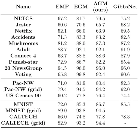
EMP is a baseline graphical model with edge parameters given by empirical probabilities. EGMs train by minimizing the conditional log likelihood score under the inference task given by fractional(0.5). GibbsNet is the deep adversarially trained inference network introduced in section 5. Neural network architectures for the AGM learner and GibbsNet are given in the appendix. By definition, these two models are trained adversarially, in an inference-agnostic fashion. Graph methods (EMP, EGM and AGM) use identical randomized edge sets of size 5|𝒱|. A grid graph structure is also separately experimented with, for image data, as indicated in column 1 of table 4.2.

Results in table 4.2 show that while EGMs are explicitly trained on the fractional task, AGMs are not far behind in performance, and are actually better on all image data sets. GibbsNet being behind AGMs on both image data sets with grid graphs shows the usefulness of the relational inductive bias provided by the graph. GibbsNet is the best performer on image data when its competitors use randomized graphs, as it learns meaningful latent space representations that aid inference through its feed-forward architecture. However once AGMs are equipped with meaningful grid graphs, they get much higher scores on queries on images.

Table 4.2: Performances from experiment I on the fractional(0.7) inference task, across candidate models. Each printed value is an average over 3 trials.

Name EMP EGM AGM

(ours) GibbsNet NLTCS 67.2 81.7 79.5 75.2 Jester 60.6 70.6 65.7 68.2 Netflix 52.1 66.0 63.9 69.5 Accidents 71.3 83.3 83.2 82.5 Mushrooms 81.2 88.0 87.3 87.2 Adult 88.7 92.1 92.1 91.9 Connect 4 63.7 88.8 88.6 87.9 Pumsb-star 72.9 86.7 82.2 85.4 20 NewsGroup 94.5 96.0 96.0 96.0 Voting 65.8 99.8 92.4 90.6 Pac-NW 71.0 81.9 80.4 82.3 Pac-NW (grid) 79.4 94.5 94.2 92.0 US Census 90 60.2 77.8 76.4 74.4 MNIST 72.0 85.3 86.7 85.5 MNIST (grid) 89.0 93.8 94.5 -CALTECH 56.0 74.8 77.8 78.3 CALTECH (grid) 82.9 93.2 94.4

-Along another axis, we benchmark the performance of the AGM model only, with varying ensemble sizes 𝑀 . Essentially, we follow the exact same setup as above for the AGM, except that during inference (section 3), we will separately try values of 𝑀 = 10, 100, 1000, 10000 in an attempt to understand what size of ensemble would give the best results. Results are summarized in the plots of figure 4-4.

At the lowest ensemble size of 𝑀 = 10, performances are much lower than the best performances, and even below chance (50%) in some cases, showing that only 10 models are not enough to form a solid opinion and with such a small population size, the models may even be strongly favoring bad choices. The largest increases in performance were from 𝑀 = 10 to 𝑀 = 100, showing that already at the latter ensemble size, the ensemble effects are much more positive. The best performances are reached in almost every data set at 𝑀 = 1000, barring some exceptions. The increase in performance, from 𝑀 = 100 to 𝑀 = 1000, though smaller than the increase from 𝑀 = 10 to 𝑀 = 100, does not warrant staying at 𝑀 = 100. From 𝑀 = 1000 to 𝑀 = 10000 however, there is practically no increase in performance, but in terms of memory, we are unable to fully parallelize the inference procedure across 10000 models on 1 GPU, forcing us to break the process into several serial steps. 𝑀 = 1000 is the best ensemble size when both performance and practicality are considered. Based on these results, perhaps the most memory-efficient high-performance ensemble size is somewhere between 𝑀 = 100 and 𝑀 = 1000, but 𝑀 = 1000 is memory-efficient enough for us, as data sets of all sizes (table 4.1) are successfully inferred over using only 1 GPU.

Figure 4-4: Inference accuracies (vertical axes) obtained across datasets, using the AGM model (experiment I), where the variable being varied in every plot is the ensemble size 𝑀 (horizontal axes) used during inference. Values used for 𝑀 were 10, 100, 1000, 10000, indicated in logarithm base 10.

4.3

Experiment II: Generalization across inference

tasks on images

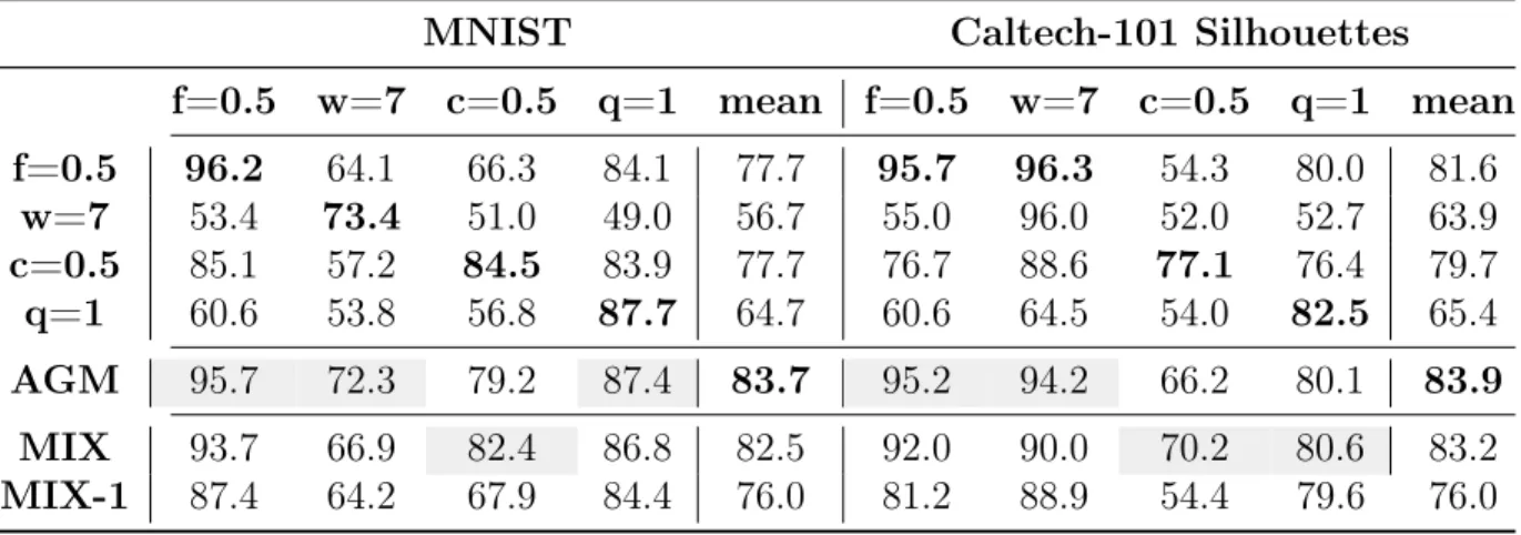
In this experiment, we want to test how well AGMs and EGMs generalize across tasks of varying nature given that experiment 1 employed fractional tasks only. Can AGMs generalize to schemes like corrupt, window and quadrant, despite its inference-agnostic learning style? On the other hand, how widely applicable is an EGM trained using a particular query distribution? In this experiment, we train:

∙ One AGM, adversarially (by definition).

∙ Multiple separate EGMs, on fractional(0.5), window(7), corrupt(0.5) and quadrant(1) tasks respectively.

∙ One mixture EGM (named MIX in table 4.3), by sampling queries successively from the tasks mentioned in the last bullet.

∙ Multiple mixture EGMs (named MIX-1 in table 4.3), which train on a mixture of tasks like MIX, except the specific task they will be evaluated on.

Every model is evaluated on fractional(0.5), window(7), corrupt(0.5) and quadrant(1) tasks. Table 4.3 shows performance of models (trained on tasks shown in the first column, where applicable), and tested on tasks, spread horizontally. From the first four rows (EGMs only), the highest value is mostly on the diagonal as expected when train and test query distributions match. When there is a mismatch, performance levels of EGMs fall drastically in most cases, showing poor generalization. The row for AGMs shows that they come close to the highest EGM score from the first four rows, in every column, showing they generalize well, despite having never explicitly seen these inference tasks. The MIX model (EGM trained on a mixture of the inference tasks) of the last row is the closest competitor to AGMs for generalization. Better performances between the two are indicated by a grey shaded table cell. But even after baking in information about every possible inference task into the MIX training procedure, it surpasses AGMs only in three out of 8 tasks, and has a lower mean score.

The MIX-1 models were included to illustrate the fact that training on a mixture of tasks does not boost the generalization of EGMs to unseen tasks. MIX performed close to AGMs because they were trained on all the evaluation tasks. As soon as a different and completely unseen task is faced (as in the MIX-1 case), the same poor generalization arises.

Another interesting result is that neither training on window(7) itself, nor on a mixture as was done for MIX, constitutes the best way to prepare a model for the window(7) task, in the Caltech-101 case. This shows that it is not always immediately clear, which training task should be picked to prepare for testing on a certain test task, thus requiring experimentation on the part of the practitioner using EGMs.

Table 4.3: Cross-task accuracies (averaged over 3 trials) for EGMs, AGM, MIX and MIX-1. Tasks trained on (where applicable), are in the first column, and test tasks for all models are on the second row. Means of the rows indicate relative generalization abilities.

MNIST Caltech-101 Silhouettes

f=0.5 w=7 c=0.5 q=1 mean f=0.5 w=7 c=0.5 q=1 mean f=0.5 96.2 64.1 66.3 84.1 77.7 95.7 96.3 54.3 80.0 81.6 w=7 53.4 73.4 51.0 49.0 56.7 55.0 96.0 52.0 52.7 63.9 c=0.5 85.1 57.2 84.5 83.9 77.7 76.7 88.6 77.1 76.4 79.7 q=1 60.6 53.8 56.8 87.7 64.7 60.6 64.5 54.0 82.5 65.4 AGM 95.7 72.3 79.2 87.4 83.7 95.2 94.2 66.2 80.1 83.9 MIX 93.7 66.9 82.4 86.8 82.5 92.0 90.0 70.2 80.6 83.2 MIX-1 87.4 64.2 67.9 84.4 76.0 81.2 88.9 54.4 79.6 76.0

4.4

Experiment III: Sampling using AGMs instead

of Gibbs sampling

Motivated by the crisp image samples generated from AGMs and smooth interpolations in latent space (see figure 4-6) (which is an interesting result in itself in the space of discrete GANs, given that CNNs were not included in the architecture), we decided to quantify and compare probabilistic sample quality from AGMs versus from Gibbs samplers defined on EGMs (section 2.1.4). If one wishes to train a graphical model principally for inference, they would have to make a choice between EGMs and AGMs. In this experiment, we show another advantage that comes with using AGMs: the fact that the learner-graphical model pair constitute a sampler that produces high-quality samples in one shot (one pass from 𝑧 to Ψ to 𝑥).

We would like some metric for measuring sample quality and we use the following: given our two samplers, we will use data generated from them, and feed the data to newly-created models for training to solve an inference task, from scratch. The score attained by the new model will indicate the quality of the samples generated by the samplers. Figure 4-7 illustrates this schema.

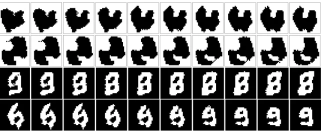
Figure 4-5: Images (column 1) generated from the AGM by providing different random latent vectors 𝑧 to models trained on MNIST (rows 1-2) and Caltech-101 (rows 3-4). Horizontally across every row, the random vectors are gradually changed to a target latent vector. Images are crisp and transition smoothly from source to target.

Figure 4-6: Images sampled from an EGM trained on the fractional(0.5) task through Gibbs sampling involving 10 burn in cycles.

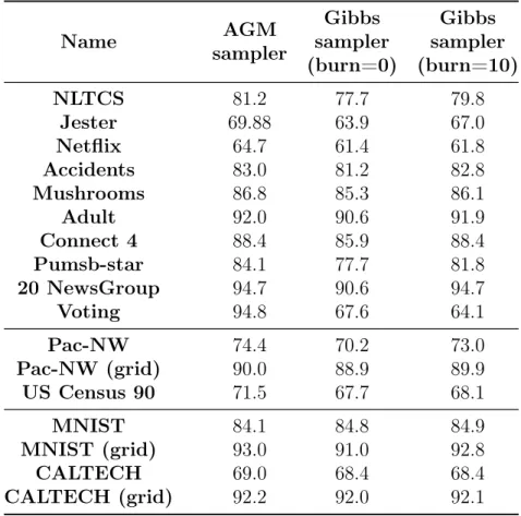
Table 4.4: Inference performances from experiment III, obtained by the EGM eval-uators, trained on data sampled from an AGM sampler, a Gibbs sampler with no burn-in and a Gibbs sampler with burn-in of 10 iterations.

Name AGM sampler Gibbs sampler (burn=0) Gibbs sampler (burn=10) NLTCS 81.2 77.7 79.8 Jester 69.88 63.9 67.0 Netflix 64.7 61.4 61.8 Accidents 83.0 81.2 82.8 Mushrooms 86.8 85.3 86.1 Adult 92.0 90.6 91.9 Connect 4 88.4 85.9 88.4 Pumsb-star 84.1 77.7 81.8 20 NewsGroup 94.7 90.6 94.7 Voting 94.8 67.6 64.1 Pac-NW 74.4 70.2 73.0 Pac-NW (grid) 90.0 88.9 89.9 US Census 90 71.5 67.7 68.1 MNIST 84.1 84.8 84.9 MNIST (grid) 93.0 91.0 92.8 CALTECH 69.0 68.4 68.4 CALTECH (grid) 92.2 92.0 92.1

table 4.1. A is trained adversarially by definition, and B assumes the fractional(0.5) inference task. We generate 1000 samples from each model, and call these sampled data sets 𝑆1 and 𝑆2. If we now train a feshly-created EGM 𝐸1 on 𝑆1 and another

one, 𝐸2 on 𝑆2, from scratch, then test them on the test data set corresponding to

D, then which one out of of 𝐸1 or 𝐸2 has better performance, assuming everything

else about them is identical? If 𝐸1 performs better, then data from A was of better

quality, else, B was the better sampler. The inference task used to test 𝐸1 or 𝐸2 is

Figure 4-7: Schema illustrating the pipeline used in experiment III, with original data from some data set D used to train AGM A and EGM B. Data is separately sampled from both. Each synthetic data set trains a separate EGM (𝐸1 and 𝐸2) from scratch.

These are separately tested on the same test data pertaining to data set D. The key box at the bottom explains the meaning of the different types of arrows used in the schema.

For the Gibbs sampler defined on B, we try two scenarios: one where it uses no burn-in cycles to be similar to the one-shot sampling procedure of A, and one scenario where it has 10 burn-in cycles. Interestingly, as seen in table 4.4, A is better than B regardless of the number of burn-in cycles, bar one exception, and performance when trained on data from A is not that far off the performance from real training data. For B, even 10 burnin steps are not enough for the Markov chain being sampled from, to mix. Since variables have to be sequentially sampled in B, it takes orders of magnitude more time to sample from, compared to sampling from A. The bottleneck in run-time for A is the belief propagation algorithm, but it is parallelizable across edges and can be run entirely using matrix operations [Bixler and Huang, 2018].

In summary, sampling from an AGM is a viable tool and is an added benefit that comes with training AGMs.

Chapter 5

Related Work

Our work combines discrete, undirected graphical models with the GAN framework for training. The graphical model is applied in data space, with the belief propagation algorithm used for inference, over an ensemble of parameterizations. Each parametriza-tion is completely produced by a neural learner essentially allowing our probabilistic graphical model to be parameter-less.

Combining an ensemble of models has been explored in classification [Bahler and Navarro, 2000] and unsupervised learning [Baruque, 2010]. Combined models may each be optimized for a piece of the problem space [Jacobs et al., 1991] or may be competing on the same problem [Freund and Schapire, 1999]. Linear and log-linear ensemble combinations like ours have been analyzed by Fumera and Roli [2005] and the closest work which uses the ensemble approach, by Antonucci et al. [2013], combines Bayesian networks for classification.

The idea of a learner imposing complete sets of parameters onto a parameterless learnee, thus having control over the function expressed by the learnee, has its roots in meta-learning. In Munkhdalai and Yu [2017] one neural network learns to assign weights to another network with the help of memory, and in Bertinetto et al. [2016], a neural network learns to output complete sets of weights for another neural network for one-shot learning to perform classification. Such work involves clever engineering to circumnavigate the issue of explosion in the number of parameters in the learnee as layers of neurons are stacked upon one another, and consequently in the learner

needed to drive the learnee, which often is more heavily parametrized. In our work, the number of parameters in our graphical models (learnees) only increases linearly with the number of edges used (section 3.1). In all experiments, the number of edges varies linearly with the number of random variables being modeled. Hence the neural learner does not have to be too complex as detailed in the appendix.

Using GANs to generate data from discrete distributions is an active area of research, including work of Fathony and Goela [2018], Dong and Yang [2018], and Camino et al. [2018], with applications in health [Choi et al., 2017] and quantum physics [Situ et al., 2018]. Undirected graphical models have been embedded into neural pipelines before. For instance, Zheng et al. [2015] use them as RNNs, Ammar et al. [2014] and Johnson et al. [2016] use them in the neural autoencoder framework, Kuleshov and Ermon [2017] use them in neural variational inference pipelines, and Tompson et al. [2014] combine them with CNNs.

Other works use graph neural networks [Battaglia et al., 2018], but with some connection to classical undirected graphical models. For example, some works learn variants of, or improve on, message passing [Liu and Poulin, 2019, Satorras and Welling, 2020, Gilmer et al., 2017, Satorras et al., 2019]. Other works combine classical graphical models and graph neural networks with one another [Qu et al., 2019], while some use neural networks to replace classical graphical model inference entirely [Yoon et al., 2018, Zhang et al., 2019].

Among the work closest to ours, Fathony et al. [2018] learn tractable graphical models using exact inference through adversarial objectives. Chongxuan et al. [2018] and Karaletsos [2016] use graphical models in adversarial training pipelines, but to model the posterior distribution. GANs have been used with graphs for high-dimensional representation learning [Wang et al., 2017], structure learning [Bojchevski et al., 2018] and classification [Zhong and Li, 2018]. Other relevant GAN works focus on inference in the data space without the undirected graphical structure. For example the conditional GAN [Mirza and Osindero, 2014] and its variants [Xu et al., 2019] allow inference, but conditioned on variables specified during training. [Donahue et al., 2016] and [Dumoulin et al., 2017] introduced the idea of learning the reverse mapping

from data space back to latent space in GANs. GibbsNet [Lamb et al., 2017] is the closest model to ours, though it is not graphical in the data space. GibbsNet allows inference conditioned on any subset of variables, like us. Their inference process is iterative as they transition from data space to latent space and back, stochastically several times, clamping observed values in the process. Our inference mechanism stays within data space, but is also iterative due to the belief propagation algorithm. Each model in our learned ensemble has significantly less parameters than GibbsNet.

Chapter 6

Conclusion

The common approach for training undirected graphical models when the test inference task is known a priori, is empirical risk minimization. In this work, we showed that models produced using this approach (EGMs) fail to generalize across tasks. We introduced an adversarial training framework for undirected graphical models, which instead of producing one model, learns an ensemble of models. Learning an ensemble increases the expressive power of the final model, making up for approximations in inference and model mis-specification. As shown in our experiments, our models (AGMs) generalize over an array of inference tasks, even outperforming EGMs trained on the entire mixture of test inference tasks used. We also showed that AGMs perform comparatively with GibbsNet, which is a deep adversarially learned neural architecture used for inference. Finally, we showed that data can be sampled from AGMs in one shot, which comes as an added benefit of training them for inference tasks. The data produced is of better quality than that produced by a Gibbs sampler defined on an EGM.

Appendix A

Experimental Details

In this section, we present additional information concerning our experiments. All our experiments are run using PyTorch [Paszke et al., 2019] for automatic differentiation, on a Volta 𝑉 100 GPU.

A.1

Architectures:

All architectures are feed forward, consisting of linear layers, with or without Batch Normalization, and with or without Dropout. Activation functions for linear layers are LeakyRelu, Sigmoid or none.

∙ The EGM method has no neural module, all the parameters (edge potentials) are real numbers contained in matrices, with belief propagation implemented entirely through matrix operations (with no iteration over edges), as described in Bixler and Huang [2018].

∙ For the AGM, there are two neural modules: 1. Learner 𝐿𝜃 : R𝑚 → R|𝐸||𝒳 |

2

converting 𝑧 to potentials Ψ:

Linear(in=𝑚, out=2𝑚); Batch Normalization; Leaky ReLU (neg slope 0.1) Linear(in=2𝑚, out=|𝐸||𝒳 |2₎

2. Discriminator 𝐷𝑤 : R𝑁 |𝒳 | → R converting data 𝑥 to Wasserstein-1 distance:

Linear(in=𝑁 |𝒳 |, out=2𝑁 |𝒳 |); Dropout(0.2); Leaky ReLU (neg slope 0.1) Linear(in=2𝑁 |𝒳 |, out=2𝑁 |𝒳 |); Dropout(0.2); Leaky ReLU (neg slope 0.1) Linear(in=2𝑁 |𝒳 |, out=1); Dropout(0.2)

∙ For the GibbsNet baseline, there are three neural modules (note that CNN modules are not used, to keep the architecture identical across image and non-image datasets and to provide a non-relational baseline to compare AGMs to):

1. Decoder 𝐷𝑒𝑐 : R𝑚 → R𝑁 |𝒳 | _{converting 𝑧 to data 𝑥:}

Linear(in=𝑚, out=8𝑚); Batch Normalization; Leaky ReLU (neg slope 0.1) Linear(in=8𝑚, out=8𝑚); Batch Normalization; Leaky ReLU (neg slope 0.1)

Linear(in=8𝑚, out=8𝑚); Batch Normalization; Leaky ReLU (neg slope 0.1)

Linear(in=8𝑚, out=𝑁 |𝒳 |); Sigmoid

2. Encoder 𝐸𝑛𝑐 : R𝑁 |𝒳 | _{→ R}𝑚 _{converting data 𝑥 back to latent vector 𝑧:}

Linear(in=𝑁 |𝒳 |, out=4𝑁 |𝒳 |); Batch Normalization; Leaky ReLU (neg slope 0.1)

Linear(in=4𝑁 |𝒳 |, out=𝑚)

3. Discriminator 𝐷 : R𝑁 |𝒳 |+𝑚 → R converting (data, latent) pairs (𝑥, 𝑧) to Wasserstein-1 distance, in three steps:

(a) 𝐷(𝑎): R𝑁 |𝒳 | → R4𝑁 |𝒳 | converting data 𝑥 to intermediate vector:

Linear(in=𝑁 |𝒳 |, out=4𝑁 |𝒳 |); Dropout(0.2); Leaky ReLU (neg slope 0.1)

(b) 𝐷(𝑏) : R𝑚 → R4𝑚 converting latent vector 𝑧 to intermediate vector:

Linear(in=𝑚, out=4𝑚); Dropout(0.2); Leaky ReLU (neg slope 0.1)

(c) 𝐷(𝑐) : R4𝑁 |𝒳 |+4𝑚 → R converting combination of vectors generated

from data and latent vector, to Wasserstein-1 distance:

Linear(in=4𝑁 |𝒳 | + 4𝑚, out=4𝑁 |𝒳 | + 4𝑚); Dropout(0.2); Leaky ReLU (neg slope 0.1)

Linear(in=4𝑁 |𝒳 | + 4𝑚, out=1)

Note about data (𝑥) being in R𝑁 |𝒳 |:

Instead of using categorical samples as our generated data (obtained from marginal probability distributions 𝜇𝑖, produced for every variable), we follow the WGAN-GP

method [Gulrajani et al., 2017] where the generated data is a concatenation of the marginals in some specific order. This implies that true samples from the train data set also have to be processed into a concatenation of the 𝒳 -dimensional one-hot encodings of the values they propose for every node, to meet the input specifications of the discriminator. This method for discrete GANs is used both for AGMs and GibbsNet in our implementation.

A.2

Hyperparameters:

∙ 𝑧 is sampled from standard multivariate Gaussian 𝒩 (0, 𝐼𝑚), and the

dimension-ality 𝑚 was picked depending on 𝑁 , the number of random variables involved in the data. When 𝑁 is smaller than 500, we use 𝑚 = 64 and otherwise, 𝑚 = 128 is used.

∙ For the ensemble, we used 𝑀 = 1000, where 𝑀 is the number of models used for the pooling mechanism seen in equation 3.6.

∙ In both the EGM and AGM, we need to carry out belief propagation. The number of steps of belief propagation was kept constant and was 25 in EGM, 5 in AGM. These numbers gave the best results for their respective models. ∙ For the AGM method, 𝜆 = 10 was used for the coefficient of the regularization

term of equation 3.4.

∙ Also, our implementation of the WGAN-GP method for adversarial training, the discriminator is trained for 10 steps, for every update step on the generator. ∙ The learning rates are 1𝑒 − 2 for EGM (matrix of parameters) and 1𝑒 − 4 for

the AGM (learner and discriminator).

∙ We used 500 and 3000 training gradient descent steps enough across data sets to train the EGMs and AGMs respectively.

∙ The batch sizes used were 128 for training both AGM and EGM, and for testing the AGM, with 𝑀 = 1000, the batch sizes used were reduced to 16.

Bibliography

Waleed Ammar, Chris Dyer, and Noah A. Smith. Conditional random field autoen-coders for unsupervised structured prediction. CoRR, abs/1411.1147, 2014. URL http://arxiv.org/abs/1411.1147.

Alessandro Antonucci, Giorgio Corani, Denis Deratani Mauá, and Sandra Gabaglio. An ensemble of bayesian networks for multilabel classification. In Twenty-Third International Joint Conference on Artificial Intelligence, 2013.

Dennis Bahler and Laura Navarro. Methods for combining heterogeneous sets of classifiers, 2000.

B. Baruque. Fusion Methods for Unsupervised Learning Ensembles. Studies in Computational Intelligence. Springer Berlin Heidelberg, 2010. ISBN 9783642162046. URL https://books.google.com/books?id=oVGnmPTOI48C.

Peter W. Battaglia, Jessica B. Hamrick, Victor Bapst, Alvaro Sanchez-Gonzalez, Vinícius Flores Zambaldi, Mateusz Malinowski, Andrea Tacchetti, David Raposo, Adam Santoro, Ryan Faulkner, Çaglar Gülçehre, H. Francis Song, Andrew J. Ballard, Justin Gilmer, George E. Dahl, Ashish Vaswani, Kelsey R. Allen, Charles Nash, Victoria Langston, Chris Dyer, Nicolas Heess, Daan Wierstra, Pushmeet Kohli, Matthew Botvinick, Oriol Vinyals, Yujia Li, and Razvan Pascanu. Relational inductive biases, deep learning, and graph networks. CoRR, abs/1806.01261, 2018. URL http://arxiv.org/abs/1806.01261.

Luca Bertinetto, João F. Henriques, Jack Valmadre, Philip H. S. Torr, and Andrea Vedaldi. Learning feed-forward one-shot learners. CoRR, abs/1606.05233, 2016. URL http://arxiv.org/abs/1606.05233.

Reid Bixler and Bert Huang. Sparse-matrix belief propagation. In UAI, 2018.

Aleksandar Bojchevski, Oleksandr Shchur, Daniel Zügner, and Stephan Günnemann. Netgan: Generating graphs via random walks. In ICML, 2018.

Jörg Bornschein and Yoshua Bengio. Reweighted wake-sleep. CoRR, abs/1406.2751, 2014.

Ramiro Camino, Christian A. Hammerschmidt, and Radu State. Generating multi-categorical samples with generative adversarial networks. ArXiv, abs/1807.01202, 2018.