Comparing Learning Techniques for Hidden Markov
Models of Human Supervisory Control Behavior
The MIT Faculty has made this article openly available.
Please share
how this access benefits you. Your story matters.
Citation
Boussemart, Yves et al. "Comparing Learning Techniques
for Hidden Markov Models of Human Supervisory Control
Behavior." AIAA Infotech@Aerospace'09 Conference and AIAA
Unmanned...Unlimited Conference, 6-9 April 2009, Seattle,
Washington.
As Published
http://www.aiaa.org/agenda.cfm?
lumeetingid=2070&viewcon=agenda&pageview=2&programSeeview=1&dateget=07-Apr-09&formatview=3
Publisher
American Institute of Aeronautics and Astronautics
Version
Original manuscript
Citable link
http://hdl.handle.net/1721.1/56295
Terms of Use
Attribution-Noncommercial-Share Alike 3.0 Unported
1
Comparing Learning Techniques for Hidden Markov
Models of Human Supervisory Control Behavior
Yves Boussemart*, Jonathan Las Fargeas†, Mary .L. Cummings‡, and Nicholas Roy§
Humans and Automation Lab, Massachusetts Institute of Technology, Cambridge, MA, 02139
Models of human behaviors have been built using many different frameworks. In this paper, we make use of Hidden Markov Models (HMMs) applied to human supervisory control behaviors. More specifically, we model the behavior of an operator of multiple heterogeneous unmanned vehicle systems. The HMM framework allows the inference of higher operator cognitive states from observable operator interaction with a computer interface. For example, a sequence of operator actions can be used to compute a probability distribution of possible operator states. Such models are capable of detecting deviations from expected operator behavior as learned by the model. The difficulty with parametric inference models such as HMMs is that a large number of parameters must either be specified by hand or learned from example data. We compare the behavioral models obtained with two different supervised learning techniques and an unsupervised HMM training technique. The results suggest that the best models of human supervisory control behavior are obtained through unsupervised learning.
Nomenclature
= Probability of going from state i to state j = Maximum likelihood estimate of
A = State transition matrix
= Probability of observing symbol c in state i = Maximum likelihood estimate of
= Observable emission matrix
H = Hidden Markov Model
= Length of observation sequence s
M = Number of observable symbols
N = Number of hidden states = t-th observation in sequence s
= Set of possible hidden states = Property of being at state i at time t
V = Set of possible observables
= Forward probability = Backward probability = Viterbi backtrack pointer
= Probability of the observation sequence and that the state at time t is i
= Likelihood of model H
= Initial probability of being in state i = Initial probability vector
= Probability of the observation sequence and that the state at time t and t+1 are i and j = Smoothed estimator for
= Learning rate for all ’s = Learning rate for all ’s = Smoothed estimator for
I. Introduction
ehavioral models of human operators engaged in complex, automation-mediated high-risk domains, such as those typical in human supervisory control (HSC) settings, are of great value because of the high cost of operator failure1. Although generic models of full human behaviors are intractable, smaller scale models of behaviors in specific contexts are desirable both to predict possible system failures in various modes of operation, as well as to predict the impact of design interventions. While many techniques have been used to model different aspects of human behavior2, 3, partially observable models such as Hidden Markov Models (HMM) have been shown to be a good fit for modeling unobservable operator states4, 5. In this paper we concentrate on HMMs applied to the
* Ph.D. Candidate, Engineering Systems Division, 77 Mass. Ave. 33-407, Cambridge MA, 02139
† B.Eng. Candidate, Dept. of Aeronautics and Astronautics, 77 Mass. Ave. 33-407, Cambridge MA, 02139 ‡
Associate Professor, Dept. of Aeronautics and Astronautics, 77 Mass. Ave. 33-311, Cambridge MA, 02139, Associate Fellow
§ Assistant Professor, Computer Science and Artificial Intelligence Lab, 77 Mass. Ave. 33-315, Cambridge MA, 02139
human supervisory control context. HMMs are stochastic models of time series processes mainly used for the modeling and prediction of sequences of symbols. In the HSC context, HMMs can be used to recognize and predict human operator behavior, given some level of intermittent interaction with an automated system6.
One difficulty in using HMMs to model any real world process is that the model is parametric; any HMM inference algorithm requires an a priori description of the likelihood of specific observations and the likelihood of state changes. These parameters can be specified according to domain knowledge, or acquired from training data in a “model learning” process. For example, Bayesian model learning computes model parameters so as to maximize the likelihood of the model given a training data set. The learning algorithms can either be unsupervised or supervised. While an unsupervised learning algorithm only makes use of the information contained in the training data set to extract the optimal set of model parameters, supervised learning methods require that the data is augmented with a priori information, or labels, in order to guide the learning process. The labels usually consist of input data associated with the expected model output, defined by a subject matter expert. The supervised methodology has been favored by the machine learning community in the past for two reasons: (1) the simplest supervised learning methods offer better computational efficiency compared to unsupervised learning methods, and (2) the labels in the training data are assumed to be derived from reliable ground-truth, thereby increasing the amount of information captured in the model. Our focus in this paper is on operator models of human behavior and, in this context, we argue that it is fundamentally impossible to correctly label the training data because operator cognitive states are not observable. Without ground-truth, we hypothesize that human bias7, 8 is unavoidably introduced into the training data labels, which greatly influences the learning process, and may generate uninformative or incorrect models.
In order to support our hypothesis, we define the HMM formalism along with the mathematical description of three learning techniques we compare: (1) purely supervised learning9, (2) unsupervised learning9 and (3) smooth supervised learning10. We then introduce the data set used to train the models, present the results and finally offer our conclusions on the respective values of the different techniques.
II. Hidden Markov Models
A. Formal Definition
HMMs were first formally defined by Baum et al.11 and their application was popularized by Rabiner et al.9 HMMs have since then been used in a large number of different contexts and have proven valuable in diverse fields such as speech recognition12, financial data prediction13, signal processing14, and generic temporal data clustering15. HMMs consist of stochastic Markov chains based around a set of hidden states whose value cannot be directly observed. Each hidden state generates an observable symbol according to a specific emission function. Although the sequence of hidden states cannot be observed directly, the probability of being in a specific state can be inferred from the sequence of observed symbols. Transition functions describe the dynamics of the hidden state space. There are thus two types of probability parameters: the state transition probabilities and observable symbol output probabilities. Given a finite sequence of hidden states, all the possible transition probabilities and symbol output probabilities can be multiplied at each transition to calculate the overall likelihood of all the output symbols produced in the transition path up to that point. Summing all such transition paths, one can then compute the likelihood that the sequence was generated by the HMM.
Adopting the classic notation from Rabiner et al.9, let N be the number of states in the HMM and M be the number of observation symbols (i.e. the dictionary size). Let denote the property of being in state at time . The state transition probability from state to state is where
The symbol output probability function in state i is , where . The model parameters must be valid probabilities and thus satisfy the constraints:
(1)
The initial probability of being in state at time is where . Thus, an HMM is formally defined as the tuple: . Figure 1 illustrates the HMM concept by showing a graphical representation of a 3-state model, where the set of hidden states’ transition probabilities are defined as a
3
Fig. 1. A Three-state Hidden Markov Model.
An HMM is said to respect the first order Markov assumption if the transition from the current state to the next state
only depends on the current state such that .
Three main computational issues need to be addressed with HMMs: model evaluation, most likely state path, and model learning. The first issue is the evaluation problem, i.e. the probability that a given sequence is produced by the model. This value is useful because, according to Bayes’ rule, it is a proxy for the probability of the model given the data presented. We can thus compare different models and choose the most likely one by solving the evaluation problem. The evaluation problem is solved with the forward/backward dynamic programming algorithm. Let the be the sth training sequence of length , and the tth symbol of be , so that . We can define the forward probability as the probability that the partial observable sequence is generated and that the state at time t is j. The forward probability can be recursively computed by the following method:
(2)
where if j can be the first state and otherwise.
Similarly, we can define the backward probability as the probability of the partial observable sequence and that the state at time t is i. The backward probability can also be recursively computed as follows:
(3)
where if i can be the last state and otherwise.
We can now compute the likelihood that the given training sequence is generated by HMM and solve the state evaluation problem:
The second issue consists of determining the most probable (“correct”) path of hidden states given a sequence of observables: the most common way to solve this problem is by the Viterbi algorithm16. The Viterbi algorithm is a dynamic programming algorithm that finds the most probable sequence of states given
by using a forward-backward algorithm across the trellis of hidden states. More specifically, let be the highest probability path across all states which ends at state i at time t:
(5)
The Viterbi algorithm finds the maximum value of iteratively, and then uses a backtracking process to decode the sequence of hidden states taken along the path of maximum likelihood
Finally the last problem is the learning of the model, which is, given a sequence of observable, what is the maximum likelihood HMM that could produce this string? The different solutions to this problem are described in the next section.
B. Learning Strategies for Hidden Markov Models
HMMs are useful for modeling sequences of data because their structure provides inferences over unobservable states. The parameters of an HMM , i.e. the characteristics of the sequences of data being modeled, are trained to maximize , the sum of the posterior log-likelihoods of each training sequence . Conceptually, the easiest way to model data is to start from known examples and associated model states. Provided that a large enough corpus of annotated data (pairs of input and desired output) is available, different supervised learning techniques can be used to estimate the parameters of the HMM. However, if no annotated data is available, it is still possible to automatically derive the probabilistically optimal parameters of the HMM model. This case corresponds to unsupervised learning.
For ease of notation, we introduce as the probability that the sequence is generated by the HMM and that the state at time t is i. We also define as the probability that the sequence is generated by the HMM and that the state at time t and t+1 are i and j respectively:
(6)
(7)
Classic Supervised Learning
Classic supervised learning is the simplest way to extract model parameters from labeled data. In essence, the idea is to maximize the probability of the observations.
Let us again assume that our training data consists of sequence of observations . It can be shown that the Most Likely Estimate (MLE) of emission probability distribution given the training data is distributed according to the frequency of emissions in the data. We can calculate the frequency by counting how often an observation was generated by a state. Similarly, the most likely transition distribution given the data is distributed according to the frequency of transition from one state to another in the data. Ordinarily, we cannot count the frequency of state transitions or observation emissions from a particular state because the state is hidden. However, supervised learning makes the assumption that during training, we have access to the underlying state sequence and can therefore “label” each observation in with the corresponding true, hidden state. The transition matrix of can therefore be computed directly by counting the relative frequency of the transition between all states i and j. Similarly, the emission functions can be computed by counting the number of times a specific observation c has been observed given a state j. More formally, if we define as the number of time state follows state and as the number of time state j is paired with emission c:
5
(9)
The MLE estimates of then are:
(10)
Similarly, the MLE estimates of are:
(11)
Using this supervised learning technique to compute the HMM model parameters is very simple and runs in , where is the length of a sequence.
Unsupervised Learning
It may be, however, that even during training it is not feasible to have access to the underlying hidden state. Without this label, we cannot use the above algorithm because when counting state transitions, we no longer know which state transitioned to where at each time step and we no longer know which state to assign credit for each observation. We can, however, use unsupervised learning algorithms to not only infer the labels but also infer the model during training. The most commonly used algorithm for HMMs is a form of Expectation-Maximization (EM) called the Baum-Welch algorithm. Just as in supervised learning, the goal of the Baum-Welch algorithm is to maximize the posterior likelihood of the observed sequence for a given HMM. More formally, Baum-Welch computes the optimal model such that:
(12)
We cannot, however, use equations (10) and (11) directly because we do not know the state at each time step t. EM operates by hypothesizing an initial, arbitrary set of model parameters. These model parameters are then used to estimate a possible state sequence via the Viterbi algorithm. This is the expectation or E-Step of the EM algorithm. The model parameters are then re-estimated using equations (10) and (11) given the state labels . This is the maximization or M-Step of the EM algorithm. We could make the assumption that the state sequence is correct; however, the state sequence can be very uncertain in cases, and assuming that the state sequence is correct is likely to lead to failures in determining the model parameters. The EM algorithm takes the uncertainty of the state sequence estimate into account by using the probability of being in state at time t to estimate transition and emission probabilities. The probability is re-estimated using and based not on the frequency of state transitions from i to j in the data, but on the likelihood of being in state i at time t and the likelihood of being in state
j at time t+1. Note that our frequencies or counts in equations (10) and (11) are not integer counts but likelihoods
and are therefore fractional. Similarly, is re-estimated with as the likelihood of being in state i when the observation was c. The equations of re-estimation are:
(13)
(14)
Through this iterative procedure, it can be proven that the Baum-Welch algorithm converges to a local optimum. The process described above assumes that the model structure (i.e. the number of hidden states) is known in advance. In most practical settings, this assumption is unrealistic and the structure of the model must be determined through a process called model selection. While there are many different criteria used to determine the validity of a model, we adopt in this work an information-theoretic metric called the Bayesian Information Criterion17 (BIC).
This metric allows the comparison of different models, in particular with different number of hidden states, trained on the same underlying data. The BIC penalizes the likelihood of the model by a complexity factor proportional to the number of parameters P in the model and the number of training observations K.
(15)
Smooth Supervised Learning
Smooth supervised learning was first introduced by Baldi et al.18 in order to avoid issues with sudden jumps or absorbing probabilities of 0 during the parameter update process. The absorption property of null probabilities is an issue because once a transition or emission function is set to 0, it cannot be used again. The idea for the supervised case is to minimize the distance between the a-priori labels and the labels estimated as most likely by the HMM. This algorithm can be tailored for sequence discrimination10, and we can replace the usual and with real-value parameters and defined as (with being a constant):
(16)
Let be the target value of the likelihood of the pre-labeled observations and associated symbols given the HMM H. The probability will depend on the length of the sequence, so we introduce which scales the probability with respect to the length of the sequence. and are constants that normalize for different observation sequence sizes:
(17)
The algorithm thus tries to maximize in order to maximize the fit of the model to the data. Given and as learning rates, the update rules for and are as follows:
(18)
In order to reach convergence, the constants and learning rates need to be changed for each new training set. Because the solution space is highly-non-linear there is no analytical method to choose these parameters appropriately; hence the constants and rates have to be found by a very time-consuming process of trial and error to maximize the model likelihood.
C. Hidden Markov Models of Human Supervisory Control Behavior
We posit that the dual-chained structure of HMMs is well suited to modeling human behavior in a supervisory control system. HMMs are appropriate because while the operator cognitive states are not directly observable, they can be inferred from his or her actions. This is similar to the HMM notion of hidden states that must be inferred from observable symbols. Thus, we liken the hidden states of the HMM to the unobservable operator states that must be inferred from directly observable behaviors such as user interface interactions. Based on similar premises, some researchers have used HMMs to model human attention allocation based on eye-tracking data4. In contrast, we use HMMs in order to detect patterns in user behavior based on user interface events which constitute the observable symbols. The hidden states then can be seen as higher cognitive states or intent that gave rise to the pattern of observable actions. For example, a controller selecting an unmanned vehicle (UV) would be an observable symbol, whereas his intention to replan the UV’s goal would be a hidden operator state.
7
III. Experiment and Results
A. RESCHU
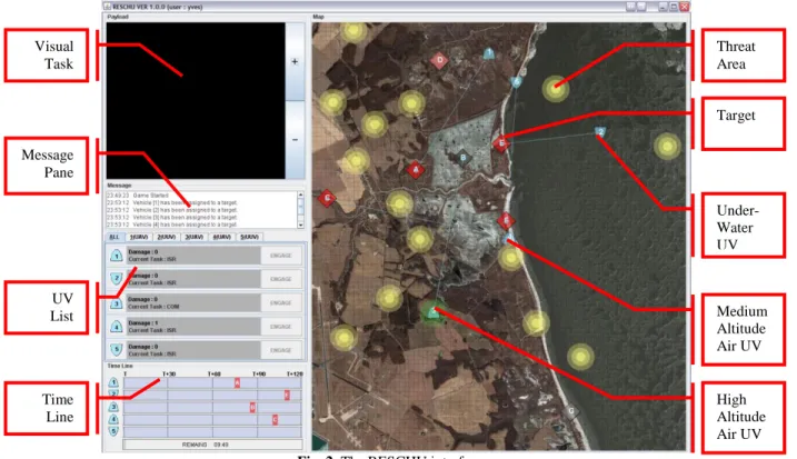
Data used to develop the HMM of a human supervisory control system, specifically that of a single operator controlling multiple unmanned vehicles, was obtained from the experiment described in Nehme et al19. While the goal of the original experiment was to validate a discrete event simulation of an operator controlling multiple heterogeneous unmanned vehicles, the recorded user interface interactions represent a rich corpus of supervisory control behavior. In the experiment, the Research Environment for Supervisory Control of Heterogeneous Unmanned Vehicles (RESCHU) simulator was used to allow a single human operator to control a team of UVs composed of unmanned air and underwater vehicles (UAVs and UUVs) (Figure 2).
Fig. 2. The RESCHU interface
In RESCHU, the UVs perform surveillance tasks with the ultimate goal of locating specific objects of interest in urban coastal and inland settings. UAVs can be of two types: one that provides high level sensor coverage (High Altitude Long Endurance or HALEs, akin to Global Hawk UAVs), while the other provides more low-level target surveillance and video gathering (Medium Altitude Long Endurance or MALEs, similar to Predator UAVs). In contrast, UUVs are all of the same type. Thus, the single operator controls a heterogeneous team of UVs which may consist of up to three different types of platforms, each with different characteristics.
In the rules of this simulation, the HALE performs a target designation task (simulating some off-board identification process). Once designated, either MALEs or UUVs perform a visual target acquisition task, which consists of looking for a particular item in an image by panning and zooming the camera view. Once a UV has visually identified a target, an automated planner chooses the next target assignment, creating possibly sub-optimal target assignments that the human operator can correct. Furthermore, threat areas appear dynamically on the map, and entering such an area could damage the UV, so the operator can optimize the path of the UVs by assigning a different goal to a UV or by adding waypoints to a UV path in order to avoid threat areas.
Participants maximized their score by 1) avoiding threat areas that dynamically changed, 2) completing as many of the visual tasks correctly, 3) taking advantage of re-planning when possible to minimize vehicle travel times between targets, and 4) ensuring a vehicle was always assigned to a target whenever possible. Training was done through an interactive tutorial and an open-ended practice session. After participants felt comfortable with the task and the interface, they started a ten minute experimental session. After completing the experiment, the participants could see their score which corresponded to the total number of targets correctly identified. All data were recorded
Visual Task Message Pane UV List Time Line Target Threat Area Under- Water UV Medium Altitude Air UV High Altitude Air UV
to an online database. The data of interest for this project consisted of user interactions with the interface in the manner of clicks, such as UV selections on the map or on the left sidebar, waypoint operations (add, move, delete) goal changes, and the start and end of visual tasks.
Data was collected on 49 subjects via the experimental procedure described above. The data collected amounts to about 8 hours of raw experimental data and about 3500 behavioral sample points. The average length for each sequence consisted of about 71 user interface events.
B. Applying Hidden Markov Models to Human Supervisory Controller Behavior
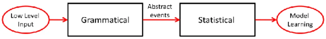
Determining the parameters of a Hidden Markov Model of user behavior requires training the model on the observed behavioral data. The raw behavioral data, which consists of the logged user interface events described above, cannot be used directly by the HMM learning algorithms, and must be pre-processed. Figure 3 shows this process, which consists of a grammatical and a statistical phase.
Fig. 3. A combined grammatical and statistical approach is used to infer future behavior from a stream of current behavior.
First, in the grammatical phase, low level input data (the logged events) are translated into abstract events by the use of a syntactic parser. The grammatical rules were established through a cognitive task analysis20(CTA) that highlighted the important interactions of the operator with the interface. The goal of the CTA was to define clusters of events that are similar in the cognitive sense. In particular, the CTA focused on the formal elicitation of (1) the information required for each operation, (2) the result of each operation and (3) the objective function used to evaluate the outcome of the actions. The resulting grammatical space is shown in Table 1. User interactions were first discriminated based on the type of UV under controlled. This is the y-axis of the grammar. Then, the interactions with each of the UV types were separated into different modes: selection on either the sidebar or on the map, waypoint manipulation (addition, deletion and modification), goal changes, and finally, the visual task engagement. This is the x-axis of the grammar. The sequences of low-level user interactions were thus translated into a sequence of integers suitable for the statistical phase.
Table 1. The RESCHU grammar.
All Underwater UV
Aerial UV High Altitude UV
UV Type / Mode Select Sidebar Select Map Waypoint Edit Waypoint Add/Del Goal Visual Task/Engage
The second step of the process is the statistical learning phase which tries to model this time sequence of data. During this phase, the HMM parameters are trained using sequences of either labeled or unlabeled data. The initial HMM parameters were randomly chosen. In this experiment, we used 49 data traces of individual user trials, and we used a 3-fold cross-validation by training the algorithm on 46 subjects and keeping 3 subjects as a test set. This procedure was repeated multiple times in order to ensure the learning process was not over-fitting the data.
C. State Labeling
For the HMM leveraging supervised learning, labels are needed. However, due to the futuristic nature of the single operator-multiple unmanned vehicle system, no subject matter expert is available to label the data by hand. Through the cognitive task analysis, we derived an initial set of labels that were known to be recurrent. This set of patterns was iteratively re-defined by a Subject Matter Expert in order to increase the proportion of labeled states. Without a more principled way to determine the internal state of each operator, the task analysis suggested that certain sequences of user-interface interactions could be grouped as clusters or states. For example, a common task for an operator is to replan the path of a UV and the CTA allowed us to determine the necessary steps to perform that task. The a priori labels consisted of:
9
2. Monitoring: interaction with the UVs based on selection on the sidebar or the map 3. Visual Task: set of action that results in the visual/engage action
4. Preemptive Threat Navigation: adding a series of waypoints in order to simplify changing the course of the vehicle should the need arise.
This labeling scheme allowed us to cover about 80% of the training sequences and any observable that did not get labeled was dropped from the training set. These labels align with those basic underlying operator functions that form the core of supervisory control of unmanned vehicles which include navigation, vehicle health and status monitoring, and payload management21 (which in this case is the visual task.)
D. Classic Supervised Model
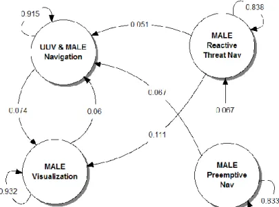
The model below represents the HMM obtained with the classic supervised learning method. All transitions with a weight under 5% are not drawn for legibility purposes. In general, the supervised learning algorithms find the optimal set of parameters for state transitions and the emission functions. Models can contain four states which may correspond to any type of interaction as defined by the a-priori patterns along with a specific category of UV or UVs that is the most likely to have produced the observable. The annotated arrows between the states represent the probability of going from one state to another. The emission functions are not represented explicitly but are encapsulated in the hidden state labeling. With the RESCHU data set, the obtained model shows that given the subject-matter expert-defined states, operator interactions with the HALEs do not appear as a distinct state. While operators interacted with the HALEs less than they did with the MALE UAVs and the UUVs, because there was a clear pattern in the use of a HALE prior to use of a MALE for unknown targets, we anticipated that this would be a state with a clearly assigned meaning.
Fig. 4. Model of a human operator of multiple unmanned systems obtained with classic supervised learning
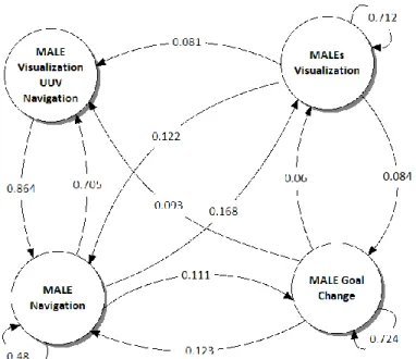
E. Smooth-Supervised Models
The model in Fig. 5 represents the model obtained with the smooth supervised learning method. Again, all transitions with a weight under 5% are not drawn for legibility purposes. The model obtained is different from the one obtained through classic supervised learning. While the transition probabilities between hidden states as less deterministic (as indicated by the higher number of likely transitions between hidden states), operator interaction with the HALEs again disappear and do not appear as a state as defined by the learning algorithm.
.
Fig. 5. Model of a human operator of multiple unmanned systems obtained with smooth supervised learning
F. Unsupervised Models
Because there is no prior knowledge assumed about the model structure, the unsupervised method first requires performing model selection in order to determine how many hidden states the model should have. Models with a number of hidden states ranging from 2 to 15 were trained multiple times with different randomly assigned initial parameters in order to avoid convergence to a local optimum. The training was performed through the unsupervised Baum-Welch learning technique. The BIC for each model was computed and 4-state models appeared to be the most adequate models structure. Figure 6 represents the model obtained by the process described above. Again, all transitions with a weight under 5% are not drawn for legibility purposes. This model is markedly different from the models obtained with the supervised learning techniques, most notably in that the HALE and UUV interactions are grouped together in a clearly distinct state. This denotes that the unsupervised model was able to recognize the much less frequent interactions with UUVs and HALEs as different from that with the MALEs.
Fig. 6. Model of a human operator of multiple unmanned systems obtained with unsupervised learning
IV. Discussion and Model Comparisons
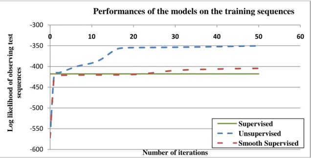
Given the three different models, it is interesting to consider how fast the training converges to a stable set of parameters, and how good the data fit the models after the training process. Figure 7 shows the evolution of the three learning techniques over the course of 50 learning iterations.
11
Fig. 7. Model fit in terms of test set likelihood for the three different training techniques
The first thing to note is that, as expected, the supervised algorithm converges in the first iteration and provides a constant performance baseline. The first few iterations of the smooth supervised algorithm, conversely, are quite poor. However, at the 25th iteration, the smooth supervised model surpasses the classic supervised model and plateaus at around the 30th iteration. The first few learning iterations of the unsupervised model behave very closely to the smooth supervised. After the 3rd iteration, however, while the smooth supervised model plateaus for the first time, the unsupervised algorithm log likelihood continues to increase and converges at the 20th learning iteration. In terms of log likelihood, the performance differences are clear: the unsupervised learning method gives rise to a model that is more likely than both supervised methods. The smooth supervised model provides slightly superior posterior log likelihood than the classic supervised one.
Adopting a human-centric point of view, it is interesting to compare how much human effort was required to generate the above models. For both supervised methods, the cost of labeling the data was quite high as our initial undertaking was to execute a cognitive task analysis of the single operator - multiple unmanned systems in order to define a likely set of behaviors. Cognitive task analyses are labor intensive and are somewhat subjective, so there is no guarantee that the outcome behaviors are correctly identified.
Moreover these a priori defined patterns then had to be tagged in all the sequences in order to construct the corpus of training and testing data. In order to avoid the known risks of human judgment bias22in the state definition process, an iterative approach was adopted in which multiple acceptable sets of state definitions were compared to the data. The set of definitions that provided the better explanation for the states was then chosen. It is important to note that expert knowledge of the task was required in all phases of this lengthy process. Thus, in addition to being extremely time-intensive, it is recognized that expert labeling is a costly and sometimes subjective process that can unnecessarily constrain the resulting models to the types of behaviors seen as important by human experts5.
The classic supervised algorithm was straight-forward to execute and, by design, converged in one single iteration. In the case of the smooth supervised algorithm, however, we had to spend a considerable amount of effort tweaking the learning parameters and the different constants in the error distance function in order to achieve a reasonable convergence point. Unfortunately, due to the highly non-linear features of the solution space, it was impossible to use standard optimization algorithms such as grid-based exploration or sequential quadratic programming (SQP). Our approach then was to use a process similar to simulated annealing in which we initially chose a large number of random algorithm parameter values and focused the exploration around the most “promising” initial points, where promising was measured as the closeness between the expected and modeled distance in label-space. Finally, the Baum-Welch (unsupervised) method required some effort coding but subsequently did not require human intervention to reach convergence.
-600 -550 -500 -450 -400 -350 -300 0 10 20 30 40 50 60 L o g lik eliho o d o f o bs er v ing t est sequences Number of iterations
Performances of the models on the training sequences
Supervised Unsupervised Smooth Supervised
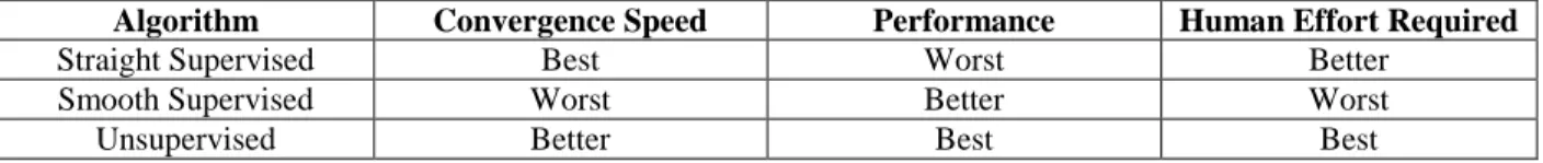
Table 2. Qualitative performance summary of the learning algorithms.
Algorithm Convergence Speed Performance Human Effort Required
Straight Supervised Best Worst Better
Smooth Supervised Worst Better Worst
Unsupervised Better Best Best
Table 2 shows a qualitative summary of the arguments presented above. We suggest that even when experts are available to decide which operator states should be labeled, uncertainty and subjective judgment cannot be eliminated from the process. Furthermore, even with a defined state space of labels, it is not possible for an expert to look at the data and unambiguously assign labels to observable states. This is especially true for states with no clear ground truth. The possible bias introduced in the labeling process is detrimental to the fit and therefore the predictive ability of the model obtained through supervised learning. Therefore, we submit that unsupervised methods should be preferred to the supervised technique in modeling human interactions with automated systems.
In addition to the quantitative metrics such as convergence speed and performance, it is interesting to analyze the models for the explanatory mechanism they can provide. For the supervised models, the results obtained are similar in that they overtly emphasize the role of the MALEs and UUVs. Both supervised models, based on the human-biased grammar, disregard a major part of the problem space: the existence of a 3rd vehicle category (the HALEs). The unsupervised learning technique, on the contrary, segregated the HALE and UUV interactions in a separate state. The unsupervised technique also detected that there were very few marine targets, and thus the majority of the interactions with UUVs were spent in target visual task and not replanning. Such examples show the richness of the interpretation that can be obtained from analyzing a non-biased model that is based on statistical properties of operator interactions. The unsupervised model can thus be used as an exploratory tool for the human behaviors, which could be useful for design, training and monitoring of unmanned vehicle supervisory control systems.
Analyses, both quantitative (i.e. model likelihood) and qualitative (i.e. model interpretation), indicate that for the purpose of modeling HSC operator states, the use of supervised learning is inherently flawed. The results we obtained showed that the supervised models yielded not only poorer prediction rates, but also failed to capture important characteristics of operator behavior. The poor results could be blamed, quite rightly, to poor a priori labeling of the states, and that the results could have been very different with better labeling. While we agree, this again highlights the subjective nature of expert state labeling in the presence of uncertainty. In the specific context of human supervisory control modeling, we argue that it is very difficult, if not impossible, to obtain a correct set of labels. Even using multiple experts to label in hopes of reducing the negative impact of imperfect labeling is not guaranteed to lead to better results23.
The nature of correct -or even close enough- labels is very domain specific, and when modeling high-risk systems such as those in command and control systems, we propose that the more conservative and objective unsupervised approach is superior. Application of supervised learning methods to domains with known ground truth and objective label identification, such as determining facial expressions24 or melodic content25 do not suffer from these limitations. However, our results demonstrate that the lack of known ground-truth to annotate operator states leads to poor models, and that unsupervised learning should be strongly considered for future work in similar contexts.
V. Conclusion
In this paper we compared models of human supervisory control obtained through supervised learning and unsupervised learning. Our results suggest that not only do the supervised learning methods require significantly more human involvement both in terms of state labeling and parameter adjustments, they also tend to perform worse than the models obtained with unsupervised learning. The lack of accessible ground truth to label operator cognitive states and inherent human decision making biases in labeling hinders the supervised learning of operator models. Although domain specific, we propose that operator modeling efforts could greatly benefit from using unsupervised learning techniques.
Acknowledgments
13
References
1 N. G. Leveson, "Software Safety: Why, What, and How" (1986) 18 Computing Surveys 125-163.
2 D. G. Wayne, E. J. Bonnie and E. A. Michael, The precis of Project Ernestine or an overview of a validation of GOMS,
Proceedings of the SIGCHI conference on Human factors in computing systems, (Monterey, California, United States 1992).
3 J. Anderson, Rules of the Mind, (Hillsdale, New Jersey 1993).
4 M. Hayashi, Hidden Markov Models to Identify Pilot Instrument Scanning and Attention Patterns, IEEE International
Conference on Man and Cybernetics, vol. 3, (2003), pp. 2889-2896.
5 J. Hoey, "Value-Directed Human Behavior Analysis from Video Using Partially Observable Markov Decision Processes" (2007) 29 IEEE Trans. Pattern Anal. Mach. Intell. 1118-1132.
6 Y. Boussemart and M. L. Cummings, Behavioral Recognition and Prediction of an Operator Supervising Multiple Heterogeneous Unmanned Vehicles, In G. Coppin (ed.), Humans Operating Unmanned Systems, HUMOUS'08, (Brest, France 2008).
7 D. Kahneman and A. Tversky, "Prospect Theory: An Analysis of Decision under Risk" (1979) 47 Econometrica 263-292. 8 A. Tversky and D. Kahneman, "Judgement Under Uncertainty: Heuristics and Biases" (1974) 185 Science 1124-1131. 9 L. Rabiner and B. Juang, "An introduction to hidden Markov models" (1986) 3 ASSP Magazine, IEEE [see also IEEE Signal Processing Magazine] 4-16.
10 M. Hiroshi, Supervised learning of hidden Markov models for sequence discrimination, Proceedings of the first annual
international conference on Computational molecular biology, (Santa Fe, New Mexico, United States 1997).
11 L. W. Baum and T. Petrie, "Statistical Inference for Probabilistic Functions of Finite State Markov Chains " (1966) 37 The Annals of Mathematical Statistics 1554-1563.
12 J.-T. Chien and S. Furui, Predictive Hidden Markov Model Selection for Decision Tree State Tying Eurospeech 2003, (Geneva 2003).
13 Y. Zhang, Prediction of Financial Time Series with Hidden Markov Models, School of Computer Science, vol. Master of Applied Science, (2004).
14 D. H. Kil and F. B. Shin, Pattern recognition and prediction with applications to signal characterization, (Woodbury, N.Y. 1996), pp. xvi, 418 p.
15 C. Li and G. Biswas, Finding Behavior Patterns from Temporal Data Using Hidden Markov Model based on Unsupervised Classification, International ICSC Symposium on Advances in Intelligent Data Analysis (AIDA'99), (Rochester, N.Y., USA 1999).
16 G. D. Forney, The Viterbi Algorithm, IEEE Proceedings, vol. 61, (1973), pp. 268-278.
17 K. P. Burnham and D. R. Anderson, Model Selection and Multimodel Inference, a Practical Information Theoretic Approach, (2002).
18 P. Baldi and Y. Chauvin, "Smooth On-Line Learning Algorithms for Hidden Markov Models" (1994) 6 Neural Computation 307-318.
19 C. E. Nehme, J. Crandall and M. L. Cummings, Using Discrete-Event Simulation to Model Situational Awareness of Unmanned-Vehicle Operators, 2008 Capstone Conference, (Norfolk, VA 2008).
20 J. M. Schraagen, S. Chipman and V. E. Shalin, Cognitive Task Analysis, (Mahwah, NJ 2000).
21 M. L. Cummings, S. Bruni, S. Mercier and P. J. Mitchell, "Automation architecture for single operator, multiple UAV command and control" (2007) 1 The international Command and Control Journal 1-24.
22 A. Tversky and D. Kahneman, "The framing of decisions and the psychology of choice" (1981) Science 453-458.
23 S. S. Victor, P. Foster and G. I. Panagiotis, Get another label? improving data quality and data mining using multiple, noisy labelers, Proceeding of the 14th ACM SIGKDD international conference on Knowledge discovery and data mining, (Las Vegas, Nevada, USA 2008).
24 L. Dong, Y. Jie, Z. Zhonglong and C. Yuchou, "A facial expression recognition system based on supervised locally linear embedding" (2005) 26 Pattern Recogn. Lett. 2374-2389.
25 L. Kyogu and S. Malcolm, Automatic chord recognition from audio using a supervised HMM trained with audio-from-symbolic data, Proceedings of the 1st ACM workshop on Audio and music computing multimedia, (Santa Barbara, California, USA 2006).