Advanced flow lithography and barcoded particles

(1)

ADVANCED FLOW LITHOGRAPHY AND BARCODED PARTICLES

by

KI

WAN BONG

B.S. Chemical and Biological Engineering, Seoul National University (2006) Submitted to the Department of Chemical Engineering

in partial fulfillment of the requirements for the degree of Doctor of Philosophy in Chemical Engineering

at the

MASSACHUSETTS INSTITUTE OF TECHNOLOGY June 2012

/')

Signature of Author

Department of Chemical Engineering May 15, 2012 Certified

by-Patrick S. Doyle Professor of Chemical Engineering Thesis Supervisor Accepted by

Patrick S. Doyle Professor of Chemical Engineering Chairman, Department Committee on Graduate Students

Advanced Flow Lithography and Barcoded Particles

by

Ki Wan Bong

Submitted to the Department of Chemical Engineering on May 15th, 2012, in partial fulfillment of the requirements for the degree of

Doctor of Philosophy in Chemical Engineering

Anisotropic multifunctional particles have drawn much attention, leading to wide ranges of applications from biomedical areas to electronics. Despite their enormous potentials, particles with geometrically and chemically complex patterns are not widely used because existing methodologies have limitations in large scale, facile production and suffer from constraints of functionality and morphology. For example, the geometries of multifunctional particles prepared by liquid-phase particle synthesis have been mainly restricted to spheres, deformed spheres, or cylinders. This geometrical restriction has resulted from the tendency of liquid systems to adopt arrangements that minimize surface energy. Although template-assisted particle fabrication can overcome this, these methods are largely ineffective at producing particles with chemical anisotropy or patterning, as the precursor liquid is simply isolated in a non-wetting template and then crosslinked in situ. Currently, a technique that can provide both geometrical and chemical complexities to particles has been missing.

Distinguished with the above techniques, flow lithography (FL) has been emerging as a powerful synthesis tool that enables the creation of microparticles with complex morphologies and chemical patterns. Combining photolithography with microfluidic methods, FL has provided precise control over particle size, shape, and chemical patchiness. However, in the primitive versions of FL, particle geometry and chemical patterning has been restricted to 2D and 1D, respectively. Also, these techniques have required the use of polydimethylsiloxane (PDMS) devices, greatly limiting the range of precursor materials which can be processed in FL. Here, we present advanced flow lithography to achieve much higher degree of geometrical and chemical complexity than before. For example, lock release lithography (LRL) can be used to introduce three-dimensional (3D) morphologies, and provide chemical anisotropy in the x-y dimensions (in-plane dimensions) of particles. Also, hydrodynamic focusing lithography (HFL) was developed to offer z-directional (particle height direction) chemical anisotropy to particles. Lastly, oxygen-free flow lithography was a technique designed to extend current PDMS-based FL to any kinds of devices and allow for the creation of particles from previously inaccessible reagents such as organic solvents.

(4)

In this thesis, we have also demonstrated advanced barcoded particles as one application of advanced flow lithography. Previously, barcoded hydrogel particles were created as a promising diagnostic tool for high-throughput screening and multiplexed detection of biomolecules. Utilizing advanced flow lithography, we have added advanced functions to the hydrogel particles introducing magnetic beads, tri-layered structures or near-infrared sensing materials. As the first advanced barcoded particles, we present magnetic barcoded hydrogel particles that had led to practical applications in the efficient orientation and separation of the barcoded particles. Also, we show reinforced barcoded particles that combine the usually orthogonal characteristics of an open porous capture region for biomolecule detection with strong structural properties that resist deformation in flow. Finally, we demonstrate near-infrared barcoded particles which can exhibit label-free and real time detection of target molecules.

Thesis Supervisor: Patrick S. Doyle Title: Professor of Chemical Engineering

(5)

Acknowledgments

It was a great fortune for me to meet Prof. Doyle as a research advisor. First of all, he has encouraged my naive ideas and developed the ideas to systematic research projects. His encouragements have made me to think more creatively. Also, he has guided my researches towards quantitative ways which PhD students should bear in mind. Following his advices, I have experienced how rough ideas are changed to robust research papers, and sharpened my research attitudes for scientific problems. Furthermore, whenever I need his advices, he has set up immediate meetings and provided valuable comments. This is the care that I was eager to receive in PhD course. Lastly, he has been a warm and humane advisor to me. In particular, I deeply appreciated his great supports on my next career. On these reasons, I want to express my foremost thanks to my advisor, Prof. Patrick S. Doyle.

My committee members were Prof. T. Alan Hatton and Prof. Ned Thomas. In past 5 years, both of professors have inputted many scientific and precious comments on my researches. I thank Prof. Hatton about that he has been warm and generous to me. His door has been always opened when I need helps. I also thank Prof. Thomas about that he has actively discussed with me about my carrier goals. In spite of his busy schedules as Engineering Dean, he has considered my committee meetings as important as his official works. Again, I would express deep thanks to both of professors.

My undergraduate advisor, Prof. Hong H. Lee at Seoul National University, has also been a great mentor for my graduate life. I sincerely appreciate his cares, advices and encouragements.

I would like to also thank the Doyle group members. First, I cannot thank Steve Chapin enough. As a modest and steadfast friend, he has provided innumerable helps on research and sincere consultations for my PhD life. It was a cherishable moment to me that we encouraged each other in Nashville, Groningen, and Seattle conferences. Dan Pregibon

(6)

has been a kind, optimistic, and creative friend. I am very thankful for his devoted efforts in working with me and socializing me. I still remember when we sang a song together in his house. Priyadarshi Panda has thankfully taken charge of my refreshment and relax. We have also enjoyed doing experiments together on many nights. Jason Rich is my English teacher. Also, he has been a valued friend to share difficulties in both research and life. Sukyung Suh and Nakwon Choi are Korean lab mates who have exchanged useful information and discussions. Our main discussion areas were magnetic particles, electronics, and future life. Jing Tang is a dinner mate. We have sought to find good restaurants that satisfy our fastidious tastes. Isabelle Adrianssens is my first and last UROP. It was great experience for me to work with such a talented and nice woman. I would also express thankfulness to William Uspal (my kind neighbor), Harry An (2nd bay warrior), Rathi Srinivas, Ben Renner (CNN news teacher), Ramin Haghgooie, and Matt Helgeson for their supports and helps. As collaborators, I further thank Sunggap Im, Jingjing Xu, and Jongho Kim. By virtue of their efforts, our collaborations have successfully come to fruition.

On a personal front, I would thank Korean Community at MIT. Taeho Shin, Jongnam Park, Seungwoo Cho, Daeyeon Lee, Jonghoon Choi, Changhoon Lim, Jumin Kim, Wonjae Choi, Yoonsung Nam, Jujin Ahn, Sunyoung Lee, Changyoung Lee, Yongku Cho, Jungah Lee, Daekun Hwang, Younjin Min, Kyungsuk Yum, Jaehee Han, Changsik Song, Woojae Kim, Byungsoo Kim, Sanghwal Yoon, Taeseok Moon, Gwanggyu Kim, Youngseok Kim, and Hyunmin Lee have provided grateful cares to me as senior students. Also, Seungwoo Lee, Tekhyung Lee, Seokjoon Kwon, Hyekyung Noh, Eunjee Lee, Jeongwoo Han, Youjin Lee, Bobae Lee, Jinyoung Baek, Wookeun Chung, Hyomin Lee, Jiyeon Yang, Dongsook Chang, Juhyun Song, Jouha Min, Youngwoo Son, Naeri Ohn, Siwon Choi, Jiyoung Ahn, Jongmi Lee, Yongjin Sung, Yanghyo Kim, Jinkee Hong, Jeonggon Son, Younkyung Baek, Jeonghwan Jeon, Kyungsun Son, Jongmin Lim, Seungkon Lee, Heechul Park, Kyoochul Park, and Jaejin Kim have shared their valuable times with me. I would further thank international friends at MIT. Joshua Middaugh, Wuisiew Tan, Jessie Wong, Christina Lewis, Ying Diao, Adebola Ogunniyi, Qing Han, Shreerang Chhatre, Byron Masi, Pedro Valencia, and Adel Ghaderi have thankfully given constant friendship.

I also acknowledge the following financial supports for the research projects described in this thesis: KwanJeong Educational Foundation, the Singpore-MIT Alliances, NSF, the MIT Deshpande Center, NIBIB, and NIH.

Finally, I should say that it would not be possible to finish this PhD journey without endless love and dedications of my parents (Won Sik, Bong and Young Ok, Park). Also, I should mention that my younger brother (Ki Tae, Bong) have greatly supported me during past 5 years. I will miss that we performed experiments together at MIT for a few months. I truly thank my family and hope them to be always healthy and happy.

(7)

List of Figures

Figure 1.1: Applications of spherical Janus particles (a) Water-repellent Janus microspheres. The particles were used to form a super-hydrophobic monolayer on water. Then, a water droplet was

sitting on the layer. The Image was adapted from ref 23. (b) Bicolored Janus microspheres. By varying the direction of an external magnetic field, the orientations of Janus particles were changed switching fluorescent signals. The particles can be used for magnetoresponsive bead display. Images adapted from ref 25. (c) Magnetic Janus microspheres. The particles were self-assem bled in Zig-Zag structures in response to in -plain magnetic fields. Images adapted from ref 30. (d) Self-propelling Jan us microspheres. The particles get propulsion force from uneven

degradation rates of hydrogen peroxide. The image was adapted from ref 31. Scale bars are 1

cm (a), 25 pm (c, left) and 100 pm (c, right) ... 22 Figure 1.2: Applications of anisotropic multifunctional particles (a) 3D electronic circuits. The

structure was created from the assembly of truncated octahedron particles. The Image was adapted from ref 34. (b) Micro-grippers. The particles can catch and release target entities by chemically or thermally triggered actuation. The right fluorescent image shows that a micro-gripper locomote gripping samples. Images adapted from ref 11 and 35. (c) Bottom -up assembly of cell-laden anisotropic particles. The building blocks were assembled into the multi-component constructs by hydrophobic interaction. Images adapted from ref 39. Scale bars are 100pm (c, left 4 images) and 200 pm (c, right)... ... 23

Figure 1.3: 3D particle synthesis (a)A schematic depicting experimental setups for two-photon lithography. Figure adapted from ref 44. (b) Venus Statue. The micro-statue was fabricated

using the setup in (a). Image adapted from ref 44. (c) Inter-locking chain. The micro-chain was fabricated from multi-photon absorption fabrication. Images adapted from ref 43. Scale bar is

1 0 0 p m (c)...2 ₄ Figure 1.4: Mass-production of anisotropic particles (a) Off-wafer synthesis. The schematic describes

the fabrication process. Inserted images show micro -alphabets and layered composite particles. Figures adapted from ref 48 and 49. (b) PRINT fabrication. The schematic describes the PRINT process. Inserted image shows micro-cubes. Figures adapted from ref 51 and 52. Scale bars are 3 p m ... 2 4

(11)

Figure 1.5: Other liquid-phase synthesis methods (a) SEM and TEM images of nanoparticles synthesized from batch nucleation. Images adapted from ref 54. (b) A schematic depicting the

emulsification process. Figure adapted from ref 55. (c) Droplet-based microfluidics. Images adapted from ref 24. (d) An optical image for a micro-doughnut particle prepared by the

droplet-template fabrication method. Image adapted from ref 63. (e) Electro-jettting fabrication for the synthesis of Janus nanoparticles. Figure adapted from ref 64. (f) Micro-cylinders prepared by micro-cutting fabrication route. Images adapted from ref 65. Scale bar is 500 pm (d). ... 25 Figure 1.6: Continuous Flow Lithography (CFL) (a) A schematic diagram of CFL process. (b) - (e)

Differential Interference Contrast (DIC) images of various microparticles prepared by CFL. Scale bars are 10 um. Figures adapted from ref 72. ... 26 Fi gure 1.7: Synthesis of Jan us particles (a) A schematic diagram showing the CFL process for the

synthesis of Jan us particles. (b) -(c) DIC and fluorescent images of a Janus particle synthesized in the process (a). Scale bars are 100pm. Figures adapted from ref 72... 27 Figure 1.8: Compressed-air flow control system (a) Schematic of the pressure manifold and its

attachment to a two-inlet microfluidic device. Compressed air is down regulated and then passed through a three-way solenoid valve that serves to either pressurize the manifold (open)

or vent to the atmosphere (closed). Two control channels, each with its own sample arm and relief needle valve, are pictured branching off the main supply line. (b) Pulsed-flow operation.

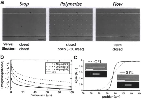
Pulsing frequency was fixed at 0.5 Hz. The compressed-air system exhibited a rapid reaction to th e d rivin g force... 2 7 Figure 1.9: Stop Flow Lithography (SFL) (a) Three steps in the SFL process. The first step is

stopping the flow ofpolymer solution. The second step is photopolymerization via flash of UV light through a mask. The final step is flowing out of microparticles using a pressure pulse. (b) Comparisons for particle throughputs of CFL and SFL. The throughput is a function ofparticle size. When particle size is getting smaller, the difference of throughputs is getting larger. (c) Comparisons for fluorescent signals of striped particles synthesized from CFL and SFL. Scale bars are 50 pm (a) and 100,pm (c). Figures adapted from ref 73. ... 28 Figure 1.10: A model for oxygen inhibited photo-polymerization (a) Schematic diagram of the

reaction -diffusion model. DIC images show measurements ofparticle width, x, and height, h. (b)

A plot for induction time ri as a function of Da. (c) A plot for the critical thickness of the

inhibition layer ie as a function of Da. Figures adapted from ref 75... 29 Figure 1.11: Barcoded hydrogel particles (a) A schematic depicting the synthesis process of barcoded

particles. The inserted fluorescent image show barcoded particles produced from the process. Figures adapted from ref 7. (b) The fluorescent image of color-coded particles. The colors were genera ted from ID photonic crystal structures of magnetic nanoparticles. Image adapted from

ref 76. (c) A fluorescent image of barcoded particles conjugated with fluorescently labeled viruses. Image adapted from ref 83. (d) High sensitivity of barcoded particles. The particles detected micro-RNAs at atomolar concentrations. Figures adapted from ref 78. Scale bars are 500 p m (b) an d pm ( )... 30 Figure 1.12: Bio-related applications of FL (a) Assembly of cell-laden hydrogel particles using a

railed microfluidic device. Image adapted from ref 84. (b) Biomimetic hydrogel particles. The particles were enough squishy to penetrate into a channel that had smaller dimensions than their sizes. Figures adapted from ref 86. (c) A fluorescent image of biodegradable particles. A

triangle particle was divided into two parts as the middle biodegradable part disappeared by erosion. Image adapted from ref 85. (d) Nanoem ulsion composite microgels. The nanoem ulsions allow for the release of drugs encapsulated in the gel particles, and reloading of drugs. Image adapted from ref 88. Scale bars are 10 pm (b) and 50 pm (c and d)... 31

(12)

Figure 1.13: Other applications of FL (a) A confocal image of a micro-gear for MEMs applications. The gear was fully compacted with glassy silica colloidal particles. Image adapted from ref 89.

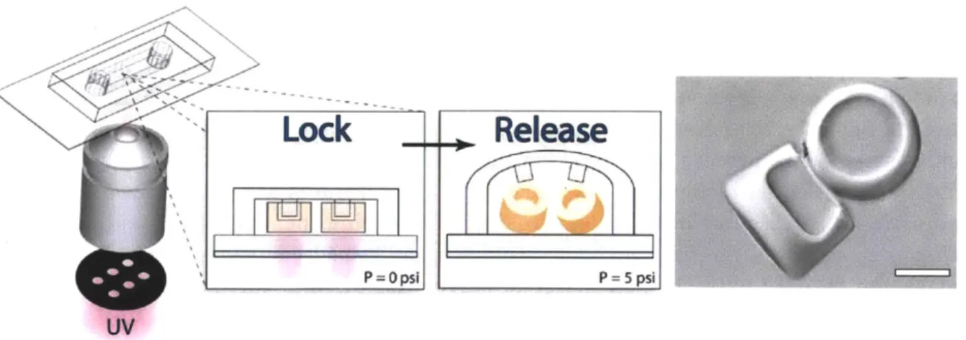
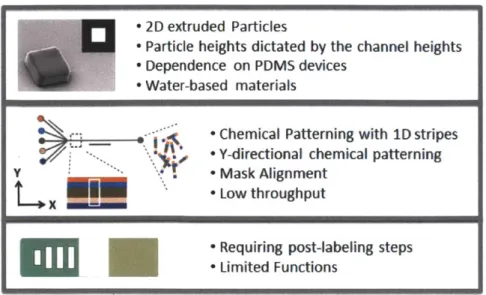
(b) Micro -actuators for MEMs applications. In the presence of external magnetic field, the actuator exhibited anisotropic motions because the structure had programmed magnetic anisotropy. Image adapted from ref 90. (c) Anisotropic amphiphilic particles. Particles with a large hydrophilic head (blue) and a small hydrophobic tail (red) were assembled at the interface of oil-in -water. Image adapted from ref 91. (d) Structural color printing. Magnetic nanoparticles were used to generate different structural colors by modulation of external magnetic fields. Image adapted from ref 92. Scale bars are 100,pm (a, b, and d), and 50pm (c) ... 32 Figure 1.14: Limitations in the primitive versions of flow lithography and barcoded particles. ... 33 Figure 2.1: Process of lock release lithography. First, structures are polymerized by shining bursts of

UVight through a transparency mask and a microscope objective. The structures, having a shape determined by the mask and channel topography, are 'locked" by relief structures in the channel topographies. Particles are "released" with channel deflection after a relatively high pressure (- 5psi) is applied to initiate flow. Differential interference contrast (DIC) image of

collection of 3D particles in the channel reservoir. ... 37 Figure 2.2: Measurements of membrane deflection at apex for membrane thickness [Ref 100]... 38 Figure 2.3: 3D particle synthesis from channels with negative topographies (a)-(d) Squares with

1-pm -high line-space patterns using 30-1-pm -high channel with negative line-space patterns on its floor and a square mask. (e)-(g) Squares with 10-pm -high gecko-type patterns using 20-pm -high channel with negative dot patterns on its ceiling and a square mask. (h)-() Table-like 3D

particles with 1-pm-high line space patterns on the top and 30-pm -high supports on the bottom using 30-pm -high channel with negative line-space patterns on both sides and a circle mask. Scale bars are (b) 100,pm (c, g, i) 50 pm, (d) 10 pm, and (f) 200 pm...40 Figure 2.4: Synthesis of variants by changing masks and/or channel topographies (a) Variants using

30-pm -high channels with same kinds of topographies of negative dots on their ceiling, but different cross mask. (b) Micro T-shirt with 3D MIT logo. Scale bars are (a) 200 pm and (b) 50 p m . ... 4 1 Figure 2.5: 3D particle synthesis from channels with positive topographies. Microcups with 30-pm

-deep voids were generated using 60-pm -high channel with positive dot patterns on its ceiling

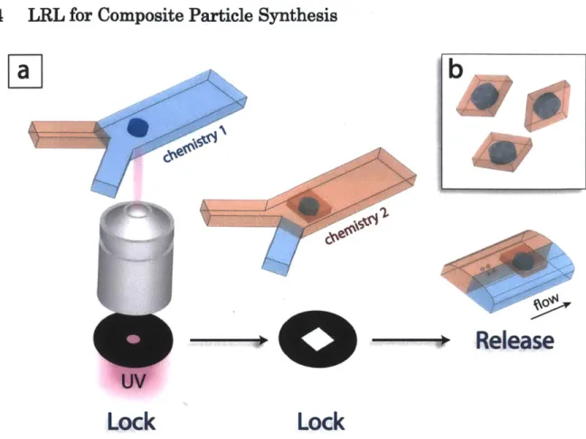
and a circle m ask. Scale bar is 50 pm . ... 41 Figure 2.6: Synthesis of composite particles. (a) A schematic diagram showing the synthesis of

composite particles. Locking structures with chemistry 1 are covalently linked to chemistry 2 through mask overlap and UV exposure after fluidic exchange with low pressure. Then, the composite structures are released by high pressure in both flows. (b) A schema tic description of particles produced by the process (a)... 42 Figure 2.7: Composite particles with two distinct chemistries. (a) DIC image of a composite particle

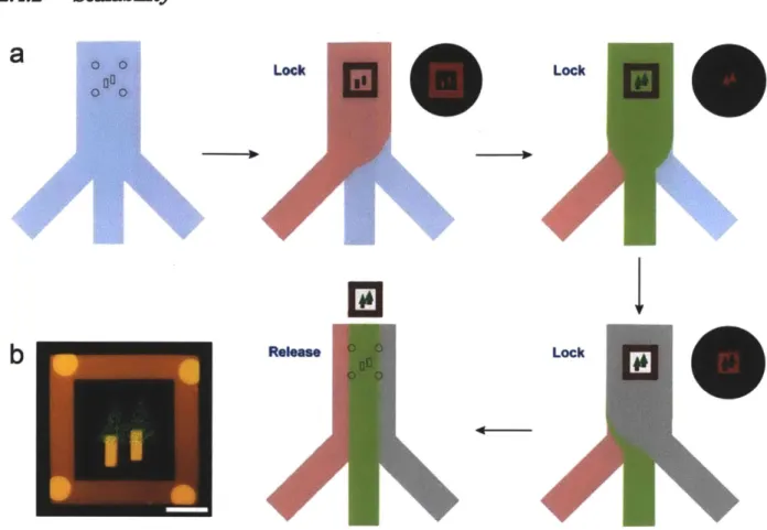
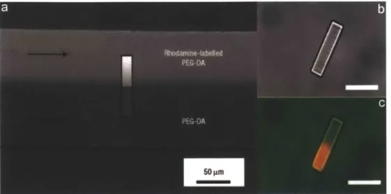
with a circular center and square exterior. (b) Fluorescence microscopy image of the particle shown in (a). (c) DICimage of a composite particle with interior features and border. (d) Fluorescence microscopy image of the particle shown in (d). Two streams containing PEG-DA and PEG-DA with rhodamine -labeled monomer were used to respectively present chemistry 1 and chemistry 2. Scale bars are 100 pm (a and b) and 50 pm (c and d)... 43 Figure 2.8: Composite particles with three distinct chemistries. (a) A schematic diagram showing the

synthesis of composite particles with three chemistries. First, we flow a prepolymer solution with red fluorophores, rhodamine-acrylate. Using a first mask, we generated a frame and two trunks of trees locked in the channel topographies. Then, in a low pressure, we replace the first prepolymer solution as a second one with 200 nanometer green fluorescent beads. Using a

(13)

second mask, we created leaves of trees. After that, we flow third prepolymer solution with no fluorophores in a low pressure. With a final mask, we connect trees with the frame. Finally, a high pressure flow is used to release the composite particle. (b) Fluorescence microscopy image of a composite particle synthesized in the process (a). Scale bar is 50 pm...44 Figure 2.9: Fluorescence microscopy images of multiple composite particles with different orientation.

(a) Composite particles with "fall trees" in a frame. (b) Composite particles with "spring trees" in a fram e. S cale bar is 100 pm ... 45 Figure 2.10: Functional particles. (a) Fluorescence and DIC images of "Venn diagram "particle

demonstrating interwoven (fluorescent monomer, orange) and excluded chemistries (beads, green) in polymerization overlap region. (b) Fluorescence and DIC images of a DNA detector particle with distinct probe regions. Shown are fluorescent images of a particle after incubation

with target #1 (green) or both targets #1 (green, insert in the top right corner). and #2 (red, insert in the top right corner). (c) - (e) Fluorescence images ofparticles with pH-responsive fins and a cross-shaped rigid support. The particle keeps its original 2D circle shape in low pH (c)

while in an alkaline pH, the fins bloom to form a 3D flower-like structure (d). (f) Fluorescence and DIC images of overlapping zig-zag-shaped particles with encapsulated entities. One strand contains 2 pm green fluorescent beads while the other has 5 nm red fluorescent strepta vidin protein. In all DIC images, particles have been outlined for clarity. Scale bars are 50 pm (a,b), an d 10 0 p m (c-f). ... 46 Figure 3.1: A schematic diagram for fabrication process of oxygen permeable two-layered PDMS

channels. A partially cured PDMS bottom channel is prepared on a glass slide via PDMS-PUA

-PDMS replica molding technique. Then, a top -PDMS channel is assembled on the bottom channel generating a two -layered gas permeable PDMS channel. ... 50 Figure 3.2: Hydrodynamic focusing lithography (HFL) for high -throughput synthesis of Janus

microparticles. (a) Schematic description for the creation of layered monomer flows. Pi and P2 represent the inlet pressures of top and bottom channel respectively. All inlet dimensions are 40 pm X 40 pm. Particles are synthesized after layered flows are widened up to 1 mm in a 40 pm

tall region of the channel. (b) A side view of flow focusing and particle polymerization. (c)A fluorescent image of 50 pm triangular particles with green (200 nm, green fluorescent beads)

and red (Rhodamine-A) layers. Hi and H2 are the heights of top (red) and bottom (green) layer in a particle. Scale bar is 50 pm. ... ... 51

Fi gure 3.3: Uniformity of Jan us particles synthesized at A, B, C, D and E spots across a 1 mm width channel. The intervals between spots are 100pm. Scale bar is 50pm. ... 52 Figure 3.4: Comparison ofmeasured H2H1 versus estimated flow ratio Q2/Qi. A simple

hydrodynamic resistance model predicts a curve for the relation. Scale bar is 20pm... 53 Figure 3.5: A schematic description of a PDMS channel used for creation of two layered flows... 54 Figure 3.6: Synthesis ofimulti-layered microparticles. (a) A schematic drawing for synthesis process

of tri-layered microparticles. In the stable layered flow, tri-phasic triangular particles can be synthesized using a mask with triangles. (b) Differential interference contrast (DIG)image of 50 pm tri -layered triangular particles (c) Magnified fluorescent image for the circled region of (b). Scale bars are 100jpm (b) and 50 pm (c). ... 57 Figure 3.7 Tri-layered microparticles with different aspect ratios (a) 20pm pentagonal particles

with aspect ratio 2. These particles contain rhodamine -acryla te in both top and bottom layers but no fluorophores in the middle layer. (b) 150 pm tri-layered ring particles with aspect ratio

0.4. Scale bars are 30 pm (a) and 100jpm (b)... 57 Figure 3.8: Synthesis of dual-axis layered microparticles. (a) A schematic diagram for synthesis

(14)

nm green fluorescent beads, 100 nm blue fluorescent beads and rhodamine-acrylates as

fluorophores. Inserted fluorescent images show dual-axis flows in a two-layered PDMS channel. (b) A fluorescent image to show a side view of a 40pm cross shaped particle with red, blue (in top) and green layers (in bottom) (c) A fluorescent image of mass -produced particles. Scale bars are 80 pm (b) and 10 pm (c). ... 58 Figure 3.9: Synthesis of four-layered sandwich microparticles. (a) A schematic diagram for synthesis process of four layered sandwich particles with dual layers in the middle. A -B is the intersection of the channel with dual-axis four layered flows. (b)-(d) Fluorescent images of a sandwich

particle generated by the process in (a). Scale bars are 50 pm. ... 59 Figure 3.10: Synthesis of five-layered sandwich microparticles. (a) A schematic diagram for synthesis

process of five layered sandwich particles with dual layers in the top and bottom. A -B is the intersection of the channel with dual-axis five layered flows. (b-c) DIC and fluorescent images of a sandwich particle generated by the process in (a). Scale bars are 50 pm... 59 Figure 3.11: Protein conjugation on particle sides. (a)A schematic diagram for preparation of

triangular particles with patterned protein coatings. The middle flow contains biotin -PEGA that is copolymerized in the particle. After incubation, the triangular particles are coated with streptavidin -cy3 on the sides. (b) A DIC image of the protein coated triangular particles. (c) A fluorescent image of (b). Scale bars are 50 pm. ... 60 Figure 4.1: NOA81 channel fabrication (A) Bottom layer of channel is created by sandwiching NOA

between glass substrate and SU-8 master mold bearing positive-relieffeatures and then curing with 10-min UVexposure. (B) Top layer is created in a similar fashion, using a different master mold and a silane-treated PDMS layer with inlet and outlet holes that align with the

corresponding SU-8 relief elements. Silane treatment of PDMS substrate facilitates bonding betw een PD M S and N OA ... 65 Figure 4.2: Inlet fabrication utilizing NOA81 capillary coating. (a) A schematic description of the

inlet fabrication process. (b) A SEM (Scanning Electron Microscope) image for intersection of an

NOA81 -coated PDMS inlet. During the sample cutting process, the hard NOA81 coating that originally covered the entire circumference of the inlet was broken, and the image provided shows only a portion of the original cylindrical coating. The white arrow indicates the remaining portion of the broken NOA81 coating. (c) A magnified SEMimage of (b). (d) An optical image to show the intersection of an evenly coated inlet. The NOA81 was coated with around 200 um thick on the PDMS substrate. All scale bars are 1 mm. ... 66

Figure 4.3: iCVD nano-adhesive bonding (a) Schematic description for the iCVD nano-adhesive bonding process. The nano-adhesive films ofpoly(4-aminostyrene) (PAS) and poly(glycidyl methacrylate) (PGMA) were deposited on top and bottom channel substrates, respectively, via iCVD. The two channel substrates are aligned and sealed together under vacuum via the ring-opening reaction of the newly generated amine and epoxy groups. (b) Color image of fully assembled channel mounted on a glass slide. The devices are optically transparent and can be used with photolithographic techniques. Scale bar is 1 mm. ... 67

Figure 4.4: Bonding NOA81 channels with various substrates. All scale bars are 1 cm... 68

Figure 4.5: iCVD nano-adhesive bonding (a) Schematic description for the iCVD nano-adhesive bonding process. The nano-adhesive films ofpoly(4-aminostyrene) (PAS) and poly(glycidyl methacrylate) (PGMA) were deposited on top and bottom channel substrates, respectively, via iCVD. The two channel substrates are aligned and sealed together under vacuum via the ring-opening reaction of the newly generated amine and epoxy groups. (b) Color image of fully assembled channel mounted on a glass slide. The devices are optically transparent and can be used with photolithographic techniques. Scale bar is 1 mm. ... 69

(15)

Figure 4.6: On -the-fly alteration ofparticle height with inert flows (a) Schematic of microparticle synthesis in gas-impermeable NOA channel. Particles were synthesized and then carried out of

the synthesis area using rapid, synchronized cycles of sh utter-media ted UV exposure and pressure -driven flow. (b) A schematic to describe the vertical flow focusing process. Instead of

volumetric flow rates, we con trolled pressures at the inputs to provide rapid alternation

between the flow and stoppage states. The middle monomer flow is sandwiched between top and bottom inert flows without mixing due to low Reynolds number flow conditions...70 Figure 4.7: A schematic description for two layered homogeneous NOA81 channels ... 72 Figure 4.8: On -the-fly alteration ofparticle height with inert flows (a) Schematic of microparticle

synthesis in gas-impermeable NOA channel. Particles were synthesized and then carried out of the synthesis area using rapid, synchronized cycles of sh utter-media ted UV exposure and pressure -driven flow. (b) A schematic to describe the vertical flow focusing process. Instead of

volumetric flow rates, we con trolled pressures at the inputs to provide rapid alternation

between the flow and stoppage states. The middle monomer flow is sandwiched between top and bottom inert flows without mixing due to low Reynolds number flow conditions...73 Figure 4.9: The inlet pressure relation to achieve symmetry condition (Qi =

Qs.

When we use a

typical pressure 3.0 Psi as P2, P3 and Pi have a linear relation with slopes and intercepts

depending on which m odel is applied... 75 Figure 4.10: Comparing modified hydrodynamic model with the previous model in achieving the

symmetry condition. (a)A schematic description for preparing tri-layered particles containing red dye in the middle layer. The dye was used to visualize symmetry of layers. (b) Optical images of synthesized particles using inlet pressures predicted by each model. The modified model gives more accurate prediction for inlet pressures to achieve the symmetry condition.... 76 Figure 4.11: A schematic diagram for flow profile in the channel ... 77

Figure 4.12: A plot for B versus Pi. B is the ratio of the volumetric flow rates of inert flow (Qi) divided by the volumetric flow rates of middle monomer flow (Q2). In this plot, P2 is fixed to 3.0

Psi while Psis the linear relation with Pi to satisfy the symmetry condition... 77

Figure 4.13: Particle height as a function of P1. Height of cylindrical particles was seen to vary with inlet pressures in a manner that matched predictions from the hydrodynamic resistance model. As shown in the graph, the Hm prediction compared well with measurements ofparticle heights.

... 7 8 Figure 4.14: On -the-fly alteration ofparticle heights in a PDMS device. (A)A schematic description

for the process adjusting particle heights with inert tuning fluids (B) An optical image of collected particles in a reservoir. (C) A SEMimage showing top and side ofparticles. (D)

Comparison with the heights of original particles that were synthesized with oxygen lubrication layers (-2 pm). The top particle has altered height of 19 pm while the bottom one has almost chann el h eigh t of 36 pm . ... 79

Figure 4.15: Transverse monomer diffusion (a) Experimental setup for measurement of diffusion coefficient of PEG-DA 575 in PEG 200 in a PDMS device. The green stream consists of PEG 200

90% (v/v), PI 5% (v/v), food coloring 4% (v/v), and rhodamine acrylate 10% (v/v), while the gray

stream is comprised of PEG-DA 575 94% (v/v), PI 5%1 (v/v), and rhodamine acrylate l1% (v/v).

"T"-shaped exposure mask was used to determine the penetration depth (3) of PEG-DA. (b) Fluorescence images ofparticles produced with various residence times. (c) Penetration depth as a function ofresidence tim e... 81 Figure 4.16: Variation of PEG-DA 575 bading percentage to determine critical gel point (~15%

monomer concentration) Synthesis was performed in PDMS devices, and all streams contained rhodamine acrylate for visualization ofparticle interfaces. ... 81

(16)

Figure 4.17: Schematic descriptions for time evolution of monomer concentration. We estimate theoretical maximum value of time, to, at which critical gel point front reaches walls of gas-impermeable device and induces particle sticking... 83 Figure 4.18: COMSOL simulation for time evolution of monomer concentration in a slit-like NOA81

device (a) Simulation solution indicates the maximum residence time is 5.1 s for the creation of particles at Hm= 20 pm. (b) A plot for monomer concentration versus z-distance. ... 85 Figure 4.19: Anisotropic particle synthesis from organic precursors (a) Triangular particle synthesis

with PEG 200 inert flows in an NOA channel from organic precursor containing PEG-DA 200, ruthenium dye (mixed with methanol (MeOH) and toluene), and PI (b and c) Brightfield and fluorescence images of triangular particles synthesized in (a). (d) Particle synthesis in NOA

device with water-insoluble monomers (trimethylolpropane triacrylate (TMPTA) and polyurethane acrylate (PUA), mixed with toluene) and P1 Inert flows consisted of Tergitol

surfactant to lower surface energy andprevent curvature in top and bottom faces ofparticle. (e and f) Images ofparticles synthesized from TMPTA and PUA. Scale bars are (b and c) 30 pm, (e) 100 p m , an d (f) 50 p m ... 86 Figure 4.20: Synthesis of near-infrared (NIR)-active anisotropic particles (a) NIR-active triangular

particle synthesis. NIR emitting CdTeSe/ZnS quantum dots (QDs) were physically entrapped in

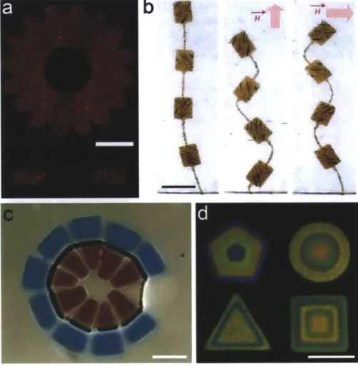
NOA polymer particles produced in NOA device. (b) Fluorescent signal intensity as a function of quantum dot loading concentration. Fluorescence was integrated over a circle ofradius 30 Pim centered on the triangular particles. Each point represents mean measurement from three particles; error bars represent standard deviation. ... 87 Figure 5.1: Production of magnetic barcoded particles. (a) Synthesis process of magnetic barcoded

particles. Stop flow lithography (SFL) is used to generate particles with three distinct chemical regions. The top stream is comprised of PEG-DA with food coloring and rhodamine A, while the

other streams consist of PEG-DA with probe oligonucleotide and magnetic beads, respectively. Downstream of the synthesis site, a PEG-DA perfusion stream is used to move un-incorporated magnetic beads into a waste outlet. (b) An experimental bright field image of the three phases flowing in the channel. The magnetic beads in the bottom flow are seen to be well-dispersed. (c) Dimensions of a magnetic barcoded particle. Coding holes are designed with the following

dimensions: '1' (12 x 15 pm), '2' (12 x 275 pm), and '3' (12 x 40 pm). The code in this

illustration is '2333' The scale bar is 50 ,um ... 93 Figure 5.2: Magnetic barcoded particles. (a)A bright field image (20x objective) of magnetic barcoded

particles with code '2333' (b) A fluorescent image of (a). (c) The side view of a magnetic barcoded particle in a bright field image (20x objective). (d) A fluorescent image of (c). (e) A bright field image (5x objective) of magnetic barcoded particles with code '0013' Scale bars are 50pm (a and

b), 25pm (c and d) and 100 pm (e). ... 94 Figure 5.3: AGMmagnetization curve for the commercial magnetic beads that were used in

synthesis of the magnetic barcoded particles. The saturation magnetization of the beads was found to be aroun d 28 em u/g... 95 Figure 5.4: AGM magnetization curve for magnetic regions (dried) of the barcoded particles. The

curve also shows superparamagnetic behavior, and no hysteresis was found... 96 Figure 5.5: Response of magnetic barcoded particles. (a) Response of magnetic barcoded particles to

out-of-plane (21.1-0. im T) magnetic field. (b) Response of magnetic barcoded particles to in

-plane (14. 7-0. im T) magnetic field. Scale bars are 100pm. ... 97 Figure 5.6: Orientation, transportation, and separation of magnetic barcoded particles. (a)

Reorientation of a magnetic barcoded particle in a microfluidic channel using a hand magnet. (b) Snapshots of magnetic transportation of a magnetic barcoded particle using a hand magnet.

(17)

The particle was transported towards a narrow region in the microfluidic channel used for single-particle scanning analysis. (c) Image of reoriented magnetic barcoded particles moving towards a hand magnet. (d) Bulk separation of magnetic barcoded particles using a hand magnet. Scale bars are 50pm (a and b), and 200 pm (c)... 98 Figure 5.7: Comparison between density-based separation strategy and magnetic force separation.

Fluorescent images of the magnetic barcoded particles after the ten rinsing steps of a DNA hybridization assay were carried out. Insert image clearly shows that magnetic force separation can provide a considerably smaller amount ofparticulate matter in the carrier solution than the density-based separation strategy. The scale bar is 50pm. ... 99

Figure 5.8: Incubation matrix. Particles with a fluorescent code region, an internal probe region, and a tail region were synthesized and incubated with either 0 or 200 amol of two different

biotinyla ted target oligonucleotides at 50 C for 90 min. Following incubation, probe-target complexes were labeled with strepta vidin -phycoerythrin (SAPE) at 21.5 C for 45 min. Particle

type 1 featured no probe, a magnetic tail, and code '2333'; type 2 featured probe 1, a magnetic tail, and code '2003'; type 3 featured probe 2, a magnetic tail, and code '0013'; type 4 featured probe 1, a non -magnetic tail, and code '2013.' Each plot shows the average of 5 scans of each particle type at the specified incubation condition. Horizontal axis is axial (length wise)position in pixels, and vertical axis is mean fluorescent intensity in arbitrary units. The mean signal across the width of the particle has been computed and plotted at each axial position. The red numbers above each scan indicate the mean fluorescent intensity measured in the probe region and in the tail region. The red bars in the first plot indicate the windows over which the

averages were taken. Quoted numbers represent the mean of five separate scans...100 Figure 5.9: Effect of Particle Density on Target Signal Each plot shows the average of 5 scans of

each particle type at the specified incubation condition. Data for (a) was taken from an

incubation of-50 particles of only type 4 with 200 amol of target 1. Data for (b) was taken from an incubation of -50 particles of each of the four types with 200 amol of target 2. For the two

cases, the total number ofparticles bearing probe complementary to the indicated target is roughly equal. The comparable signal intensities (63.2, 69.4 AU) in the probe regions indicate

that the lower signals seen for types 2 and 4 in Figure 5.8 are in fact the result of spreading the available target among a greater number ofparticles. Horizontal axis is axial (lengthwise) position in pixels, and vertical axis is mean fluorescent intensity in arbitrary units. Mean signals for each of the regions are calculated as described in Figure 5.8. ... 101 Figure 5.10: Porosity control for diffusion of target molecules The schema tic describes compositions

of a 4 layered particle produced by HFL. After incubating the particles with streptavidin, the proteins did not combine with the biotins in A2 region of the particles due to size exclusion. The scale ba r is 5 0 ,um . ... 103 Fi gure 5.11: Reinforced barcoded particles (a) Fluorescent image of soft PEG particles that were bent due to the mechanical instability. (b-c) Fluorescent images of-reinforced barcoded particles. The sandwiched particles consisted of three layers: (1) two soft porous layers in the top and bottom

of the particles (Red) and (2) a hard supporting layer in the middle of the particles (Green)... 103 Figure 5.12: Reinforced barcoded particles with 5 layered structures (a) A schematic description for

the structures of a 5 layered barcoded particle. The center consisted of a PEGDA 40% monomer while the top and bottom comprised of side-by-side stacked PEGDA 10% monomers. Each top and bottom layer has two regions of code and probe. (b) Fluorescent microscopy image of the

barcoded particles in (a). (c) Composite bright -field and fluorescent image of the barcoded p articles in (b)...10 4

(18)

Figure 5.13: Synthesis of Janus particles using structured microflows in a NOA 81 channel. (a) An optical image of a NOA81 device for Janus particle synthesis. In the first step, we prepared a two-layered NOA81 device with 5 inlets and 1 outlet. Using soft lithography, we could easily generate top and bottom NOA81 channels with geometries for the creation of 4

layered

flows. To

combine these two channels, we also used the iCVD nano-adhesive bonding method. (b) A schematic description for the generation of layered microflows which contain in their center side-by-side stacked monomers which are bounded on inert flows (c) A fluorescent image for Janus particles synthesized from this process. The scale bar is 50 pm... 105 Figure 5.14: Synthesis ofnear-infrared (NIR)-active barcoded particles (a) A schematic description

for NR-active multifunctional encoded particle synthesis. Using Tergitol for inert flows, Janus particles were created with a graphical barcode bearing near-infrared emitting QDs and a

separate probe region embedded with single-walled nanotubes (SWNTs) for label-free and real-time detection. (b) DIC and near-infrared photoluminescence images ofparticles from (a). The scale bar is 50 p m . ... 106 Figure 5.15: Synthesis of near-infrared (NIR)-active barcoded particles (a) Shift in emission

spectrum of embedded SWNTs upon introduction of 2.4 MHC. Blue arrow indicates most pronounced shift, produced by (8, 7)-type SWNT. (b) Intensity decay for (8,7)-type SWNT during H+ detection. Exponential quenching model was fit to the experimental data, providing

moderate proton quenching kinetic parameters...107 Figure 6.1: 3D folding of 2D patterned sheets (a) 3D structures self-assembled from magnetically

patterned sheets. Images adapted from ref 175. (b) 3D structures self-assembled from the interaction between elasticity and capillarity. Images adapted from ref 197 (c) 3D structures

self-assembled from 2D metal sheets with patterned mechanical properties. Images adapted from ref 198. Scale bars are 250pm (c)... 110 Figure 6.2: Designs of smart particles (a) A scheme illustrating three stages for folding of a magnetic

composite particle by magnetic fields. Image adapted from ref 175. b. A schematic illustrating shape -changing process of a magnetic composite particle with heat responsive polymer... 111 Figure 6.3: Oxygen permeable perfluoropolyether (PFPE) (a) A schematic depicting a simple

experiment to check the existence of oxygen lubrication layers. In the experiment, a droplet of PEGDA/PI was sandwiched between glass layers and polymerized by mask-defined UVlight. Photopolymerized PEGDA structures between glass slides were immobile even after 1000 seconds. (b) The same experiment was performed for PFPE layers. Photo -polymerized PEGDA

structures between the PFPE layers were mobile

just

after UV exposure. This validated that PFPE could provide oxygen lubrication layers. Scale bars are 100 pm... 112 Fi gure 6.4: SFL in a PFPE device (a) A schematic depicting the SFL process to synthesize triangular

particles in a PFPE device. By virtue of oxygen lubrication layers, PFPE devices can allow for the production of free-floating particles. (b) The inserted schematic shows a top view of the process (a). Bright-field and fluorescent images show particles synthesized in (a). (c) Synthesis of multifunctional barcoded particles. A mask with an array of barcode particle shapes was aligned on three phase laminar flows that were created in a PFPE device with multiple inlets. Bright-field and fluorescent images show the barcoded particles with three distinct

compartments. Scale bars are 100 pm (a) and 70pm (b)... 113 Figure 6.5: Comparison of SFL performance between PDMS and PFPE devices (a) Top view of

particles synthesized in both devices. The cylindrical particles were synthesized by SFL process using a mask with an array of 15 pm circles. For both devices, the diameters of sixteen particles were measured and plotted. The error bars indicate standard deviation. (b) Side view of

(19)

particles. The particles were toppled by stable laminar flow in microfluidic devices. Like (a), the particle heights were measured and plotted with error bars. ... 114 Figure 6.6: Comparison of solvent-based SFL between PDMS and PFPE devices (a) A schematic

depicting toluene -based SFL process in PDMS devices. The particles have curved shapes due to

the swelling of the PDMS walls. The precursor consists of water insoluble monomer

(polyurethane acrylate (PUA)), toluene, photoinitiator, and rhodamine acrylate. (b) Bright-field

and fluorescent miscopy images of curved particles. (c) The fluorescent signals of three particles

were quantitatively analyzed on particle distance using Image J software. (e) A schematic depicting toluene-based SFL process in PFPE devices. The particles have flat shapes due to

toluene resistance of PFPE devices. () Bright-field and fluorescent images of flat particles. (g) Like (c), the fluorescent signals of three particles were analyzed on particle distance...115 Figure 6.7: Droplet size modulation using the compressed-air flow control system. Images taken

downstream from a Tjunction demonstrate the size range that can be achieved by simple adjustment of the dispersed phase driving pressure. All scale bars are 50pm. ... 116 Figure 6.8: Synchronization of SFL in droplet-based microfluidics (a) A schematic depicting the

synchronization process. A droplet is stopped prior to SFL polymerization. Then, mask-defined particles are generated inside the droplet. After that, the droplet containing anisotropic particles is released by flows. (b) A fluorescent image ofparticles prepared by process (a). Each

droplet contains a triangle particle inside. (c) Sequential DIC images to show the experimental process. Scale bars are 50 pm . ... 117 Figure 6.9: Advanced barcoded particles for living cell assays (a) A schematic depicting the synthesis of extracellular matrix (ECM) microbeads encapsulating anisotropic particles. (b) A schematic showing the final product in process (a). (c) Living cell assays. During cell cultures on ECM microbeads, interior barcoded particles can be used to detect biomolecules secreted from living

(20)

List of Tables

Table 3.1 Geometries of a PDMS channel used for creation of two layeredflows ... 55

Table 3.2 Estim ated pressures and Q2/Qi... 56

Table 4.1 Summary for the maximum particle synthesis throughput for each type of FL ... 71

Table 4.2 Geometries of a two layered homogeneous NOA81 channel... 72

Table 4.3 Estimation of hydrodynamic resistances, R1 and R5... 74

Table 4.4 Estimation of hydrodynamic resistances, R3...74

Table 4.5 Estimation of hydrodynamic resistances, R2... .. . . . .. . . .. . . . .. . . . .. . . .. . . 74

Table 4.6 Comparison of hydrodynamic resistances estimated from two suggested models ... 74

Table 4.7 Estimated diffusivity of PEGDA 575 in PEG 200... 82

Table 5.1 Design of the four different magnetic barcoded particle types. ... 99

(21)

Chapter 1 In troduction

Recently, flow lithography (FL) has emerged as a promising way to prepare complex anisotropic particles, combining photolithography with microfluidic-based methods. This thesis is focused on the developments of advanced flow lithography to achieve much higher degree of geometrical and chemical complexity of particles than the primitive versions of FL. Also, advanced barcoded particles are proposed as a demonstrative application of the new techniques.

1.1 Anisotropic Multifunctional Particles

Anisotropic multifunctional particles hold great potentials in drug delivery [1-3], tissue engineering [4-6], sorting media [7-9], smart materials [10-15], optics [16], microelectromechanical systems [17-19], and building blocks [20-22] for self-assembled, dynamic structures with complex functionality. One of the simplest multifunctional particles is spherical Janus particles. As inferred from Janus, the name which means two-faced Roman god, the particles have two compartments of distinct chemical or physical properties. Although the form is simple, the spherical Janus particles have yielded entirely different applications that homogeneous microspheres cannot reach to. A simple example is Janus microspheres that have hydrophobic and hydrophilic surfaces. Once these particles can be spread out on the water, the hydrophilic regions are dipped into water leading to face-up of hydrophobic areas. Then, the hydrophobic coated area can provide so-called 'lotus effect' of antifogging and self-cleaning, and be used for the preparation of superhydrophobic

(22)

films on car or building windows [23]. Another example is dichromatic Janus microspheres.

These particles can be electrically or magnetically controlled for face-up direction, and used

as pixels of flexible bead displays or papers [24, 25]. Janus microspheres were also of

interest in assembly as anisotropic building blocks [26-30]. Furthermore, the particles can

be used for optical probes [31] and self-propulsion [32, 33].

b

0

_*

_e*

.

Ha0.50*

Figure 1.1: Applications of spherical Janus particles (a) Water-repellent Janus microspheres. The particles were used to form a super-hydrophobic monolayer on water. Then, a water droplet was sitting on the layer. The Image was adapted from ref 23. (b) Bicolored Janus microspheres. By varying the direction of an external magnetic field, the orientations of Janus particles were changed switching fluorescent signals. The particles can be used for magnetoresponsive bead display. Images adapted from ref 25. (c) Magnetic Janus microspheres. The particles were self-assembled in Zig-Zag structures in response to in -plain magnetic fields. Images adapted from ref 30. (d) Self-propelling Janus microspheres. The particles get propulsion force from uneven degradation rates of hydrogen peroxide. The image was adapted from ref 31. Scale bars are 1 cm (a), 25 pm (c, left) and 100 pm (c, right).

When physical or chemical structures of particles are getting complex, other interesting

applications can emerge. Gracius and co-workers have used geometrically and chemically

patterned particles to create 3D electronic circuits that had not been achieved with any

other methods [34]. Using particle self-folding, his group also developed micro-grippers to

capture targets [11, 35, 36] or micro-containers to load cells [37, 38]. The entities-loaded

particles were further traveled to the final destination by the remotely controlled

electromagnetic field [11, 36, 37]. When such complex particles hold even biocompatibility,

(23)

they can be used for new applications for the biomedical areas such as diagnostics, therapeutics and imaging. One example can be anisotropic building blocks which are patterned with different cell lines for tissue engineering [39-41].

Figure 1.2: Applications of anisotropic multifunctional particles (a) 3D electronic circuits. The structure was created from the assembly of truncated octahedron particles. The Image was adapted from ref 34. (b) Micro-grippers. The particles can catch and release target entities by chemically or thermally triggered actuation. The right fluorescent image shows that a micro-gripper locomote gripping samples. Images adapted from ref 11 and 35. (c) Bottom-up assembly of cell-laden anisotropic particles. The building blocks were assembled into the multi-component constructs by hydrophobic interaction. Images adapted from ref 39. Scale bars are 100 pm (c, left 4 images) and 200pm (c, right).

1.2 Current Methodologies

The enormous potentials of anisotropic multifunctional particles have inspired scientists to develop various fabrication methods. Complex 3D particles can be synthesized using multi-photon fabrication [42-46]. With 100 nm feature resolution, the technique has provided precise control over particle geometry in all dimensions. Unfortunately, the synthetic way has not been widely used for mass-production of 3D particles as the technique is prohibitively time consuming. To partially overcome this, it has been used to generate masters for soft-molding [45].

(24)

a

Figure 1.3: 3D particle synthesis (a) A schematic depicting experimental setups for two-photon lithography. Figure adapted from ref 44. (b) Venus Statue. The micro-statue was fabricated using the setup in (a). Image adapted from ref 44. (c) Inter-locking chain. The micro-chain was fabricated from multi-photon absorption fabrication. Images adapted from ref 43. Scale bar is 100pm (c).

Anisotropic particles could be also introduced by off-wafer fabrication [47-49]. The advantage of this process is the high-throughput synthesis of particles at a rate of 108 particles/min. However, the use of photoresist materials renders this approach suboptimal for many biological applications. In addition, the layer by layer process makes the chemical patterning limited to layered motifs. Alternatively, template-assisted particle fabrication [50-52] could be used to create geometrically complex particles with sub-micrometer dimensions. Unfortunately, this method is largely ineffective at producing particles with chemical anisotropy or patterning, as the precursor liquid is simply isolated in a non-wetting template and then crosslinked in situ. Although one-dimensional striped particles have been generated [53], the synthesis requires complex steps including multiple evaporation-refilling-crosslinking procedures, and the process cannot be applied to non-volatile precursors.

a

"b

Figure 1.4: Mass-production of anisotropic particles (a) Off-wafer synthesis. The schematic describes the fabrication process. Inserted images show micro-alphabets and layered composite particles. Figures adapted from ref 48 and 49. (b) PRINT fabrication. The schematic describes the PRINT process. Inserted image shows micro-cubes. Figures adapted from ref 51 and 52. Scale bars are 3 pm.

Other liquid-phase particle synthesis methods have had limited success in creating geometrically and chemically anisotropic particles due to the tendency of liquid systems to

(25)

adopt arrangements that minimize surface energy. In current liquid-based methods such as batch nucleation [54], emulsification [55], microreactor production [56, 57], droplet-based microfluidics [24, 58-61], droplet template fabrication [62, 63], co-jetting [64], and microcutting [65], the particle geometries have been restricted to spheres, deformed spheres, or cylinders.

b

* Unsele

* ultrasound reaction

--- 10nm Pbase II

Figure 1.5: Other liquid-phase synthesis methods (a) SEM and TEM images of nanoparticles synthesized from batch nucleation. Images adapted from ref 54. (b) A schematic depicting the emulsification process. Figure adapted from ref 55. (c) Droplet-based microfluidics. Images adapted from ref 24. (d) An optical image for a micro-doughnut particle prepared by the droplet-template fabrication method. Image adapted from ref 63. (e) Electrojettting fabrication for the synthesis of Janus nanoparticles. Figure adapted from ref 64. (f) Micro-cylinders prepared by micro-cutting fabrication route. Images adapted from ref 65. Scale bar is 500,pm (d).

1.3 Flow Lithography

Microfluidic methods provide a flexible toolset for patterning precursor liquids in the synthesis process. The low Reynolds number regime of microfluidic devices offers several advantages that can be exploited for the generation of nano- and microparticles [66, 67]. Complex laminar flow patterns can easily be established in microfluidic channels without the need for physical separators, enabling a range of applications that cannot be achieved with more traditional liquid handling technologies [68-71]. Flow lithography (FL) is a versatile technique that combines photolithography with the capabilities of microfluidic methods for the high-fidelity synthesis of anisotropic gel microparticles [72, 73]. In this technique, photomask-defined shapes can be rapidly printed onto monomer flows, providing precise control over particle size, geometry, and chemical patchiness.

50 pm

(26)

1.3.1 Continuous Flow Lithography (CFL)

In CFL, the first form of flow lithography, mask defined shapes are patterned into a continuously flowing photo-polymerizable monomer stream [72]. The technique can fabricate virtually any two-dimensional particle by simple mask exchanges. The nexus of this technique is the lubrication layer (-lum thick) which is induced by atmospheric oxygen diffusing in through the porous PDMS and locally inhibiting polymerization. By virtue of this layer, particles formed via photo-polymerization are advected through unpolymerized prepolymer liquids without sticking to the PDMS walls.

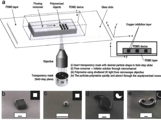
a

Rowing

PDMS layer monomer PDMS device Glass slide

z inhbion layer

Transprency mask (bid-stop A )

\ PDMS layer

P

) Insert tnsparency mask with desired partcle shapein eld-Sop sider (i) Flow mononw + initiator solution1hrough microchannel

h

W polymmusing shuttered LN ihtfrom microscope objecive

(n) The pericles polymerize qucidy and advect through the unpolymerized monomer

Figure 1.6: Continuous Flow Lithography (CFL) (a) A schematic diagram of CFL process. (b) - (e) Differential Interference Contrast (DIC) images of various microparticles prepared by CFL. Scale bars are 10 um. Figures adapted from ref 72.

In co-flowing laminar streams, CFL can be also used to generate multifunctional particles. Figure 1.7a shows the schematic diagram for synthesis of Janus particles. The widths of the streams in Figure1.7a can be altered by changing the flow rates of the streams, controlling

(27)

over both functional areas. However, particles with arbitrary chemical patterns cannot be achieved by CFL because the chemical patterning relies on stream lines (Fig. 1.7c).

Figure 1.7: Synthesis of Janus particles (a) A schematic diagram showing the CFL process for the synthesis of Janus particles. (b) - (c) DIC and fluorescent images of a Janus particle synthesized in

the process (a). Scale bars are 100pm. Figures adapted from ref 72.

1.3.2 Stop Flow Lithography (SM)

a

3-WaySolenoid

b

Compressed or In-house tor Itor DU

- Compressed-air Flow Control System Ideal

400-I 11

1 2

t (s)

Figure 1.8: Compressed-air flow control system (a) Schematic of the pressure manifold and its attachment to a two-inlet microfluidic device. Compressed air is down regulated and then passed

through a three -way solenoid valve that serves to either pressurize the manifold (open) or vent to the atmosphere (closed). Two control channels, each with its own sample arm and relief needle valve, are pictured branching off the main supply line. (b) Pulsed-flow operation. Pulsing frequency was fixed

at 0.5 Hz. The compressed-air system exhibited a rapid reaction to the driving force. SClose C . lam -Regula Needle Valve 0

Advanced flow lithography and barcoded particles

KI

WAN BONG

ARCHIVES

Advanced Flow Lithography and Barcoded Particles

Ki Wan Bong

Acknowledgments

Table of Contents

List of Figures

Qs.

layered

just

List of Tables

Chapter 1

In troduction

1.1

Anisotropic Multifunctional Particles

films on car or building windows [23]. Another example is dichromatic Janus microspheres.

These particles can be electrically or magnetically controlled for face-up direction, and used

as pixels of flexible bead displays or papers [24, 25]. Janus microspheres were also of

interest in assembly as anisotropic building blocks [26-30]. Furthermore, the particles can

be used for optical probes [31] and self-propulsion [32, 33].

b

*

e*

.

When physical or chemical structures of particles are getting complex, other interesting

applications can emerge. Gracius and co-workers have used geometrically and chemically

patterned particles to create 3D electronic circuits that had not been achieved with any

other methods [34]. Using particle self-folding, his group also developed micro-grippers to

capture targets [11, 35, 36] or micro-containers to load cells [37, 38]. The entities-loaded

particles were further traveled to the final destination by the remotely controlled

electromagnetic field [11, 36, 37]. When such complex particles hold even biocompatibility,

1.2

Current Methodologies

a

a

"b

b

1.3

Flow Lithography

1.3.1

Continuous Flow Lithography (CFL)

a

P

h

1.3.2

Stop Flow Lithography (SM)

a

b

_*

_e*