Constraining hydrological model parameters using water isotopic
compositions in a glacierized basin, Central Asia
Zhihua He
a,1,⁎, Katy Unger-Shayesteh
a,2, Sergiy Vorogushyn
a, Stephan M. Weise
c,
Olga Kalashnikova
d, Abror Gafurov
a, Doris Duethmann
e, Martina Barandun
f, Bruno Merz
a,baGFZ German Research Centre for Geosciences, Section Hydrology, Telegrafenberg, Potsdam, Germany
bUniversity of Potsdam, Institute of Earth and Environmental Science, Potsdam, Germany
cUFZ Helmholtz Centre for Environmental Research UFZ, Department Catchment Hydrology, Halle, Germany
dCAIAG Central Asian Institute of Applied Geosciences, Department Climate, Water and Natural Resources, Bishkek, Kyrgyzstan
eInstitute of Hydraulic Engineering and Water Resources Management, Vienna University of Technology (TU Wien), Vienna, Austria
fDepartment of Geosciences, University of Fribourg, Fribourg, Switzerland
A R T I C L E I N F O
Keywords: Water stable isotope
Isotope-hydrological integrated modeling Quantification of runoff components Glacierized basins
A B S T R A C T
Water stable isotope signatures can provide valuable insights into the catchment internal runoff processes. However, the ability of the water isotope data to constrain the internal apportionments of runoff components in hydrological models for glacierized basins is not well understood. This study developed an approach to si-multaneously model the water stable isotopic compositions and runoff processes in a glacierized basin in Central Asia. The fractionation and mixing processes of water stable isotopes in and from the various water sources were integrated into a glacio-hydrological model. The model parameters were calibrated on discharge, snow cover and glacier mass balance data, and additionally isotopic composition of streamflow. We investigated the value of water isotopic compositions for the calibration of model parameters, in comparison to calibration methods without using such measurements. Results indicate that: (1) The proposed isotope-hydrological integrated modeling approach was able to reproduce the isotopic composition of streamflow, and improved the model performance in the evaluation period; (2) Involving water isotopic composition for model calibration reduced the model parameter uncertainty, and helped to reduce the uncertainty in the quantification of runoff compo-nents; (3) The isotope-hydrological integrated modeling approach quantified the contributions of runoff com-ponents comparably to a three-component tracer-based end-member mixing analysis method for summer peak flows, and required less water tracer data. Our findings demonstrate the value of water isotopic compositions to improve the quantification of runoff components using hydrological models in glacierized basins.
1. Introduction
Glacierized basins substantially provide freshwater for the down-stream agriculture and potable water supply, especially in warm and dry years (Prasch et al., 2013). However, changes in climate are altering the short- and long-term characteristics of runoff processes in these basins (Stahl and Moore, 2006; Stahl et al., 2008; Duethmann et al., 2015). Understanding changes in runoff generation processes is
there-fore critical to the downstream water resource utilization, considering the particular vulnerability of snow and glacier-dominated environ-ments to changing climatic conditions (Barnett et al., 2005; Penna et al., 2014). Sound quantification of glacier melt, snowmelt, rainfall and groundwater contributions to the streamflow helps to understand
the changes in freshwater availability provided by glacierized head-water basins (Jost et al., 2012).
Hydrological modeling is an effective tool to quantify changes in individual runoff components, providing insights into the catchment dynamics. A number of studies have modeled the contributions of runoff components to streamflow in glacierized basins (Jost et al., 2012; Lutz et al., 2014; He et al., 2015). For example,Verbunt et al. (2003)
investigated the contributions of snowmelt and glacier melt to total runoff using a spatial-gridded hydrological model in high alpine catchments in Switzerland.Engelhardt et al. (2014)analyzed the spatial variations and temporal evolution of the water sources, including snowmelt, glacier melt and rainfall, by means of a distributed hydro-logical model in a Norway glacierized basin. Zhao et al. (2013)
⁎Corresponding author.
1Now at Centre for Hydrology, University of Saskatchewan, Saskatoon, Saskatchewan, Canada. 2Now at German Aerospace Center (DLR), International Relations, Linder Höhe, Cologne, Germany.
http://doc.rero.ch
estimated the contribution of glacier melt to runoff using hydrological modeling for a glacierized catchment in Central Asia. However, the large calibration uncertainty in hydrological model parameters could lead to incorrect estimation of the runoff component shares (Nolin et al., 2010; Finger et al., 2015). In glacierized basins, the hydrological model typically integrates complex runoff generation processes. In ad-dition, uncertainties in the forcing data for the hydrological models are high due to the commonly sparse climatic gauge network (Immerzeel et al., 2014; Tarasova et al., 2016). Both effects can lead to considerable compensation between different runoff components in the hydrological model. A hydrological model could produce rather similar performance on the simulation of the total runoff by overestimating (under-estimating) one runoff component to compensate the underestimation (overestimation) of the other runoff component. For example, a hy-drological model could overestimate (underestimate) the glacier melt runoff and underestimate (overestimate) the precipitation-triggered runoff (i.e., sum of rainfall and snowmelt) to produce high performance for the simulation of total runoff, due to the insufficient accuracy in model inputs (Duethmann et al., 2013; Duethmann et al., 2014; He et al., 2014; Immerzeel et al., 2015). Therefore, multi-criteria calibra-tion methods using coupled hydrological observacalibra-tions, including gla-cier mass balance, satellite remotely-sensed snow cover area and ob-served discharge, were adopted to reduce the model uncertainty (Koboltschnig et al., 2008; Parajka and Blöschl, 2008; Konz and Seibert, 2010; Schaefli and Huss, 2011; Duethmann et al., 2014; Duethmann et al., 2015; Finger et al., 2015).
However, there is still significant uncertainty in the quantification of runoff components even when calibrating the hydrological model using both discharge and glacier/snow cover observations (Duethmann et al., 2015). Water stable isotopic compositions provide insights into the dominance of various runoff processes on total runoff, bearing the potential to further constrain the internal apportionments of runoff components (Soulsby and Tetzlaff, 2008; van Huijgevoort et al., 2016). Recently, water stable isotope data have been increasingly in-tegrated into hydrological models to improve the understanding of dynamics in runoff processes. Ala-aho et al. (2017a) simultaneously simulated theflux, storage and mixing of water and water isotopes in three snow-influenced catchments. Some other studies in non-glacier-ized basins used water isotopes to reduce the model calibration un-certainty, attempting to achieve the‘right answers for the right reasons’ (Seibert et al., 2003; Weiler et al., 2003; Stadnyk et al., 2005; Dunn and Bacon, 2008; Stadnyk et al., 2013). For instance,Birkel et al. (2010)
highlighted that isotope-tracer data helped to constrain the acceptable behavioral parameter sets and reduce model’s degrees of freedom.
Capell et al. (2012) found that using isotope-tracer data reduced parameter uncertainties and helped improving the model structure for reproducing spatial variabilities of runoff processes. Tetzlaff et al. (2015)demonstrated that integrating water isotopes into hydrological models could help to test the conceptualizations of physical processes in the model. However, the value of the water stable isotope measure-ments for model calibration in glacierized basins has not been in-vestigated in previous studies. As far as we know, water isotopic com-positions have not yet been integrated into glacio-hydrological models, partly due to the logistical challenges related to long-termfieldwork and water sampling in cold and high-altitude environments. Therefore, the extent to which the water isotope data can constrain the internal apportionments of runoff components in hydrological models for gla-cierized basins is not clear.
The tracer-based end-member mixing analysis approach is another widely used method for the quantification of runoff components in glacierized basins (Dahlke et al., 2014; Engel et al., 2016). For instance,
Pu et al. (2017)estimated the contribution of glacier and snow melt-water to streamflow in a glacierized basin in the southeast margin of the Tibetan Plateau using the signatures ofδ18O andδ2H. Maurya et al. (2011)employed a three-component end-member mixing method to estimate the fraction of glacier melt runoff in a Himalayan river using
δ18
O and electrical conductivity. However, uncertainties in the con-tributions of runoff components estimated by the tracer-based end-member mixing method are typically large, partly due to the strong spatial and temporal variability in the water tracers (Joerin et al., 2002). Difficulties in field sampling and seasonal inaccessibility of
water samples in glacierized basins enhance the uncertainty in the quantification of runoff components (Rahman et al., 2015).
Against this background, we integrated the water isotopic compo-sitions of runoff components into the WASA hydrological model (model of Water Availability in Semi-Arid environments,Güntner and Bronstert 2004) and developed an isotope-hydrological integrated modeling ap-proach in a glacierized basin in Central Asia. The objective of this study is to investigate the value of the water stable isotope data for model calibration, as well as the ability of the proposed modeling approach for constraining the internal apportionments of runoff components for a glacierized basin. To achieve this goal, we compared an isotope-aided calibration approach with a common multi-criteria calibration ap-proach which used discharge, remotely-sensed snow cover area and glacier mass balance data in the study basin. Specific questions ad-dressed are two-fold: (1) What benefits can be gained for model cali-bration by incorporating the simulation of water isotopic composition into hydrological model in glacierized basins? (2) Is the isotope-hy-drological integrated modeling approach superior to a three-component tracer-based end-member mixing analysis method (abbreviated as tracer-based mixing method hereinafter) for the quantification of runoff components in summer peakflow periods?
The paper is organized as follows: A brief description of the study area and data collection is provided inSection 2. InSection 3, we de-scribe the proposed isotope-hydrological integrated modeling ap-proach, as well as the model calibration methods.Section 4presents the performance of the isotope-hydrological model, parameter un-certainties, and the contributions of runoff components. We discuss our results in relation to the literature and the limitations of this study in
Section 5, followed by conclusions inSection 6.
2. Study area and data collection 2.1. Study area
The Ala-Archa basin is located in Kyrgyzstan, Central Asia, at the northern edge of the Tien Shan mountain system (74°24′ E–74°34′ E; 42°25′ N–42°39′ N,Fig. 1). It has an area of 233 km2, approximately
17% of which is glacierized. The basin spreads throughout an elevation range from 1560 to 4864 m above sea level (a.s.l.). Approximately 83% of the Ala-Archa glacierized area consists of large valley glaciers, with about 76% of the total glacierized area located between 3700 and 4100 m a.s.l. (Aizen et al., 2007). The annual mean vegetation coverage is around 28% in this basin. Snowmelt runoff feeds the river streamflow during the melt period from March to September. Glacier melt runoff mainly feeds the river streamflow from July to September. The largest daily discharge generally occurs in July-August with a magnitude of around 25–40 m3/s, while the lowest daily discharge in
January-Feb-ruary is only around 1.9 m3/s. The long-term annual mean precipitation and temperature are 560 mm and 2.6 °C, respectively, based on the data series recorded at the Alplager station at 2100 m a.s.l. for the period 1970–2000. Precipitation mainly occurs in the form of snowfall in winter and has peak storms in the spring-summer months (Aizen et al., 1995, 2000, 2007). Water availability in the Ala-Archa River is critical for the downstream irrigated agriculture and the potable water supply. 2.2. Hydrometeorological and cryosphere data
Since the 1970 s, daily precipitation, air temperature, humidity and global radiation have been recorded at the Baitik (1580 m a.s.l.) and Alplager (2100 m a.s.l.) meteorological stations run by Kyrgyz Hydromet Service (Fig. 1). The recorded relative humidity in air at the
Baitik and Alplager station are generally larger than 50% in both summer and cold seasons. Mean daily streamflow has been measured at the Ala-Archa hydrologic station (close to the Baitik meteorological station) at the basin outlet since the 1960s.
The annual glacier mass balance (GMB) of the Golubin glacier (red polygon inFig. 1, ranging from 3320 to 4350 m a.s.l.) has been mea-sured during 1973–1993 and 2011-present (Hoelzle et al., 2017). The glaciological ablation and accumulation measurements were dis-tributed over the entire glacier surface and repeated annually. The point measurements were extrapolated to the glacier surface using a model-based inverse distance algorithm (e.g. Huss et al., 2009; Barandun et al., 2015) and the area weighted mean provides the annual glacier-wide mass balance. Additionally, the mass balance was calcu-lated for every 100 m elevation band and used to calculate the mass balance gradient with elevation (Hoelzle et al. 2017). Here, we used specific mass balance calculated for each elevation band for hydro-logical model calibration. The data was collected, analyzed and re-ported to the World Glacier Monitoring Service (WGMS) under the standard protocol (Hoelzle et al., 2017).
The Moderate Resolution Imaging Spectroradiometer (MODIS) daily snow cover products (MOD10A1 and MYD10A1) with a spatial re-solution of 500 m processed by the cloud removal procedure MODSNOW-Tool (Gafurov et al., 2016), were also explored for model calibration.
2.3. Isotope data
Weekly streamflow samples have been directly collected from the river channel near the Baitik (Ala-Archa hydrologic station) and Alplager meteorological stations since July 2013. The streamflow grab
samples were collected by station operators from the river around noon (but maybe not exactly at the same time) every Wednesday. Precipitation samples have been collected at the Baitik and Alplager meteorological stations since January 2013. The precipitation events were collected from plastic rain collectors at the meteorological stations and accumulated over one month in a rain container, from where a mixed sample was collected for monthly isotopic analysis. To act against the effect of evaporation, the rain container for monthly pre-cipitation accumulation wasfilled by a thin mineral oil layer before the collection of precipitation and stored in a shade room. Precipitation volumes were collected as immediately as possible after the rainfall/ snowfall event.
Glacier melt grab samples were collected annually during the summer field campaigns. Flowing meltwater on the Golubin glacier surface at various elevation bands in the ablation zone were collected to consider the spatial variability (i.e., points G1-4 inFig. 1, with elevation ranging from 3280 m to 3520 m).
Snowmelt and groundwater grab samples were occasionally col-lected during the warm season (March to October), due to the heavy snow coverage and limited catchment accessibility in the cold season. At each sampling site (points S1-3 inFig. 1), snow samples were col-lected by using a pure polyethylene plastic tube. We drilled the pure plastic tube into the snowpack to collect the whole snow layer. All the snow collected by the tube was poured into a plastic bag and stored in a cooling box. Snowmelt samples were then collected from the meltwater inside the bag when all the snow had melted out. The depth of the sampled snow layers differed at the sampling sites, ranging from 10 cm to 150 cm. Groundwater samples were collected from one spring draining to the river at the foot of a hillslope at point W1 (Fig. 1).
All samples were collected in pure polyethylene plastic bottles and
Fig. 1. Study area and water sampling points.
stored at 4 °C before the analysis in the Helmholtz Center for Environmental Research (UFZ) laboratory (Department of catchment hydrology, Halle in Germany). Isotopic compositions were analyzed with Laser-based infrared spectrometry (LGR TIWA 45, Picarro L1102-i) and calibrated against the common VSMOW scale with a precision of δ18O: ± 0.25‰ and δ2H: ± 0.4‰, respectively. Electrical Conductivity
(EC) in the water samples was measured in situ or in laboratory using portable EC/PH/TDS meters. Strict quality control procedures have been implemented for the isotope and EC data, discarding abnormal values caused by evaporation effects and sampling errors (for example, samples that experienced significant evaporation before the lab isotope analysis, and abnormal EC values caused by sediments from the sam-pling sites and significant laboratory measurement error were dis-carded).
The measured tracer characteristics of various water sources are summarized inTable 1. Theδ18O of precipitation generally shows the
largest variability with a coefficient of variation (CV) of 0.53 at the Baitik station, followed by the snowmeltδ18O which exhibits a CV of
0.26. As expected, the glacier melt and snowmelt show the most de-pletedδ18O among the water sources. The groundwater shows only minor variability in theδ18O as can be expected. Snow and glacier melt
present the lowest EC value, while groundwater shows the highest EC. The seasonality of EC characteristics of various water sources is pre-sented inFig. 2. The EC of streamflow reached its highest value in
winter, and showed low value in summer. 3. Methodology
3.1. Isotope-hydrological integrated modeling approach
The semi-distributed hydrological model WASA (Model of Water Availability in Semi-Arid Environments) originally developed by
Güntner and Bronstert (2004)was adopted in this study. It has been extended for snow and glacier melt processes and successfully applied in Central Asian mountain basins (Duethmann et al., 2013; Duethmann et al. 2015). The WASA model is based on the discretization of the landscape into model units according to soil properties, land cover and elevations. To set up the WASA model, the whole Ala-Archa basin was divided into 404 units, with an average size of around 0.58 km2(about
twice of the size of a MODIS pixel). Snowmelt and glacier melt on model units were calculated using a temperature-index approach (Hock, 2003), with two different degree-day factors for snow and gla-cier (Table 2). To differentiate between rainfall and snowfall, a
threshold temperature (Tm, set as 2.23 °C fromHe et al. 2018) was used.
The threshold temperature for melting (To) in the degree-day module
was set to the same value as Tm. Annual GMB was calculated for the
hydrological years from September to August by subtracting snowmelt and glacier melt from snowfall on the glacierized areas, in order to compare it with the GMB measured in the field typically in late summer. TheΔh-approach (parameterization for the changes in glacier thickness) was implemented in the WASA model to account for mass balance redistribution with glacier elevation range and account for glacier thickness and area changes (Huss et al., 2010). More details on the model structure can be found inHe et al. (2018). Monthly lapse rates of precipitation and temperature were derived from the observed time series at the two meteorological stations (Fig. 1), and were used to estimate daily precipitation and temperature in each model unit based on elevation.
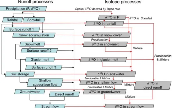
We then extended the WASA model for the simulation of the water isotopic composition of streamflow. Fig. 3 shows a schematic re-presentation of the extended model structure. We integrated the si-mulation of theδ-notion (‰) of18O into the WASA hydrological model
structure (hereafter abbreviated as IsoWASA model). We simulated the δ18
O signature instead ofδ2H in the model because the higher precision of theδ18O measurements ( ± 0.25‰) compared to the δ2H ( ± 0.4‰)
in our laboratory and both signatures are strongly correlated. Theδ18O
of streamflow was simulated by two modules: the initialization module ofδ18O inputs for water sources and the fractionation-mixing module of theδ18O of various runoff components along with the runoff generation
processes.
For the initialization ofδ18O inputs, we assumed thatδ18O of pre-cipitation, glacier melt and initial groundwater are linearly related to basin elevation (Allen et al., 2018). The elevation effect on isotopic
compositions of runoff components has been reported in previous stu-dies. For example, the elevation-gradient for precipitation isotopic composition was measured in the Himalaya areas byDalai et al. (2002). Field data in areas in the Central Andean measured byOhlanders et al. (2013)demonstrated the elevation effect on the isotopic composition of snowmelt. The δ18O value of glacier ice-melt water generated from
higher elevations tended to be more depleted in the Himalaya foothills, as measured byMaurya et al. (2011).Mark and McKenzie (2007)used an elevation-gradient to estimate the isotopic compositions of glacier melt dominated streamflow in an Andean sub-basin. Measurements from spring samples in a Greece mountain basin showed thatδ18O of groundwater decreased with the elevation increase (Payne et al., 1978). Based on the sampling data in our study basin, we estimated the elevation-gradients for the isotopic compositions of precipitation, gla-cier meltwater and groundwater inTable 1. The elevation-gradient for
Table 1
Summary of the characteristics ofδ18O and EC of various water samples. The coefficient of variation (CV) refers to the ratio between the standard deviation and mean value. The lapse rates forδ18O of precipitation (LPI), glacier melt (LGI) and initial groundwater (LGWI) were derived from the precipitation, glacier melt and winter streamflow samples.
Tracer Variable Sample number Mean Range CV
δ18O (‰) Streamflow at Baitik 158 −11.32 (−12.37, −10.82) 0.03 Streamflow at Alplager 184 −11.73 (−12.90, −10.94) 0.03 Precipitation at Baitik 36 −11.21 (−20.99, 1.51) 0.53 Precipitation at Alplager 43 −11.41 (−22.82, −0.06) 0.51 Groundwater 14 −11.17 (−11.70, −10.61) 0.03 Snowmelt 45 −13.98 (−24.24, −10.53) 0.26 Glacier melt 17 −13.46 (−15.66, −12.33) 0.08 LPI (‰/100 m) – −0.530 – – LGI (‰/100 m) – −0.226 – – LGWI (‰/100 m) – −0.210 – –
Electrical Conductivity (EC,μs/cm) Streamflow at Baitik 25 114.7 (81.0, 139.3) 0.13
Streamflow at Alplager 78 108.7 (66.7, 137.1) 0.18 Precipitation at Baitik 14 69.9 (26.6,99.6) 0.30 Precipitation at Alplager 23 68.3 (21.3,102.0) 0.30 Groundwater 12 126.8 (69.6, 167.2) 0.23 Snowmelt 7 28.4 (11.0, 55.1) 0.55 Glacier melt 3 32.1 (30.1, 33.4) 0.06
http://doc.rero.ch
the isotopic composition of precipitation (LPI) was estimated by the monthly isotope measurements at the Baitik (1580 m a.s.l.) and Al-plager (2100 m a.s.l.) meteorological stations. The elevation-gradient for the isotopic composition of glacier melt (LGI) was estimated by the isotopic compositions of summer samples fromflowing water on the Golubin glacier surface. The LGI was only applied in the ablation zone to calculate the isotopic composition of glacier melt. The elevation range of the ablation zone was defined as around 3200–4200 m a.s.l., according to ourfield investigations in summer. The isotopic compo-sition of glacier ice in the accumulation zone was not considered in this study. Regarding the isotopic composition of groundwater, we assumed that streamflow in January was fed by groundwater alone, which is the release of subsurface water storage recharged by runoff components in the warm season. Baseflow draining to the streamflow was defined as groundwater in this study basin. The elevation-gradient for the isotopic composition of groundwater (LGWI) was estimated by the January streamflow isotopic compositions measured at the Baitik and Alplager stations. To be noted, the LGWI was only used for the initialization of the groundwater isotopic composition in January when the model starting to run. The isotopic composition of groundwater was updated
daily in the model along with the generation and infiltration of surface runoff components. The elevation range to apply the LGWI was set as 1580–3200 m a.s.l., since 3200 m is the lowest elevation of the gla-cierized area in the basin. The terrain at altitudes higher than 3200 m a.s.l. is extremely steep in the study basin. Soil layers in these areas are very shallow. Contribution of groundwater from these areas is therefore assumed minor. The isotopic composition of subsurface runoff at alti-tudes higher than 3200 m are dominated by the isotopic compositions of rainfall and melt water.
The assumptions for fractionation-mixing ofδ18O of different runoff
components are as follows.δ18O of snowfall and rainfall were assumed
to be the same as that of precipitation. The changes in water isotopic composition caused by the rain out and snowfall out processes were not considered in the model. The initial snowpackδ18O was estimated as
theδ18O of thefirst snowfall in the modeling period. δ18O of snowpack accumulation (δ18O
SW) was then updated by the mixing ofδ18O of new
snowfall andδ18O of the existing snowpack.δ18O offlowing water on
snowpack surface was a mixture of theδ18O of snowmelt and potential rain on snow.δ18O of snowmelt (δ18O
SM) was simulated by a Rayleigh
fractionation method given in Eq.(1)(Hindshaw et al., 2011).δ18O of Fig. 2. EC measurements from water samples collected during the study period.
Table 2
Model parameters calibrated in all the four calibration methods.
Parameter Unit Value range Description
Snowmelt factor mm/°C/day 0–5 Degree-day factor for snowmelt
Glacier melt factor mm/°C/day 5–20 Degree-day factor for glacier melt
k_sat_f – 0.01–300 Soil hydraulic conductivities
kf_corr_f – 0.01–300 Soil hydraulic conductivities correction factor
frac2gw – 0–1 Recharge fraction factor from shallow subsurfaceflow to groundwater
Interflow delay factor days 0–100 Outflow delay factor for shallow subsurface flow
Groundwater delay factor days 30–400 Outflow delay factor for groundwater
frac_riparian – 0–0.05 Fraction of saturated area
sat_area_var – 0–0.3 Spatial variability of saturated areas within a model unit
p_correct_f – 0.0–2.0 Precipitation correction factor
the remaining snowpack (δ18
OSR) was then updated by the melt-out
δ18O of the snowmelt (Eq.(2)). The Rayleigh fractionation factor (α)
was assumed to be a function of temperature (Eq.(3), see alsoMajoube, 1971; Wolfe et al., 2007). A correction factor (CFs, Eqs.(1) and (2)) for
the fractionation factor was adopted to improve the simulation of the snowmeltδ18O. = + − − − − + δ O δ O f f ( 1000)·1 1 1000 SM SW CF α 18 18 s(1/ 1) 1 (1) = + − − δ O18 SR (δ O18 SW 1000)·fCFs·(1/α 1) 1000 (2) = − + − + α T T ln 0.00207 0.4156 11372 (3) = − f SM SW 1 (4) where SM is the out water amount generated by snowmelt, SW is the original snow water equivalent (SWE) in the snowpack, and SR is the remaining SWE after the snowmelt. f is the ratio of the remaining SWE to the original SWE in the snowpack. T (K) is the air temperature in the corresponding model spatial unit.
Theδ18O of direct runoff was derived from the mixing of δ18O of
rainfall, snowmelt, glacier melt and shallow subsurfaceflow (Fig. 3). δ18O of glacier meltwater at specific elevation band was calculated by
the LGI and meltwaterδ18O measured at the glacier tongue. Theδ18O of
shallow subsurfaceflow was updated by the mixing of the δ18O of the
infiltrated water from rainfall and meltwater and the δ18
O of existing soil water.δ18O of soil water was initialized as the δ18O of thefirst
infiltrated melt or rain water in the model period, and then updated by theδ18O of the infiltrated water and modulated by the evaporation process. Rayleigh fractionation processes inδ18O caused by evaporation in surface runoff and soil water storage were similarly considered by Eqs.(1)–(4). We adopted another correction factor (CFe) for the
eva-poration fractionation. Theδ18O of groundwater was derived by the mixing of initialδ18O of groundwater and theδ18O of the percolated
soil water storage. Finally, theδ18O of river streamflow was derived
from the mixing ofδ18O of direct runoff and groundwater outflow.
3.2. Model calibration
The calibration procedure for the IsoWASA model was implemented in four methods: (1) a benchmark single-dataset calibration using only discharge (observed at the Baitik station, same for the following), (2) a bi-dataset calibration using discharge andδ18O of streamflow, (3) a
tri-dataset calibration using discharge, MODIS snow cover area (SCA) and GMB, and (4) a four-dataset calibration based on the tri-dataset cali-bration used additionallyδ18O of streamflow. The bi-dataset calibration
was carried out to investigate the power of theδ18O of streamflow to
constrain the simulations of snow and glacier dynamics in comparison to the single-dataset calibration. The four-dataset calibration was used to test the benefits of the additional use of streamflow δ18O to reduce
parameter uncertainty, in comparison to the tri-dataset calibration. The model was evaluated at the daily time step for discharge, and at time steps according to the sampling interval for the other variables.
The model parameters calibrated in all the four calibration methods are summarized inTable 2. Initial values of the calibrated and non-calibrated parameters were adopted from He et al. (2018). For the fairness of comparison of the calibration methods, the correction factors CFsand CFefor water isotope fractionation were estimated prior to the
assessment of the four calibration methods, because these two factors have no effects on the performance of the single- and tri-dataset cali-bration methods. We first calibrated all the model parameters, in-cluding the correction factors CFsand CFe, only on the simulation of
streamflow δ18O. The calibrated values of CF
sand CFewere thenfixed
in the four calibration methods at 1.46 and 2.13, respectively. The multiple-objective ɛ-NSGAII automatic algorithm (Deb et al., 2002; Kollat and Reed, 2006) was run for the optimization of parameter va-lues in all the four calibration methods, with initial population size of eight and maximum number of function evaluations of 40,000. The average value of Nash–Sutcliffe efficiency (NSE, Eq. (5)) and loga-rithmic NSE (logNSE, Eq. (6)) was used as the objective function to evaluate the simulation of discharge (hereafter abbreviated as avNSE), the root mean squared error (SE, Eq.(7)) for the simulations of SCA and δ18O of streamflow, and the volumetric deviation efficiency at elevation
bands (VE, Eq.(8)) to assess the simulation for the GMB. The different
observation datasets were weighted equally by using the same Epsilon values in theɛ-NSGAII algorithm for the different objective functions.
Fig. 3. Schematic representation of the isotope-hydrological integrated modeling approach.
Since the streamflow isotope data is only available from July 2013, we selected the years 2015–2016 as the calibration period, and 2013–2014 as the evaluation period. The model was warmed up using two-year data before the calibration. In each calibration method, the model was run for four years. Thefirst two-year warm-up run was used to update the initial variable estimates. The values of model parameters were optimized based on thefitness between the simulated and observed datasets in the last two years. Forcing data in thefirst two years were simply repeated from the last two years in each calibration method. To identify the behavioral parameter sets from the Pareto-optimal fronts generated by theɛ-NSGAII algorithm in each calibration method, we defined acceptable threshold values for the performance metrics for the four observation datasets. For the simulation of discharge, we defined the acceptable threshold value for the avNSE metric as 0.8. The threshold values for SE and VE values for the simulations ofδ18O, SCA
and GMB were defined as 0.8, 0.8 and 0.95, respectively. In calibration methods that involved multiple observation datasets for the parameter optimization, only the parameter sets which produced performance metrics higher than the defined threshold values for all the observation datasets were identified as behavioral. The choices of the threshold values do not affect the conclusions, as the same threshold values were used for all the four calibration methods.
= − ∑ − ∑ − = = NSE Q i Q i Q i Q for discharge 1 ( ( ) ( )) ( ( ) ¯ ) , i n obs sim i n obs obs 1 2 1 2 (5) = −∑ − ∑ − = = NSE Q i Q i Q i Q for discharge
log 1 (log ( ) log ( ))
(log ( ) log ¯ ) , i n obs sim i n obs obs 1 2 1 2 (6) = − ∑= − SE S k S k
m for SCA and Isotope
1 k ( ( ) ( )) , m obs sim 1 2 (7) = − ∑ ∑ − ∑ ∑ = = = = VE M t M t M t for GMB 1 ( ( ) ( )) ( ) , t N l NB obsl siml t N l NB obsl 1 1 1 1 (8)
where Qobs(i) and Qsim(i) are the observed and simulated discharge on
day i, respectively;Qobs is the average observed daily discharge during the calibration period with n days; Sobs(k) and Ssim(k) are the
remotely-sensed and simulated SCA (or analyzed and simulatedδ18O of stream-flow) over the basin on day k, respectively; m is the total number of measured SCA (orδ18O) data used for the calibration during the
cali-bration period; Mlobs(t) and Mlsim(t) are the observed and simulated GMB
(mm) on the Golubin glacier at elevation band l in year t, respectively; NB is the total number of elevation bands, and N is the total number of the evaluated years.
3.3. Quantifying contributions of runoff components to streamflow using the isotope-hydrological integrated model and a tracer-based mixing method
The contributions of runoff components to the streamflow were quantified by two approaches in this study. We first estimated the contributions of runoff components with a tracer-based mixing method using measurements of water stable isotopic compositions and EC. The adopted three-component tracer conservative mixing method with rainfall, meltwater and groundwater as end members is described in Eq.
(9). Since the water tracer characteristics of snowmelt and glacier melt were very similar during the investigated periods, these two runoff components were treated as one component. We only used theδ18O
measurements for the mixing method, due to the high correlation be-tweenδ18O andδ2H. To consider the spatial variability in the rainfall δ18O, we used the volume-weighted average rainfall δ18O across the
basin instead of the measured precipitationδ18O at the meteorological
stations. The spatial distribution of rainfall was estimated by the lapse rates of precipitation and temperature. The spatial distribution of pre-cipitationδ18O was estimated by the elevation-gradient LPI.
Stream-flow δ18
O measured at the two meteorological stations were used for
the mixing method. Groundwater samples collected from the sampled spring were used in the tracer-based mixing method. The stream water samples in January were only used for the initialization of the groundwater isotopic composition in the hydrological model. The un-certainty in the mixing method was estimated by an error propagation method adopted inGenereux (1998) and Phillips and Gregg (2001).
⎧ ⎨ ⎪ ⎩⎪ = + + = + + = + +
Q RF GW MW for water balance
δ O Q δ O RF δ O GW δ O MW for δ O EC Q EC RF EC GW EC MW for EC , · · · · , · · · · , q RF GW MW q RF GW MW 18 18 18 18 18 (9) where RF refers to the runoff generated by rainfall, GW stands for the runoff generated by groundwater and MW is the total meltwater gen-erated by snowmelt and glacier melt.
Second, we estimated the contributions of runoff components based on the IsoWASA model outputs produced by the four calibration methods. The total simulated streamflow was first separated into two parts, i.e. groundwater and direct runoff. Direct runoff here is com-posed of the shallow subsurface flow and surface runoff triggered by rainfall and meltwater (Fig. 3). The groundwater storage was recharged by the percolation of shallow subsurfaceflow using the fraction factor frac2gw (Table 2), and the groundwater outflow was simulated by the
groundwater delay factor. The contribution of groundwater was di-rectly estimated as the ratio between the simulated groundwater and the total simulated streamflow. Direct runoff was estimated by sub-tracting the groundwater contribution from the total simulated streamflow, and was further assigned into three parts based on the proportions of the simulated runoff components (i.e. snowmelt, glacier melt and rainfall). Glacier melt was defined as melt from the glacier ice in this study.
The comparison of the quantification of runoff components pro-duced by the IsoWASA model and the tracer-based mixing method was carried out for two summer peakflow periods, because the snow and glacier melt runoff contribute the largest portion to streamflow in summer. The selected peakflow 1 extends from July 13th to August 19th 2015, and peakflow 2 from July 10th to August 10th 2016. As snow and glacier melt samples were not available during the period of peakflow 1, the δ18O and EC values for snow and glacier melt during
this peakflow were adopted from the samples during the period of peak flow 2. Snowmelt and glacier melt during the two peak flow periods should occur in similar elevation range in the two contiguous years. We assumed that the glacier melt water occurring at the same elevation band have similar water tracer characteristics. This assumption is supported by field data reported in other glacierized basins. For ex-ample, the sampling data in an Italian glacierized basin collected by
Penna et al. (2017) demonstrated that the isotopic compositions of glacier melt in two contiguous years are rather similar, and the EC in glacier meltwater showed low variability in space and time. Sampling data in the Himalaya foothills used byMaurya et al. (2011)showed that glacier melt occurred at the same latitude and altitude tended to have similar isotopic compositions. For snowmelt that occurred in the two peakflow periods, we assumed they presented the similar water tracer characteristics also because the water tracer characteristic of summer snowmelt was related to that of snowpack which was formed by snowfall in the last winter during the study period. Some carryover effect can be expected. Our field data show that the winter precipitation in the years of 2014 and 2015 have rather similar isotopic compositions and EC values (see alsoFigs. 2 and 8b and f).
Good model performance for the simulation of the peakflows is a prerequisite for the quantification of contributions of runoff compo-nents to the peak streamflow. However, hydrological models often failed to capture summer peakflows in high-elevation mountain basins (Aizen et al., 2000; Jasper et al., 2002; He et al., 2017), partly due to the incorrect climate inputs derived from the sparse climatic gauge stations (Li and Williams, 2008). Correcting the precipitation input for
hydrological modeling in high elevation glacierized basins has been commonly reported in previous studies (e.g.,Duethmann et al., 2013; Immerzeel et al., 2015). We thus added a precipitation (CP) and a
temperature (CT) correction factor to adjust the model inputs in the two
peakflow periods. We corrected both the precipitation and temperature inputs to (1) compare the performance of various calibration methods to correct the model inputs based on the constraints of various ob-servation datasets; (2) evaluate the ability of various calibration methods to reduce the compensation between temperature-triggered glacier melt runoff and precipitation-triggered runoff during the summer peakflow periods. The model parameters and the two addi-tional correction factors were recalibrated in the whole calibration period to obtain high performance for the simulation of the two peak flows.
4. Results
4.1. Model calibration and evaluation
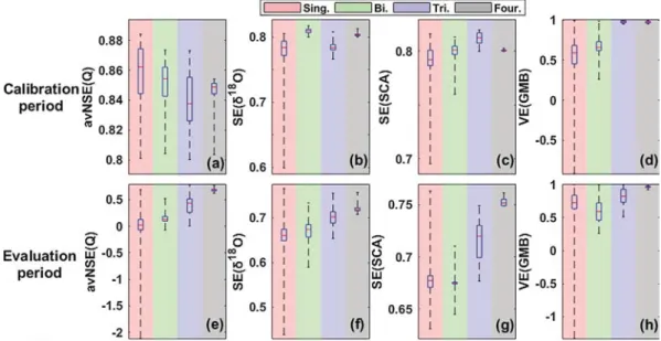
The values of the objective functions for the four observation da-tasets produced by the behavioral parameter sets in both calibration and evaluation periods are compared inFig. 4andTable 3. In the ca-libration period, the single-dataset method produced the highest per-formance for the simulation of discharge (median avNSE value is higher than 0.86,Fig. 4a andTable 3), while producing lower performance for the simulations of δ18O, SCA and GMB (see SE and VE values in
Fig. 4b–d and Table 3). The bi-dataset method yielded the highest performance for the simulation ofδ18O (Fig. 4b), while producing lower
performance for the simulation of GMB compared to the tri- and four-dataset methods (Fig. 4d). The tri-dataset method produced the highest performance for the simulations of SCA and GMB, while tending to produce SE values lower than 0.8 for the simulation ofδ18O. The four-dataset method produced high performance for the simulations ofδ18O and GMB, despite of its lower performance for the simulation of dis-charge than the single-dataset method and the lower performance for SCA than the tri-dataset method.
In the evaluation period (Fig. 4e–h andTable 3), the model per-formance for the four observation datasets tended to increase with in-creasing observation data involved in the calibration methods. For ex-ample, the model performance for discharge produced by the multi-dataset calibration methods were higher than that produced by the calibration to discharge only (Fig. 4e). The four-dataset method pro-duced the highest performance for all the four observation datasets in
terms of the median values of the objective functions, followed by the tri-dataset method.
Fig. 5shows the uncertainty ranges for the simulations produced by the behavioral parameter sets of the four calibration methods in the calibration period (similar situation in the evaluation period, not shown for the sake of brevity). The single-dataset calibration produced the largest uncertainty ranges, followed by the bi-dataset calibration. The four-dataset calibration generally produced the narrowest simulation ranges. The bi-dataset calibration reduced the uncertainty for the si-mulations of SCA and GMB compared to the single-dataset calibration (Fig. 5e–f and m–n), even though the information of SCA and GMB was
not used in this calibration approach. The additionally usedδ18O in the
bi-dataset calibration helped to constrain the simulations of SCA and GMB. The tri-dataset calibration method narrowed the uncertainty for the simulation of streamflow δ18
O compared to the single-dataset ca-libration method (Fig. 5i and k), despite theδ18O data was not used.
This can be explained by the fact that the dynamics of isotopic
Fig. 4. Values of objective functions for observation datasets produced by four calibration methods in the calibration (a–d) and evaluation (e–h) periods. Table 3
Summary of the model performance produced by four calibration methods.
Sing. Bi. Tri. Four.
Calibration period avNSE(Q) Max 0.8842 0.8736 0.8732 0.8541 Median 0.8623 0.8542 0.8376 0.8489 Min 0.8009 0.8041 0.8002 0.8035 SE(δ18O) Max 0.8057 0.8174 0.8080 0.8130 Median 0.7839 0.8100 0.7838 0.8034 Min 0.5993 0.8001 0.7663 0.8002 SE(SCA) Max 0.8164 0.8134 0.8199 0.8028 Median 0.7923 0.8013 0.8127 0.8010 Min 0.6955 0.7600 0.8001 0.8000 VE(GMB) Max 0.9969 0.9884 0.9999 0.9993 Median 0.5913 0.6607 0.9804 0.9802 Min −0.9163 0.2606 0.9501 0.9523
Evaluation period avNSE(Q) Max 0.6911 0.5217 0.7866 0.7683
Median 0.0219 0.1345 0.4353 0.6888 Min −2.1203 −0.0716 0.0071 0.6202 SE(δ18O) Max 0.7662 0.7337 0.7554 0.7576 Median 0.6609 0.6745 0.7023 0.7187 Min 0.4385 0.5898 0.6542 0.7080 SE(SCA) Max 0.7634 0.7104 0.7493 0.7616 Median 0.6773 0.6753 0.7200 0.7519 Min 0.6312 0.6450 0.6768 0.7490 VE(GMB) Max 0.9992 0.9980 0.9996 0.9879 Median 0.7285 0.5940 0.8231 0.9660 Min −1.3324 0.2606 0.5110 0.9237
http://doc.rero.ch
composition of streamflow are typically dominated by the snow and glacier melt runoff in glacierized basins.
4.2. Parameter uncertainty and identifiability
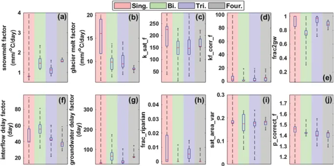
Fig. 6 shows the uncertainty ranges related to the values of the behavioral parameters calibrated by the four methods. The single-da-taset calibration produced the largest uncertainty ranges for all the ten parameters. The bi- and the tri-dataset calibrations narrowed the parameter ranges compared to the single-dataset calibration. It is worth noting that the bi-dataset calibration narrowed the uncertainty ranges for five parameters even stronger than the tri-dataset calibration
(Fig. 6c–d and h–j), even though only two datasets were involved in this
calibration method. The four-dataset calibration generally produced the smallest uncertainty ranges for all the parameters. This underscores the additional power of water isotopic data to constrain model parameters.
Fig. 7examines the sensitivity of the model performance for the simulation of the streamflow δ18O to the individual parameter values.
In each subplot, the model performance was tested on the value range of one specific parameter. The values for the other remaining para-meters were fixed using the optimized values from the four-dataset calibration. In terms of the curve slopes (see also the third column of
Table 4), the simulation of the streamflow δ18O shows the strongest sensitivity to the values of the snowmelt melt factor (Fig. 7a), followed
Fig. 5. Simulation ranges produced by the behavioral parameter sets of the four calibration methods in calibration period.
Fig. 6. Uncertainty ranges of the behavioral parameter sets produced by the four calibration methods.
by the values of parameters groundwater delay factor and p_correct_f (Fig. 7g and j). The SE value for the streamflow δ18O also shows
sig-nificant sensitivity to the parameters controlling the generation of di-rect runoff (e.g., parameters kf_corr_f and sat_area_var inFig. 7d and i) and glacier melt (Fig. 7b). These can be expected, as the dynamics in δ18
O signature are controlled by the dominance of snowmelt and gla-cier melt runoff, as well as the partitioning between direct runoff and groundwater. The parameter values that produced SE value higher than 0.8 for the simulation ofδ18O are assumed behavioral and labeled in red inFig. 7 (the normalized behavioral ranges are summarized in
Table 4). Data show that the δ18O data has varied power for
con-straining the behavioral ranges of model parameters, with the highest identifiability on the behavioral values of parameters snowmelt factor, kf_corr_f and p_correct_f (Fig. 7a, d and j).
4.3. Simulations ofδ18O of runoff components
Fig. 8 compares the simulated and measured δ18O of runoff
components in both calibration and evaluation periods. The simulated δ18O series were produced by the four-dataset calibration method using
the behavioral parameter sets. Fig. 8a and 8e present the simulated δ18O of groundwater in the model unit where the sampled spring is
located. The simulated groundwater δ18O are generally stable
throughout the year, apart from the slight increase in the summer months caused by the increased temperature. The simulated ground-waterδ18O tend to match the measured values well in the years 2015
and 2013 (Fig. 8a and e), while showing certain difference from the
measured values in July-August of 2016 and in August-September of 2014. Measured groundwaterδ18O in the years 2016 and 2014 show
large variability, partly because some of these samples were collected on rainy days. The sampled water from the spring on rainy days could be a mixture of groundwater and rainwater, leading to the abnormal δ18O measurements.
Fig. 8b and f shows the simulated and measured rainfallδ18O in the calibration and evaluation periods, respectively. Given the rainfallδ18O
in the model units was estimated by the LPI based on site measurements
Fig. 7. Sensitivity of the simulation performance of streamflow δ18O to individual parameter values.
Fig. 8. Seasonality of simulatedδ18O of various runoff components produced by the four-dataset calibration.
of precipitationδ18O, we presented the rainfallδ18O in all the model spatial units across the basin. Both the simulated and measured rainfall δ18O reach the highest values in the warm season and the lowest values
in the cold season. The simulated rainfallδ18O ranges generally capture the measured values in both calibration and evaluation periods. Be-cause the two meteorological stations, where precipitation samples were collected, are both located in the downstream area of the basin, the simulated rainfallδ18O in most model units appears to be lower
than the measured rainfallδ18O due to the elevation effect.
Fig. 8c–d and g–h presents the simulated and measured snowmelt
and glacier meltδ18O on the days when samples were collected. Only the simulatedδ18O of meltwater in the model units, where the sampled
sites are located, were presented. In the spring months of 2016 and 2014, the simulated snowmeltδ18O generally matched well with the measurements. However, in the spring months of 2015 and August of 2016, the simulated snowmeltδ18O are lower than the measurements
partly caused by the errors in the simulations of snow accumulation and melt processes. The simulated glacier meltδ18O tend to match the
measurements well in both the calibration and evaluation periods (Fig. 8d and h). To be noted, the IsoWASA model was not calibrated on the simulations of δ18O of runoff components. Only the δ18O of
streamflow was used in the model calibration procedure.
4.4. Contributions of runoff components quantified by different calibration methods
Fig. 9compares the contributions of runoff components at annual
and seasonal scales quantified by the four calibration methods in the calibration period. The uncertainty ranges of the contributions were caused by the uncertainty in the behavioral parameters inFig. 6.
At the annual scale (uncertainty ranges based on the four-dataset calibration), the runoff contributions to streamflow during the cali-bration period were 13.1–18.1% from rainfall (Fig. 9a), 17.6–24.7%
from snowmelt (Fig. 9f), 15–21.5% from glacier melt and 35.8–53.8% from groundwater (Fig. 9k and p). Rainfall mostly contributed to streamflow in spring and summer (Fig. 9b–c), while contributing in
autumn and winter remained below 8% (Fig. 9d–e). Groundwater was
the largest runoff component in all seasons, with the highest con-tributions of 90% during winter and the smallest concon-tributions of 35.7% in summer (Fig. 9t and r, from median values of the four-dataset method). Snowmelt was estimated to be the second largest runoff component in spring (Fig. 9g, 33.8%) and autumn (Fig. 9i, 12.9%). Glacier melt was the second largest runoff component in summer with
contribution of 28.5% (Fig. 9m).
The most obvious differences between the different calibration methods were in the uncertainty ranges. The single-dataset calibration method generally generated the largest uncertainty ranges, which partly resulted in estimates that were not reliable due to their large uncertainty range (e.g. estimated contribution of glacier melt of 6–44.8% at the annual scale inFig. 9k, and estimated winter snowmelt contribution of 0.1–79% inFig. 9j). The four-dataset calibration method resulted in the smallest uncertainty ranges. The difference in the sea-sonal contributions of snowmelt and groundwater are also visible (Fig. 9g–j and q–t). The single-dataset calibration tended to produce the
lowest (highest) contributions of snowmelt (groundwater), while the four-dataset calibration tended to produce the highest (lowest) con-tributions of snowmelt (groundwater). It becomes clear that the poorly constrained model tries to compensate the lack of meltwater by the higher groundwater contribution.
4.5. Comparison of the modeled contributions of runoff component to estimates from a tracer-based mixing method for two summer peakflows
Fig. 10 shows theδ18O and EC values analyzed from the water samples during the two selected summer peakflows. As expected, the δ18O of snow and glacier meltwater are the most depleted, followed by
the δ18O of groundwater. The groundwater presents the highest EC value followed by the rainfall samples. Snowmelt samples present si-milarδ18O and EC characteristics to the glacier melt samples. It is noted
that theδ18O of snow and glacier melt samples show a high variability. The variability in snowmeltδ18O can be attributed to the fact that the
snow samples were collected at different depths from the snowpack. Samples collected from deeper snow layers tend to have more depleted δ18O values. The variability in glacier meltδ18O can be explained by the
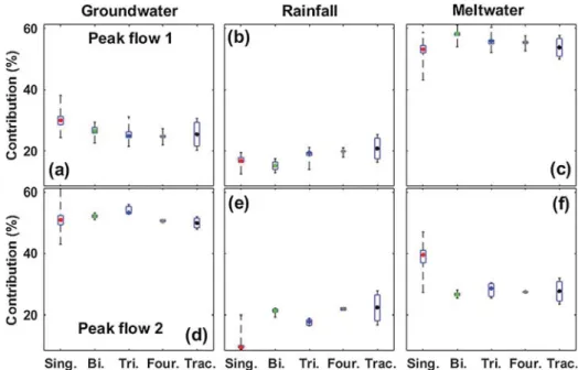
mixing of glacier melt water and potential snowmelt on glacier surface. The streamflow samples were perfectly located within the triangle areas formed by the runoff component samples. This provides a good basis for the tracer-based method to estimate the contributions of runoff com-ponents. The average values and the 95% confidence intervals for the contributions of individual runoff components estimated by the tracer-based method are presented inTable 5andFig. 11. The contributions show obvious uncertainty, especially for rainfall (Fig. 11b and e). Meltwater dominated the peakflow 1 with an average contribution of 54% (Fig. 11c), while groundwater dominated the peakflow 2 with an average contribution of 50% (Fig. 11d). Average contributions of rainfall during the two peakflows are both around 21%.
To estimate the contributions of runoff components based on the hydrological model output, we defined the behavioral parameter sets using the same threshold values for the performance metrics inSection 4.1, except the threshold value of avNSE for discharge which was set to 0.87 in this section to assure good performance for the reproductions of summer peakflows. The minimum/maximum and mean contributions of runoff components modeled by the four calibration methods are compared inFig. 11andTable 5. Generally, the four-dataset method produced the smallest uncertainties in the runoff components, while the single-dataset produced the largest uncertainties. The contribution ranges produced by the four-dataset method are generally located within the contribution ranges estimated by the tracer-based method. The single-dataset calibration method presents the largest deviations from the tracer-based method in both two peakflows. The different calibration methods resulted in significant differences in the mean contributions. For example, the single-dataset calibration method pro-duced the highest contribution of groundwater and the lowest con-tribution of meltwater in peakflow 1. The four-dataset method pro-duced the lowest contribution of groundwater (Fig. 11a). The bi-dataset method yielded the highest contribution of meltwater (Fig. 11c). The tri-dataset method estimated the meltwater contributions similarly to the four-dataset method, due to the dominance of snow and glacier melt runoff in this period. Snow and glacier observation data used in the
tri-Table 4
Summary of the sensitivity of the model performance for the simulation of streamflow δ18O to the model parameters. Width of behavioral range refers to the difference between the maximum and minimum normalized parameter values that produced SE (δ18O) value higher than 0.8. SEmax and SEmin stand for the maximum and minimum SE (δ18O) values produced by the individual parameters. Po represents the optimal normalized parameter value that pro-duced the highest SE (δ18O) value, and Pi represents the normalized parameter that produced a SE (δ18O) value as 0.8.
Parameter Width of behavioral
range
|(SEmax− SEmin)/(Po − Pi)|
Snowmelt factor 0.060 0.100
glacier melt factor 0.220 0.029
k_sat_f 0.858 0.004
kf_corr_f 0.071 0.021
frac2gw 0.128 0.012
Interflow delay factor 0.765 0.019
Groundwater delay factor 0.557 0.066 frac_riparian 0.216 0.007 sat_area_var 0.784 0.030 p_correct_f 0.062 0.050
http://doc.rero.ch
dataset method provide important information for the optimization of melt parameters. For peakflow 2 (Fig. 11d–f), the bi-dataset method
estimated the contributions similarly to the four-dataset method, partly due to the dominance of groundwater in this period. Theδ18O data used
in the bi-dataset method provided additional information on the
partitioning between direct runoff and groundwater.
In peakflow period 1, the single-dataset calibration overestimated (underestimated) the contribution of groundwater (meltwater) com-pared to the tracer-based method, which could be partly attributed to the overestimated (underestimated) precipitation (temperature) input
Fig. 9. Contributions of runoff components quantified by four calibration methods at annual and seasonal scales.
Fig. 10. Variability in the values ofδ18O and EC of water samples during the two summer peakflow periods.
(Fig. 12a and c). The single-dataset calibration estimated a negative CT
for the peakflow period 1 (Fig. 12c), and subsequently estimated a large CP to compensate the underestimated temperature input
(Fig. 12a). The four-dataset calibration method estimated the CTaround
0 °C (Fig. 12c–d) in both two peak flow periods, indicating the
tem-perature in high-elevation areas has likely been appropriately captured by the gauged temperature and lapse rate. In peakflow period 2, the single-dataset calibration method underestimated the contribution of rainfall compared to the tracer-based method (Fig. 11e), partly due to the underestimated precipitation input (Fig. 12b); and overestimated the contribution of meltwater (Fig. 11f), partly caused by the over-estimated temperature input (Fig. 12d). The contributions of runoff
components quantified by the bi- and tri-dataset calibration methods in
Fig. 11are generally consistent to the magnitudes of the precipitation and temperature inputs estimated by correction factors inFig. 12.
As expected, the four-dataset method helped to reduce the com-pensation between glacier melt (typically driven by temperature) and
precipitation-triggered runoff (i.e., sum of the rainfall and snowmelt runoff) during the peak flows as shown inFig. 13. The single-dataset method generally presents the most obvious compensation between the glacier melt and precipitation-triggered runoff indicated by the widest ranges for the quantifications of the runoff components, followed by the bi- and tri-dataset calibration methods. The simulated precipitation-triggered runoff and glacier melt runoff in peak flow 1 are larger than those in peakflow 2, due to that precipitation and temperature in the period of peakflow 1 were both higher than those in the period of peak flow 2. Results inFigs. 12 and 13demonstrate that the four-dataset calibration method performed well in correcting the model climate inputs and reducing the compensation between glacier melt and pre-cipitation-triggered runoff.
Table 5
Contributions (%) of three runoff components to streamflow quantified by various methods during two selected summer peakflows. Lower/upper limits refer to the 95% confidence intervals for the Tracer-based mixing method (Trac.), and refer to the minimum and maximum contributions produced by the behavioral parameter sets in the four calibration methods.
Sing. Bi. Tri. Four. Trac.
Peakflow 1 Groundwater Upper limit 38.1 29.4 31.1 27.3 30.6
Mean 30.0 26.7 24.9 24.7 25.4
Lower limit 24.3 22.6 21.5 21.9 20.2
Rainfall Upper limit 19.5 17.5 21.1 21.0 25.3
Mean 16.9 15.1 19.3 19.8 20.8
Lower limit 12.4 12.8 14.0 18.0 16.3
Meltwater Upper limit 58.7 61.1 60.4 57.6 57.6
Mean 53.1 58.2 55.8 55.5 53.8
Lower limit 43.1 54.0 52.1 52.6 49.9
Peakflow 2 Groundwater Upper limit 63 53.4 56.1 51.1 52.1
Mean 51 52.2 53.5 50.6 50.1
Lower limit 43 51.1 52.9 50.4 48
Rainfall Upper limit 19.9 22.1 19 22.3 27.8
Mean 9.5 21.3 17.9 22 22.3
Lower limit 8.7 19.4 16.5 21.4 16.8
Meltwater Upper limit 47.1 28 30.4 28 31.9
Mean 39.5 26.5 28.6 27.4 27.6
Lower limit 27.3 25.4 25.4 27.1 23.4
Fig. 11. Contributions of runoff components for the selected peak flows estimated by the four calibration methods and the tracer-based mixing model. Fig. 12. Estimated correction factors for precipitation and temperature inputs during the two peakflow periods by four calibration methods.
5. Discussions
5.1. Benefits of the water isotope data for hydrological modeling in glacierized basins
Comparisons between the single- and bi-dataset calibration methods indicate that involving the water isotope data for model calibration helped to improve the performance for the simulations of snow and glacier dynamics (Figs. 4 and 5). In glacierized basins where ground measured glacier mass balance data are not available, water isotope data bear the potential to provide constraint on the simulation of gla-cier melt runoff. The four-dataset calibration demonstrated the benefit of streamflow δ18
O to reduce the simulation uncertainty ranges in comparison to the dataset calibration. The performance of the tri-dataset method indicates that SCA and GMB data helped to constrain the simulation ofδ18O. This further indicates that the water isotopic composition of streamflow is capable of representing the dominance of snow and glacier melt during the summer months.
Compared to the other multi-dataset calibration runs, involving additional water isotopic compositions in the hydrological model cali-bration procedure further narrowed the uncertainty ranges in the quantification of runoff components. The compensations between runoff components were obviously reduced using the water isotopic compositions. The model parameters controlling the generation of groundwater can be identified well by the isotopic compositions, thus improving the constraining for the other remaining model parameters controlling the generations of rainfall and melt runoff. The water iso-topic compositions bear the potential to provide insights into the in-ternal apportionments of runoff components.
Our modeling results could also provide insights into the field sampling in glacierized basins. Weekly sampling from streamflow is prerequisite for the calibration of the isotope-hydrological integrated model. Monthly sampling for precipitation at two meteorological sta-tions seems appropriate to capture the spatial and seasonal variability of the isotopic composition of precipitation. Samples of glacier melt-water in summer from the ablation zone at different elevations are necessary for the initialization of isotopic composition of glacier melt. Taking stream water samples from sites with different elevations in January are required for the initialization of isotopic composition of groundwater in January. To apply the integrated modeling approach, water samples from snowmelt can be appropriately reduced, since the measurement of isotopic composition of snowmelt sample is not re-quired for the model initialization and calibration. To run the in-tegrated modeling approach in a short period, the sampling of glacier
melt water in the ablation area can be also appropriately reduced once the elevation-gradient of glacier melt isotope has been defined using sampling data during field campaigns, assuming the glacier melt iso-topic compositions are constant at specific locations in a short period. To improve the model performance, more sampling work could be spent on increasing sampling intervals for the streamflow and pre-cipitation. For example, more frequent sampling from streamflow over the day during the summer melt period could help to capture the diurnal cycle of the melt contribution. Using volume-weighted isotopic composition could provide more reliable estimates of the daily isotopic composition of streamflow. The sampling cost in high-elevation areas can be appropriately reduced. Our results show that the integrated modeling approach quantified the contributions of runoff components comparably to the tracer-based mixing method, and narrowed the un-certainty in the quantifications. Considering the requirement for larger sample sizes from various water sources in the end-member tracer-mixing approaches, the integrated modeling approach presents the superiority on quantifying runoff components based on less water tracer data.
5.2. Comparison with previous studies on tracer-aided hydrological modeling
Some previous studies developed tracer-aided hydrological models, including applications in snow-dominated basins. The performance of the IsoWASA model is comparable to the performance of these hydro-logical models, such as fromDelavau et al. (2017) and Ala-Aho et al. (2017b). Thefinding that water isotopic compositions helped to reduce model parameter uncertainty is consistent with that in Birkel et al. (2010) and Capell et al. (2012), who applied the tracer-aided hydro-logical model in two lowland catchments in Scotland.
For the simulation of the isotopic composition of snowmelt,Ala-aho et al. (2017a, 2017b)emphasized that sublimation from interception and ground snow storage, as well as the snowmelt fractionation could enrich the heavy isotopes in snowpack. In our study basin, the air hu-midity is typically high in the mountainous areas during the snow ac-cumulation period, and the snow interception by vegetation canopy is small due to the low vegetation coverage in winter; thus the sublima-tion effect on snow isotopes was not considered. We took into account the snowmelt fractionation effect to enrich the heavy isotopes in snowpack.Birkel et al. (2010) and Stadnyk et al. (2013)used the model proposed byCraig and Gordon (1965) to describe the effect of eva-poration fractionation on water isotopes. Considering the complex runoff mechanism in our glacierized basin, we simplified the
Fig. 13. Compensation between glacier melt and precipitation-triggered runoff during the two summer peak flow periods produced by different calibration methods.