HAL Id: halshs-00562645
https://halshs.archives-ouvertes.fr/halshs-00562645
Preprint submitted on 3 Feb 2011HAL is a multi-disciplinary open access
archive for the deposit and dissemination of sci-entific research documents, whether they are pub-lished or not. The documents may come from teaching and research institutions in France or abroad, or from public or private research centers.
L’archive ouverte pluridisciplinaire HAL, est destinée au dépôt et à la diffusion de documents scientifiques de niveau recherche, publiés ou non, émanant des établissements d’enseignement et de recherche français ou étrangers, des laboratoires publics ou privés.
Pessimism, Optimism and Credit Rationing
Jean-Louis Arcand
To cite this version:
Pessimism, Optimism and Credit Rationing
Jean-Louis Arcand
CERDI-CNRS, Université d’Auvergne,
and European Development Research Network
April 2, 2006
Abstract
In their celebrated contribution on credit rationing, Stiglitz and Weiss (1981) showed that the expected return to the borrower on a loan is increasing in the risk of the project it funds. In this paper, I show that their results do not necessarily carry over to the case where the agents’ preferences can be described by rank-dependent expected utility (RDEU). In particular, a pessimistic probability distortion function for borrowers can yield sufficient concavity in returns for the latter to be decreasing in risk, thus eliminating adverse selection. Whether credit rationing can obtain or not is then shown to depend upon the interaction between borrower pessimism and lender optimism.
Keywords: rank-dependent expected utility, credit rationing JEL: D81, D82
1
Introduction
In their celebrated article, Stiglitz and Weiss (1981) (henceforth, SW) showed that rationing could obtain in competitive credit markets as a result of adverse selection stemming from the inability of lenders to observe the riskiness of projects undertaken by borrowers. In this paper, I prove two results. First, if borrowers, whose preferences can be described by the rank-dependent expected utility (RDEU) model (Quiggin (1982)), are sufficiently pessimistic, then there may be no adverse selection in the market for loans because the Choquet expected return of a project to the borrower will not necessarily be an increasing function of its risk. Second, the Choquet average expected return of the loan to the lender can be a decreasing function of the interest rate, thereby rendering credit rationing possible, either (i) when borrowers are not overly pessimistic and lenders are not overly optimistic (an example being the standard expected utility (EU) case), or (ii) when borrowers are highly pessimistic and lenders are highly optimistic. In all other cases, the Choquet average expected return to the lender will be an unambiguously increasing function of the interest rate.
Both of these findings stand in contrast to two key aspects of the SW model of credit rationing, and show how its mechanics stem in part from the assumption that the preferences of agents can be adequately described by the EU model. Furthermore, the results presented here show that the manner in which risk is perceived by borrowers and lenders can potentially be an important, and hitherto neglected, determinant of the operation of the market for loans.
2
The standard result
Consider the standard SW model in which banks identify a pool of loan applicants who have projects with equal borrowing requirements D, and equal expected gross returns. While projects have identical mean returns, they differ in their riskiness. More precisely, a loan applicant in risk class ρ has a cumulative distribution function (cdf ) for gross returns θ ∈ [θ, θ] given by F (θ, ρ), where ρ is the Rothschild and
Stiglitz (1970) parameter of increasing risk and expected gross returns are denoted by μ =Rθθf (θ, ρ) dθ, where f (θ, ρ) = dF (θ,ρ)dθ . An increase in risk, as parameterized by ρ, is defined by the usual integral conditions: (i) Z θ θ Fρ(θ, ρ) dθ = 0, (ii) Z θ0 θ Fρ(θ, ρ) dθ> 0, ∀θ0∈ [θ, θ], (1) where ∂
∂ρF (θ, ρ) = Fρ(θ, ρ). In the absence of collateral possibilities, under the usual limited liability assumption, and given a gross interest rate i, the return to the borrower is eπ = max [θ − iD, 0]. The expected return to a loan applicant in risk class ρ is therefore:
Π(iD, ρ) = E [π] = Z θ iD(θ − iD) f (θ, ρ) dθ = θ − iD − Z θ iD F (θ, ρ) dθ, (2)
where the second equality follows by integration by parts. The key to the SW adverse selection result is that the expected return to the borrower is an increasing function of the risk ρ of the project, since:
∂Π(iD, ρ) ∂ρ = − Z θ iD Fρ(θ, ρ) dθ = Z iD θ Fρ(θ, ρ) dθ> 0, (3)
where the second equality follows from integral condition (1 (i)) and the inequality is a direct consequence of integral condition (1 (ii)). Mechanically, the result flows from eπ = max [θ − iD, 0] being convex in θ. Let ρ∗ be such that Π(iD, ρ∗) = K, where K is the borrower’s reservation level of return. Then, since ∂Π(iD,ρ)∂ρ > 0, only projects such that ρ > ρ∗ will be undertaken. By implicit differentiation of (2) evaluated at ρ∗: dρ∗ di = − ∂Π(iD,ρ∗) ∂i ∂Π(iD,ρ∗) ∂ρ∗ = D (1 − F (iD, ρ ∗)) RiD θ Fρ(θ, ρ∗) dθ > 0. (4)
Equation (4) is the SW adverse selection result: as the gross interest rate i increases, borrowers with low risk projects drop out of the market for loans, thereby increasing the average riskiness of the remaining projects faced by the lender. For the latter, the gross return on a loan is given by y = min [iD, θ]. The expected return to the lender is therefore:
Y (iD, ρ) = E [y] = Z iD θ θf (θ, ρ) dθ + Z θ iDiDf (θ, ρ) dθ = iD − Z iD θ F (θ, ρ) dθ, (5)
where the second equality follows from integration by parts. Differentiating (5) with respect to ρ and applying integral condition (1 (ii)) allows one to show that the lender’s expected return is decreasing in the riskiness of the project, ceteris paribus:
∂Y (iD, ρ)
∂ρ = −
Z iD θ
Fρ(θ, ρ) dθ6 0. (6)
Note also that ∂Y (iD,ρ)∂i = D [1 − F (iD, ρ)] > 0. Since the lender cannot directly observe which borrower undertakes the project, she must calculate an "average" expected return. Let ρ ∈ [ρ, ρ] be distributed in the population of borrowers according to the cdf H(ρ). Then the "average" expected return to the lender is given by:
Y (iD) = Rρ
ρ∗Y (iD, ρ)h(ρ)dρ
where h(ρ) = dH(ρ)dρ . Differentiating with respect to i and rearranging yields the standard SW expression: dY (iD) di = Rρ ρ∗D [1 − F (iD, ρ)] h(ρ)dρ 1 − H(ρ∗) + h(ρ∗) 1 − H(ρ∗) ¡ Y (iD) − Y (iD, ρ∗)¢ dρ∗ di . (8)
The first term in (8) is positive. The second term is negative because dρdi∗ > 0 by (4), while Y (iD) < Y (iD, ρ∗) since the expected return to the lender is greater on the "least risky" than on the "average" loan. Since Y (iD), Y (iD, ρ∗) and ρ∗do not depend upon h(ρ∗), the negative term can be made arbitrarily large in absolute value terms by choosing h(ρ∗) large. Thus, an increase in the gross interest rate reduces the lender’s average expected return from loans.
3
RDEU preferences
Let S = {s0, s1, ..., si, ..., sn} be the finite set of states of nature. Consider the set of subsets of S, denoted by E = 2S, which we shall refer to as the set of events. Let X : S → R with s → X(s). Then ν : A ∈ E → ν(A) ∈ [0, 1] is a capacity if ν(∅) = 0, ν(S) = 1, and A ⊆ B ⇒ ν(A) 6 ν(B); ν is convex if ν(A ∪ B) + ν(A ∩ B) > ν(A) + ν(B), ∀A, B ∈ E.
The Choquet (1953) integral of X with respect to ν is given by:
EC[X] = Z 0 −∞[ν ({X > x}) − 1] dx + Z ∞ 0 ν ({X > x}) dx. (9) By Theorem 7 in Wakker (1990), if the decisionmaker’s preferences are consistent with first-order sto-chastic dominance with respect to probability measure P , the capacity takes the form ν ({X > x}) = ϕ (P ({X > x})) = ϕ (1 − F (x)), where F (x) is the cumulative density function of X, and ϕ(.) is nonde-creasing with ϕ (0) = 0 and ϕ (1) = 1; ϕ (.) is unique and plays the role of a probability transformation function. As shown by Roell (1987), Demers and Demers (1990), and Guriev (2001), assuming that ϕ (.) is differentiable and integrating by parts then allows one to rewrite the Choquet expectation in (9) in terms of the Lebesgue-Stieltjes integral:
EC[X] = Z ∞
−∞
xϕ0(1 − F (x)) f(x)dx, (10)
where f (x) = dF (x)dx . The "distorted" expectation given in (10) corresponds to Yaari’s (1987) dual theory functional, and its differentiability has recently been studied by Carlier and Dana (2003). While one can take ϕ(.) to be a component of the agents’ risk preferences in a RDEU context, the results that follow can also be reinterpreted in terms of Choquet-Schmeidler expected utility (CEU, Gilboa (1987), Schmeidler (1989)), where a convex (concave) ϕ(.) corresponds to ambiguity aversion (preference).
For the case at hand, application of (10) yields the following expression for the Choquet expectation of the borrower’s return, where ϕ (.) is understood to be the borrower’s probability distortion function:
ΠC(iD, ρ) = EC[eπ] = Z θ iD(θ − iD) ϕ 0(1 − F (θ, ρ)) f (θ, ρ) dθ =Z θ iDϕ (1 − F (θ, ρ)) dθ, (11)
where the last equality follows from noting that dθd [−ϕ (1 − F (θ, ρ))] = ϕ0(1 − F (θ, ρ)) f (θ, ρ) and integrating by parts. When ϕ (x) = x, equation (11) boils down to the EU expression given in (2).
Let ρ∗∗ be such that ΠC(iD, ρ∗∗) = K. On the one hand, ∂ΠC(iD,ρ∗∗)
∂i = −Dϕ (1 − F (iD, ρ∗∗)). On the other, differentiating ΠC(iD, ρ∗∗) with respect to ρ∗∗, integrating by parts, applying integral condition (1 (i)), and assuming that ϕ0(0) is bounded from above, immediately yields the following
0 0.5 1 1.5 2 iD 0.5 1 1.5 ρ 0 0.5 1 πHiD,ρL 0 0.5 1 1.5 iD 0 0.5 1 1.5 2 iD 0.5 1 1.5 ρ 0 0.2 0.4 0.6 0.8 πCHiD,ρL 0 0.5 1 1.5 iD
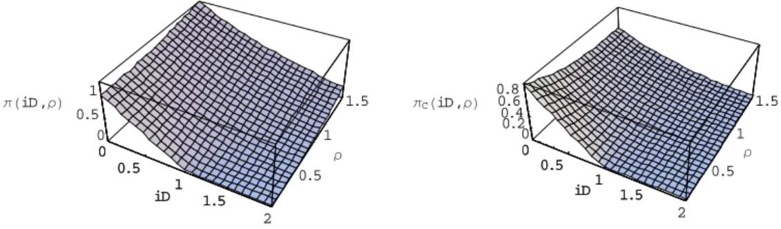
Figure 1: The expected return and Choquet expected return to the borrower as functions of iD and ρ. The right-hand panel represents ΠC(iD, ρ) for ϕ(x) = x2 and θ ∼ N(1, σ2). The left-hand panel represents the corresponding EU case (Π(iD, ρ)).
Proposition:
Proposition 1 Under RDEU preferences, the limit risk class ρ∗∗ is not necessarily increasing in the interest rate i: dρ∗∗ di = − ∂ΠC(iD,ρ∗∗) ∂i ∂ΠC(iD,ρ∗∗) ∂ρ =⎛ Dϕ (1 − F (iD, ρ∗∗)) ⎝ ϕ0(1 − F (iD, ρ∗∗)) ³RiD θ Fρ(z, ρ∗∗) dz ´ −RiDθ ϕ00(1 − F (θ, ρ∗∗)) f (θ, ρ∗∗) ³Rθ θ Fρ(z, ρ∗∗) dz ´ dθ ⎞ ⎠ .
The key difference between the EU and the RDEU cases is thus apparent: for ϕ(.) convex, dρdi∗∗ may be negative. The reason lies in the denominator of the expression given in the Proposition (∂ΠC(iD,ρ∗∗)
∂ρ ),
which is not necessarily positive, as for the EU case given in (4). Formally, this is because:
ϕ0(1 − F (iD, ρ∗∗)) ÃZ iD θ Fρ(z, ρ∗∗) dz ! > 0, (12)
since ϕ0(.)> 0 and RθiDFρ(z, ρ∗∗) dz> 0 by integral condition (1 (ii)), whereas:
− Z θ iD ϕ00(1 − F (θ, ρ∗∗)) f (θ, ρ∗∗) ÃZ θ θ Fρ(z, ρ∗∗) dz ! dθ6 0, (13) since ϕ00(.) > 0, f (θ, ρ∗∗)> 0, and Rθ
θ Fρ(z, ρ∗∗) dz> 0. The intuition for the result is straightforward: pessimism in the borrower’s probability distortion function can induce sufficient concavity in her objective function to overcome the convexity of eπ that lies at the heart of the SW result. In this case, it will be the high risk borrowers who will progressively drop out of the market for loans, and there will be no adverse selection. In the EU case, the term that includes ϕ00(.) vanishes and ϕ0(.) = 1, ensuring that the limit risk class ρ∗ is unambiguously increasing in the interest rate.
As an illustration, consider the parametric example in which ϕ (x) = x2 and θ ∼ N(1, σ2). For this illustration based on the normal density, ρ corresponds to the standard deviation σ. The right-hand panel of Figure 1 represents the RDEU case, whereas its EU counterpart (ϕ (x) = x) is represented on the left. Expected returns to the borrower are close to zero at iD ≈ 1 for low values of ρ because we have set E[θ] = μ = 1, which implies that EC[θ] = μ −√σπ. Π(iD, ρ) is unambiguously increasing in risk
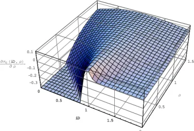
0 0.5 1 1.5 2 iD 0.5 1 1.5 ρ -0.3 -0.2 -0.1 0 0.1 ∂πC HiD, ρL ∂ ρ 0 0.5 1 1.5 iD Figure 2: ∂ΠC(iD,ρ) ∂ρ as a function of of iD and ρ.
in the left-hand panel (the standard SW result), while there are many configurations in the right-hand panel that yield a ΠC(iD, ρ) that is decreasing in ρ. Figure 2 provides a further illustration of the RDEU case by plotting ∂ΠC(iD,ρ)
∂ρ as a function of iD and ρ, under the same parametric assumptions. As should be clear, ∂ΠC(iD,ρ)
∂ρ becomes positive only once iD and ρ are sufficiently large.
Consider now the lender’s side. Denote the lender’s probability distortion function by φ(.). Applying (10) and integrating by parts yields the Choquet expectation of the lender’s return:
YC(iD, ρ) = θ + Z iD
θ φ (1 − F (θ, ρ)) dθ.
(14)
Differentiating with respect to ρ, integrating by parts, assuming that φ0(1) is bounded from above, and applying (1 (i)) yields the following Proposition:
Proposition 2 Under RDEU preferences, the expected return to the lender YC(iD, ρ) is not necessarily a decreasing function of the risk ρ of the project:
∂YC(iD, ρ) ∂ρ = −φ 0(1 − F (iD, ρ))ÃZ iD θ Fρ(z, ρ) dz ! − Z iD θ φ00(1 − F (θ, ρ)) f (θ, ρ) ÃZ θ θ Fρ(z, ρ) dz ! dθ.
Proposition 2 shows that, contrary to the EU case as given by (6), the Choquet expectation of the return to the lender is not necessarily a decreasing function of the riskiness of the project. Indeed, if the lender’s probability distortion function is sufficiently concave (i.e., if the lender is sufficiently optimistic), then the lender’s expected return to the project can be an increasing function of its riskiness. On the other hand, if the lender is pessimistic, one obtains the standard SW result since ∂YC(iD,ρ)
∂ρ will be negative. Note also that ∂YC(iD,ρ)
∂i = Dφ (1 − F (iD, ρ)) > 0.
pessimistic, as set out in Proposition 1, and therefore dρdi∗∗ > 0: YC(iD) = Rρ ρ∗∗YC(iD, ρ)φ0(1 − H (ρ)) h(ρ)dρ Rρ ρ∗∗φ0(1 − H (ρ)) h(ρ)dρ . (15)
Differentiating with respect to i yields: dYC(iD) di = Rρ ρ∗∗Dφ (1 − F (iD, ρ)) φ0(1 − H (ρ)) h(ρ)dρ Rρ ρ∗∗φ0(1 − H (ρ)) h(ρ)dρ (16) + φ 0(1 − H (ρ∗∗)) h(ρ∗∗) Rρ ρ∗∗φ0(1 − H (ρ)) h(ρ)dρ ¡ YC(iD) − YC(iD, ρ∗∗) ¢ dρ∗∗ di .
As in the EU case considered in (8), the second term is negative, as long as lenders are not overly optimistic (as spelled out in Proposition 2, so that ∂YC(iD,ρ)
∂ρ < 0) so that YC(iD) < YC(iD, ρ∗∗).1 Credit rationing may therefore obtain. On the other hand, if borrowers are sufficiently pessimistic so that dρdi∗∗ 6 0: YC(iD) = Rρ∗∗ ρ YC(iD, ρ)φ0(1 − H (ρ)) h(ρ)dρ Rρ∗∗ ρ φ0(1 − H (ρ)) h(ρ)dρ , (17)
where it is important to note that the limits of integration have changed, and: dYC(iD) di = Rρ∗∗ ρ Dφ (1 − F (iD, ρ)) φ0(1 − H (ρ)) h(ρ)dρ Rρ∗∗ ρ φ0(1 − H (ρ)) h(ρ)dρ (18) + φ 0(1 − H (ρ∗∗)) h(ρ∗∗) Rρ∗∗ ρ φ0(1 − H (ρ)) h(ρ)dρ ¡ YC(iD, ρ∗∗) − YC(iD) ¢ dρ∗∗ di .
Here, ρ∗∗ corresponds to the riskiest project and YC(iD, ρ∗∗) < YC(iD) if lenders are not overly opti-mistic (so that ∂YC(iD,ρ)
∂ρ < 0). The second term in (18) will then be unambiguously positive, as will dYC(iD)
di : no credit rationing can then obtain. The converse of the preceding two cases can be constructed for optimistic lenders for whom ∂YC(iD,ρ)
∂ρ > 0.
4
Concluding remarks
In this paper I have shown that the key adverse selection result of the SW model of credit rationing depends upon borrowers not being overly pessimistic, as this concept is defined in the RDEU model. If borrowers are particularly pessimistic, it will be the high risk group that will be the first to drop out of the market for loans, contrary to the usual SW result. The perception by lenders of the Choquet average expected return on their remaining pool of loan applicants determines whether credit rationing can obtain or not. If borrowers are sufficiently pessimistic so as to eliminate the adverse selection problem, pessimistic (or EU) lenders are sufficient to ensure that the Choquet average expected return to lenders will be unambiguously increasing in the interest rate. Conversely, if lenders are not pessimistic enough and adverse selection exists, sufficiently optimistic borrowers can also ensure that the Choquet average expected return to lenders is unambiguously increasing in the interest rate.
It is straightforward to show that all of the results presented here carry over to the case of collateral, as considered in Wette (1983). An important extension would be to study the existence of adverse
1The term φ0(1−H(ρ∗∗))h(ρ∗∗) Uρ
ρ∗∗φ0(1−H(ρ))h(ρ)dρ
selection in the SW model under RDEU preferences using richer notions of mean-preserving increases in risk such as those proposed by Chateauneuf, Cohen, and Meilijson (2004).
References
Carlier, G., and R. A. Dana (2003): “Core of Convex Distortions of a Probability,” Journal of Economic Theory, 113(2), 199—222.
Chateauneuf, A., M. Cohen,and I. Meilijson (2004): “Four Notions of Mean-Preserving Increase in Risk, Risk Attitudes and Applications to the Rank-Dependent Expected Utility Model,” Journal of Mathematical Economics, 40(5), 547—571.
Choquet, G. (1953): “Théories des Capacités,” Annales de l’Institut Fourier, 5, 131—295.
Demers, F.,andM. Demers (1990): “Price Uncertainty, the Competitive Firm and the Dual Theory of Choice under Risk,” European Economic Review, 34(6), 1181—1199.
Gilboa, I. (1987): “Expected Utility Without Purely Subjective Non-Additive Probabilities,” Journal of Mathematical Economics, 16(1), 65—88.
Guriev, S. (2001): “On Microfoundations of the Dual Theory of Choice,” The Geneva Papers on Risk and Insurance Theory, 26(2), 117—137.
Quiggin, J. (1982): “A Theory of Anticipated Utility,” Journal of Economic Behaviour and Organiza-tion, 3(4), 323—343.
Roell, A. (1987): “Risk Aversion in Quiggin and Yaari’s Rank-Order Model of Choice under Uncer-tainty,” Economic Journal, 97(Supplement: Conference Papers), 143—159.
Rothschild, M., and J. E. Stiglitz (1970): “Increasing Risk I: A Definition,” Journal of Economic Theory, 2(3), 225—243.
Schmeidler, D. (1989): “Subjective Probability and Expected Utility Without Additivity,” Economet-rica, 57(3), 571—587, first version 1982.
Stiglitz, J. E., and A. Weiss (1981): “Credit Rationing in Markets with Imperfect Information,” American Economic Review, 71(3), 393—410.
Wakker, P. (1990): “Under Stochastic Dominance Choquet-Expected Utility and Anticipated Utility are Identical,” Theory and Decision, 29(2), 119—132.
Wette, H. C. (1983): “Collateral in Credit Rationing in Markets with Imperfect Information: Note,” American Economic Review, 73(3), 442—445.