HAL Id: hal-02972968
https://hal.archives-ouvertes.fr/hal-02972968
Submitted on 20 Oct 2020
HAL is a multi-disciplinary open access
archive for the deposit and dissemination of
sci-entific research documents, whether they are
pub-lished or not. The documents may come from
teaching and research institutions in France or
abroad, or from public or private research centers.
L’archive ouverte pluridisciplinaire HAL, est
destinée au dépôt et à la diffusion de documents
scientifiques de niveau recherche, publiés ou non,
émanant des établissements d’enseignement et de
recherche français ou étrangers, des laboratoires
publics ou privés.
Numerical approximation and optimization of the
support
Arthur Bottois
To cite this version:
Arthur Bottois. Pointwise moving control for the 1-D wave equation - Numerical approximation and
optimization of the support. Radon Series on Computational and Applied Mathematics, De Gruyter,
In press. �hal-02972968�
wave equation
Numerical approximation and optimization of the support
Abstract:We consider the exact null controllability of the 1-D wave equation with an interior pointwise control acting on a moving point (𝛾(𝑡))𝑡∈(0,𝑇 ). We approximate a
control of minimal norm through a mixed formulation solved by using a conformal space-time finite element method. We then introduce a gradient-type approach in order to optimize the trajectory 𝛾 of the control point. Several experiments are discussed.
Keywords:exact controllability, wave equation, pointwise control, mixed formulation, finite element approximation
1 Introduction
Let 𝑇 > 0. We consider the linear one-dimensional wave equation in the interval Ω = (0, 1), with a pointwise control 𝑣 acting on a moving point 𝑥 = 𝛾(𝑡), 𝑡 ∈ [0, 𝑇 ]. The state equation reads
⎧ ⎪ ⎨ ⎪ ⎩ 𝑦𝑡𝑡− 𝑦𝑥𝑥= 𝑣(𝑡)𝛿𝛾(𝑡)(𝑥) in 𝑄𝑇 = Ω × (0, 𝑇 ), 𝑦 = 0 on Σ𝑇 = 𝜕Ω × (0, 𝑇 ), (𝑦, 𝑦𝑡)(·, 0) = (𝑦0, 𝑦1) in Ω. (1)
Here, 𝛿𝛾(𝑡) is the Dirac measure at 𝑥 = 𝛾(𝑡) and 𝛾 represents the trajectory in
time of the control point. The curve 𝛾 : [0, 𝑇 ] → Ω is assumed to be piecewise 𝐶1.
We also denote by H′ the dual space of H := 𝐻1
(0, 𝑇 ). For 𝑣 ∈ H′, we refer to Section 2.1 for the well-posedness of (1).
The exact null controllability problem for (1) at time 𝑇 > 0 is the following. Given a trajectory 𝛾 : [0, 𝑇 ] → Ω, for any initial datum (𝑦0, 𝑦1) ∈ V := 𝐿2(Ω) ×
𝐻−1(Ω), find a control 𝑣 ∈ H′ such that the corresponding solution 𝑦 of (1)
*Corresponding author: Arthur Bottois,Université Clermont Auvergne, Laboratoire de Mathématiques Blaise Pascal CNRS-UMR 6620, Campus des Cézeaux, F-63178 Aubière cedex, France, e-mail: [email protected]
satisfies
(𝑦, 𝑦𝑡)(·, 𝑇 ) = (0, 0) in Ω.
As a consequence of the Hilbert uniqueness method (HUM) introduced by J.-L. Lions [25], the controllability of (1) is equivalent to an observability inequality for the associated adjoint problem. Indeed, the state equation (1) is controllable if and only if there exists a constant 𝐶obs(𝛾) > 0such that
‖(𝜙0, 𝜙1)‖2W≤ 𝐶obs(𝛾)‖𝜙(𝛾, ·)‖ 2 H, ∀(𝜙0, 𝜙1) ∈ W := 𝐻01(Ω) × 𝐿2(Ω), (2) where 𝜙 ∈ 𝐶([0, 𝑇 ]; 𝐻1 0(Ω)) ∩ 𝐶1([0, 𝑇 ]; 𝐿2(Ω))solves 𝐿𝜙 = 0in 𝑄𝑇, 𝜙 = 0on Σ𝑇, (𝜙, 𝜙𝑡)(·, 0) = (𝜙0, 𝜙1)in Ω. (3)
Here, the notation 𝜙(𝛾, ·) stands for the function 𝜙(𝛾(𝑡), 𝑡) with 𝑡 ∈ (0, 𝑇 ), while 𝐿denotes the wave operator
𝐿 = 𝜕𝑡2− 𝜕𝑥2.
Under additional assumptions on 𝛾, a proof of (2) can be found in [8]. We emphasize that the observability constant 𝐶obs(𝛾)depends on the control trajectory 𝛾. In
what follows, we say that 𝛾 is an admissible trajectory if the observability inequality (2) holds true.
In this work, we investigate the issue of the numerical approximation of the control̂︀𝑣𝛾 of minimal H
′-norm and the associated controlled state. We also tackle
the problem of optimizing the support of control, which is done numerically by minimizing the norm ‖̂︀𝑣𝛾‖H′ with respect to the trajectory 𝛾.
Let us now mention some references related to pointwise control. This problem arises naturally in practical situations when the size of the control domain is very small compared to the size of the physical system. For a stationary control point 𝛾 ≡ 𝑥0∈ Ω, the controllability of (1) depends strongly on the location of
𝑥0 [24, 26, 14]. Indeed, one can show that controllability holds if and only if the
controllability time 𝑇 is large enough, i.e. 𝑇 ≥ 2|Ω|, and if there is no eigenfunction of the Dirichlet Laplacian vanishing at 𝑥 = 𝑥0. The constraint on 𝑇 is due to
the finite speed of propagation of the solution of the wave equation (1). A point 𝑥0 satisfying the previous spectral property is referred to as a strategic point.
Furthermore, 𝑥0is a strategic point if and only if it is irrational with respect to the
length of Ω, making controllability very unstable. Consequently, controls acting on stationary points are usually difficult to implement in practice. It is often more convenient to control along curves for which the strategic point property holds a.e. in [0, 𝑇 ].
For a moving control point 𝑥 = 𝛾(𝑡), several sufficient conditions to ensure controllability have been studied [20, 22, 8, 1]. In [22], the author proves the
existence of controls in 𝐿2(0, 𝑇 )acting on a point rapidly bouncing between two
positions. In [8, Proposition 4.1], the author shows, using the d’Alembert formula, that the observability inequality (2) holds under some geometric restrictions on the trajectory 𝛾. By duality, this implies the existence of controls in H′for initial
data in V. The geometric requirements are related to the usual geometric control condition (GCC) introduced for controls acting over domains 𝜔 ⊂ Ω [3, 23]. Among the constraints given to guarantee that 𝛾 is admissible, there must exist two constants 𝑐1, 𝑐2> 0 and a finite number of subintervals (𝐼𝑗)0≤𝑗≤𝐽 ⊂ [0, 𝑇 ]such
that, for each subinterval 𝐼𝑗, 𝛾 ∈ 𝐶1(𝐼𝑗), 1 − |𝛾′|does not change sign in 𝐼𝑗 and
𝑐1 ≤ |𝛾′| ≤ 𝑐2 in 𝐼𝑗. The constants appearing in the proof of the observability
inequality (2) depend only on 𝑐1 and 𝑐2(see [8, Remark 4.2]). Thus, it is possible
to write a uniform observability inequality for trajectories in a suitable class, i.e. there exists 𝐶 > 0 such that 𝐶obs(𝛾) ≤ 𝐶for every 𝛾 in that class.
In the context of feedback stabilization, we mention [2]. For parabolic equations, we also mention [26, 21]. Finally, for the computation of pointwise controls for the Burgers equation, we refer to [4, 31].
The main contributions of this paper are the following. First, we use the HUM method to characterize the control̂︀𝑣of minimal H
′-norm, also known as the HUM
control. We then turn our attention to the numerical approximation of this control and the associated controlled state. Usually (see [16, 29]), such an approximation is computed by minimizing the so-called conjugate functional 𝒥⋆
𝛾 : W →Rdefined by 𝒥𝛾⋆(𝜙0, 𝜙1) = 1 2‖𝜙(𝛾, ·)‖ 2 H− ∫︁ Ω 𝑦0𝜙1+ ⟨𝑦1, 𝜙0⟩−1,1, (4)
where 𝜙 is the solution of (3) associated with (𝜙0, 𝜙1), and ⟨·, ·⟩−1,1 stands for
the duality product in 𝐻1
0(Ω). Here, instead, we notice that the unconstrained
minimization of 𝒥⋆
𝛾(𝜙0, 𝜙1)is equivalent to the minimization of another functional
̃︀
𝒥𝛾⋆(𝜙)(cf. (17)) over 𝜙 satisfying the constraint 𝐿𝜙 = 0. This constraint is taken
into account using a Lagrange multiplier which leads to a mixed formulation where the space and time variables are embedded. We follow the steps of [13, 9], where a similar formulation is used for controls distributed over non-cylindrical domains 𝑞 ⊂ 𝑄𝑇. It is worth mentioning that this space-time approach is well-adapted to our
moving point situation, since we can achieve a good description of the trajectory 𝛾 embedded in a space-time mesh of 𝑄𝑇. From a numerical point of view, we build a
Galerkin approximation of the mixed formulation using conformal space-time finite elements. This allows to compute the optimal adjoint state𝜙̂︀, linked to the HUM
control𝑣̂︀by the relation (9). This also gives an approximation of the Lagrange
Another aspect of this work is the numerical optimization of the support of control. For a given initial datum (𝑦0, 𝑦1) ∈ V, we want to minimize the norm
‖̂︀𝑣𝛾‖H′ of the HUM control
̂︀
𝑣𝛾 with respect to the trajectory 𝛾. To do so, we
consider the functional
𝐽 (𝛾) = 1 2‖̂︀𝑣𝛾‖
2
H′ (5)
and we implement a gradient-type algorithm. In order to find a descent direction at each iteration, we establish a formula for the directional derivative of 𝐽. The values of 𝐽 are computed using the approximate control arising from the mixed formulation mentioned previously. We perform several numerical experiments and compare our results with those obtained in [6] for controls distributed over non-cylindrical domains 𝑞 ⊂ 𝑄𝑇. In the simulations, the admissible set of trajectories 𝛾
is discretized using splines functions of degree 5.
The rest of the paper is organized in three sections. First, in Section 2, we briefly give some theoretical results. Namely, we justify the existence of weak solutions for the state equation (1), and we characterize the control of minimal H′-norm
using the HUM method. We also analyse the extremal problem min𝛾𝐽 (𝛾)(cf. (5))
and compute the directional derivative of 𝐽 with respect to 𝛾. In a second step, in Section 3, we present the space-time mixed formulation used to approximate the control and the controlled state. We also discuss some issues related to the discretization of that formulation. Finally, in Section 4, we give several numerical experiments. We illustrate the convergence of the approximated control as the discretization parameter goes to zero. For stationary control points 𝛾 ≡ 𝑥0∈ Ω, we
illustrate the lack of controllability at non-strategic points. We also describe the gradient-type algorithm designed to optimize the support of control and discuss some results.
2 Some theoretical results
2.1 Existence of weak solutions for the state equation
The weak solution of (1) is defined by transposition (see [27]). For any 𝜓 ∈ 𝐿1(0, 𝑇 ; 𝐿2(Ω)), let 𝜙 ∈ 𝐶([0, 𝑇 ]; 𝐻01(Ω)) ∩ 𝐶1([0, 𝑇 ]; 𝐿2(Ω))be the solution of the
backward adjoint equation
Multiplying (1) by 𝜙 and integrating by parts, we formally obtain ∫︁ ∫︁ 𝑄𝑇 𝑦𝜓 = ⟨𝑣, 𝜙(𝛾, ·)⟩H′,H− ∫︁ Ω 𝑦0𝜙𝑡(·, 0)+⟨𝑦1, 𝜙(·, 0)⟩−1,1, ∀𝜓 ∈ 𝐿1(0, 𝑇 ; 𝐿2(Ω)), (6) where ⟨·, ·⟩−1,1 and ⟨·, ·⟩H′,Hdenote respectively the duality products in 𝐻01(Ω)
and H. We adopt identity (6) as the definition of the solution of (1) in the sense of transposition. One can then prove the following result (see [8, Theorem 2.1]). Lemma 1. Let 𝛾 : [0, 𝑇 ] → Ω be piecewise 𝐶1. If there exists a subdivision (𝑡𝑖)0≤𝑖≤𝑚of [0, 𝑇 ] such that, on each subinterval [𝑡𝑖−1, 𝑡𝑖], 𝛾 is 𝐶1and 1−|𝛾′|does
not change sign, there exists a unique solution 𝑦 to (1) in the sense of transposition. This solution has the regularity 𝑦 ∈ 𝐶([0, 𝑇 ]; 𝐿2
(Ω))and 𝑦𝑡∈ 𝐿2([0, 𝑇 ]; 𝐻−1(Ω)).
2.2 Characterization of the HUM control
In order to give a characterization of the controls for (1), for any (𝜙0, 𝜙1) ∈ W, let
𝜙be the solution of the adjoint equation (3). Multiplying (1) by 𝜙 and integrating by parts, we get that 𝑣 ∈ H′ is a control if and only if
⟨𝑣, 𝜙(𝛾, ·)⟩H′,H=
∫︁
Ω
𝑦0𝜙1− ⟨𝑦1, 𝜙0⟩−1,1, ∀(𝜙0, 𝜙1) ∈ W. (7)
Then, by a straightforward application of the HUM method (see [8, Section 6]), we can readily characterize the control of minimal H′-norm for (1). Let us consider
the conjugate functional 𝒥⋆
𝛾 defined in (4). If 𝛾 is an admissible trajectory, that is
if the observability inequality (2) holds, we can see that 𝒥⋆
𝛾 is continuous, strictly
convex and coercive. Thus, 𝒥⋆
𝛾 has a unique minimum point (𝜙̂︀0,𝜙̂︀1) ∈ W, which
satisfies the optimality condition
⟨𝜙(𝛾, ·), 𝜙(𝛾, ·)⟩̂︀ H=
∫︁
Ω
𝑦0𝜙1− ⟨𝑦1, 𝜙0⟩−1,1, ∀(𝜙0, 𝜙1) ∈ W, (8)
where 𝜙̂︀and 𝜙 are the solutions of (3) associated with (𝜙̂︀0,𝜙̂︀1) and (𝜙0, 𝜙1)
respectively. For sufficient conditions guaranteeing that a trajectory 𝛾 is admissible, we refer to [8, Theorem 2.4]. Examples of such admissible trajectories can be found in Figure 3 and [8, Section 3]. In view of (7), one can then see that the control̂︀𝑣
Lemma 2(HUM control). Let 𝛾 ∈ 𝐶1([0, 𝑇 ]) piecewise. If 𝛾 is an admissible trajectory, the control ̂︀𝑣of minimal H
′-norm for (1) is given by
̂︀ 𝑣(𝑡) = −d 2 d𝑡2𝜙(𝛾(𝑡), 𝑡) +̂︀ 𝜙(𝛾(𝑡), 𝑡)̂︀ + d d𝑡𝜙(𝛾(𝑡), 𝑡)𝛿̂︀ 𝑇(𝑡) − d d𝑡𝜙(𝛾(𝑡), 𝑡)𝛿̂︀ 0(𝑡), ∀𝑡 ∈ (0, 𝑇 ), (9)
where 𝜙̂︀is the solution of (3) associated with the minimum point (𝜙̂︀0,𝜙̂︀1) of 𝒥
⋆ 𝛾,
and 𝛿0, 𝛿𝑇 denote respectively the Dirac measures at 𝑡 = 0 and 𝑡 = 𝑇 . Moreover,
the norm of ̂︀𝑣can be computed by
‖̂︀𝑣‖2H′ = ‖ ̂︀ 𝜙(𝛾, ·)‖2H= 𝑇 ∫︁ 0 𝜙2(𝛾(𝑡), 𝑡)d𝑡 + 𝑇 ∫︁ 0 ⃒ ⃒ ⃒ ⃒ d d𝑡𝜙(𝛾(𝑡), 𝑡) ⃒ ⃒ ⃒ ⃒ 2 d𝑡. (10)
2.3 Optimization of the support of control
We focus here on the optimization of the control trajectory. More precisely, for (𝑦0, 𝑦1) ∈ V fixed, we want to minimize the norm ‖̂︀𝑣‖H′ (cf. (10)) of the HUM
control with respect to the curve 𝛾, i.e. solve
min 𝛾∈𝒢𝐽 (𝛾), where 𝐽(𝛾) = 1 2 𝑇 ∫︁ 0 𝜙2(𝛾(𝑡), 𝑡)d𝑡 +1 2 𝑇 ∫︁ 0 ⃒ ⃒ ⃒ ⃒ d d𝑡𝜙(𝛾(𝑡), 𝑡) ⃒ ⃒ ⃒ ⃒ 2 d𝑡, (11)
and where 𝜙 is the solution of (3) associated with the minimum point (𝜙0, 𝜙1)of
𝒥𝛾⋆. The admissible set 𝒢 is composed of smooth trajectories, typically of class
𝐶2([0, 𝑇 ]). We also require that the observability inequality (2) holds uniformly on 𝒢, meaning that there exists 𝐶 > 0 such that 𝐶obs(𝛾) ≤ 𝐶for every 𝛾 ∈ 𝒢. This
property can be achieved with the hypotheses of [8, Theorem 2.4]. In Section 4, we discretize 𝒢 using the space 𝒮5 of degree 5 splines, adapted to a fixed regular
subdivision of [0, 𝑇 ].
As it stands, we do not know if the extremal problem (11) is well-posed. To establish the lower semi-continuity of 𝐽, it could be possible to exploit the works [18, 19] where, in the context of the heat equation, the authors consider a shape optimization problem with respect to a curve. In the process, it might be necessary to have a more regular control, which would probably require more regular initial data (𝑦0, 𝑦1)(see [15]).
Moreover, a longer trajectory 𝛾 allows intuitively a smaller cost of control. Consequently, to give more sense to the problem, we penalize the length 𝐿(𝛾) of the curve 𝛾. Similarly, in order to avoid too fast variations of the trajectory, we
also regularize the “curvature” 𝛾′′. A similar strategy has been introduced and
discussed in [6]. Thus, for 𝜀 > 0 small enough, 𝜂 > 0 large enough and 𝐿 ≥ 𝑇 fixed, we consider the following regularized-penalized extremal problem
min 𝛾∈𝒢𝐽𝜀,𝜂(𝛾), where 𝐽𝜀,𝜂(𝛾) = 𝐽 (𝛾) + 𝜀 2‖𝛾 ′′‖2 𝐿2(0,𝑇 )+ 𝜂 2 (︁ (𝐿(𝛾) − 𝐿)+ )︁2 , (12) and where (·)+ stands for the positive part.
We solve this problem numerically in Section 4, using a gradient-type algorithm. In order to evaluate a descent direction for 𝐽𝜀,𝜂 at each iteration of the algorithm,
we compute the derivatives of 𝐽 and 𝐽𝜀,𝜂 with respect to 𝛾.
Lemma 3. Let 𝛾 ∈ 𝐶2([0, 𝑇 ])be an admissible trajectory and let 𝛾 ∈ 𝐶2([0, 𝑇 ]) be a perturbation. The directional derivative of 𝐽 at 𝛾 in the direction 𝛾, defined by d𝐽(𝛾; 𝛾) := lim 𝜈→0 𝐽 (𝛾 + 𝜈𝛾) − 𝐽 (𝛾) 𝜈 , reads as follows d𝐽(𝛾; 𝛾) = − 𝑇 ∫︁ 0 𝜙(𝛾(𝑡), 𝑡)𝜙𝑥(𝛾(𝑡), 𝑡)𝛾(𝑡)d𝑡 − 𝑇 ∫︁ 0 d d𝑡𝜙(𝛾(𝑡), 𝑡)d𝑡d (︁ 𝜙𝑥(𝛾(𝑡), 𝑡)𝛾(𝑡) )︁ d𝑡,
where 𝜙 is the solution of (3) associated with the minimum point (𝜙0, 𝜙1)of 𝒥𝛾⋆.
Similarly, the directional derivative of 𝐽𝜀,𝜂 at 𝛾 in the direction 𝛾 is given by
d𝐽𝜀,𝜂(𝛾; 𝛾) =d𝐽(𝛾; 𝛾) + 𝜀⟨𝛾′′, 𝛾′′⟩𝐿2(0,𝑇 )+ 𝜂(𝐿(𝛾) − 𝐿)+d𝐿(𝛾; 𝛾), where 𝐿(𝛾) = 𝑇 ∫︁ 0 √︀ 1 + 𝛾′ 2 and d𝐿(𝛾; 𝛾) = 𝑇 ∫︁ 0 𝛾′ √︀ 1 + 𝛾′ 2𝛾 ′ .
Proof. We provide only a formal proof. Rigorous demonstrations of similar lemmas can be found in [30, 6], for controls distributed over domains 𝑞 ⊂ 𝑄𝑇. For any
admissible trajectory 𝛾 ∈ 𝐶2([0, 𝑇 ])and any perturbation 𝛾 ∈ 𝐶2([0, 𝑇 ]), we get
d𝐽(𝛾; 𝛾) = 𝑇 ∫︁ 0 𝜙(𝛾(𝑡), 𝑡) (︁ 𝜙′(𝛾(𝑡), 𝑡) + 𝜙𝑥(𝛾(𝑡), 𝑡)𝛾(𝑡) )︁ d𝑡 + 𝑇 ∫︁ 0 d d𝑡𝜙(𝛾(𝑡), 𝑡)d𝑡d (︁ 𝜙′(𝛾(𝑡), 𝑡) + 𝜙𝑥(𝛾(𝑡), 𝑡)𝛾(𝑡) )︁ d𝑡. (13)
Here, 𝜙′ denotes the derivative of 𝜙 with respect to 𝛾. To simplify (13), we
differentiate the optimality condition (8) with respect to 𝛾. It gives
𝑇 ∫︁ 0 (︁ 𝜙′(𝛾(𝑡), 𝑡) + 𝜙𝑥(𝛾(𝑡), 𝑡)𝛾(𝑡) )︁ 𝜓(𝛾(𝑡), 𝑡)d𝑡 + 𝑇 ∫︁ 0 𝜙(𝛾(𝑡), 𝑡)𝜓𝑥(𝛾(𝑡), 𝑡)𝛾(𝑡)d𝑡 + 𝑇 ∫︁ 0 d d𝑡 (︁ 𝜙′(𝛾(𝑡), 𝑡) + 𝜙𝑥(𝛾(𝑡), 𝑡)𝛾(𝑡) )︁d d𝑡𝜓(𝛾(𝑡), 𝑡)d𝑡 + 𝑇 ∫︁ 0 d d𝑡𝜙(𝛾(𝑡), 𝑡)d𝑡d (︁ 𝜓𝑥(𝛾(𝑡), 𝑡)𝛾(𝑡) )︁ d𝑡 = 0, ∀(𝜓0, 𝜓1) ∈ W,
where 𝜓 is the solution of (3) associated with (𝜓0, 𝜓1). Evaluating the previous
expression for (𝜓0, 𝜓1) = (𝜙0, 𝜙1), we can eliminate the derivative 𝜙′ from (13)
and obtain the announced result.
3 Mixed formulation
In this section, in order to approximate the HUM control for (1) and the associated controlled state, we present a space-time mixed formulation based on the optimality condition (8). We follow the steps of [9, Section 3.1], where a similar formulation is built for controls distributed over domains 𝑞 ⊂ 𝑄𝑇. From a numerical point
of view, this space-time formulation is very appropriate for the moving point situation considered in this work. Indeed, after the discretization step, we solve the formulation using a space-time triangular mesh, which is constructed from boundary vertices placed on the border of 𝑄𝑇 and on the curve 𝛾.
3.1 Mixed formulation
We start by a lemma extending the observability inequality (2). For this, we first need to introduce the functional space
Φ :={︁𝜙 ∈ 𝐶([0, 𝑇 ]; 𝐻01(Ω)) ∩ 𝐶1([0, 𝑇 ]; 𝐿2(Ω)); 𝐿𝜙 ∈ 𝐿2(0, 𝑇 ; 𝐿2(Ω))
}︁
.
Lemma 4(Generalized observability inequality). Let 𝛾 ∈ 𝐶1([0, 𝑇 ])piecewise. If 𝛾 is an admissible trajectory, there exists a constant𝐶̃︀obs(𝛾) > 0such that
‖(𝜙, 𝜙𝑡)(·, 0)‖2W≤𝐶̃︀obs(𝛾) (︁ ‖𝜙(𝛾, ·)‖2H+ ‖𝐿𝜙‖ 2 𝐿2(0,𝑇 ;𝐿2(Ω)) )︁ , ∀𝜙 ∈ Φ. (14)
Proof. Let 𝜙 ∈ Φ. We can decompose 𝜙 = 𝜓1+ 𝜓2, where 𝜓1, 𝜓2∈ Φsolve
{︃
𝐿𝜓1= 0 in 𝑄𝑇, 𝜓1= 0on Σ𝑇, (𝜓1, 𝜓1,𝑡)(·, 0) = (𝜙, 𝜙𝑡)(·, 0) in Ω,
𝐿𝜓2= 𝐿𝜙 in 𝑄𝑇, 𝜓2= 0on Σ𝑇, (𝜓2, 𝜓2,𝑡)(·, 0) = (0, 0) in Ω.
From Duhamel’s principle and the conservation of energy, one can show (see [8, Section 5]) the following so-called hidden regularity property for 𝜓2, there exists a
constant 𝑐(𝛾) > 0 such that
‖𝜓2(𝛾, ·)‖2H≤ 𝑐(𝛾)‖𝐿𝜙‖ 2
𝐿2(0,𝑇 ;𝐿2(Ω)). (15)
Combining (2) for 𝜓1and (15) for 𝜓2, we obtain
‖(𝜙, 𝜙𝑡)(·, 0)‖2W= ‖(𝜓1, 𝜓1,𝑡)(·, 0)‖2W≤ 𝐶obs(𝛾)‖𝜓1(𝛾, ·)‖2H ≤ 2𝐶obs(𝛾) (︁ ‖𝜙(𝛾, ·)‖2H+ ‖𝜓2(𝛾, ·)‖2H )︁ ≤𝐶̃︀obs(𝛾) (︁ ‖𝜙(𝛾, ·)‖2H+ ‖𝐿𝜙‖ 2 𝐿2(0,𝑇 ;𝐿2(Ω)) )︁ .
As for (2), it is possible to find a class of admissible trajectories 𝛾 such that the generalized observability inequality (14) holds uniformly (see [8, Theorem 2.4]), i.e. there exists𝐶 > 0̃︀ such that𝐶̃︀obs(𝛾) ≤𝐶̃︀for every 𝛾 in that class. In addition, the
inequality (14) implies the following property on the space Φ.
Lemma 5. Let 𝛾 ∈ 𝐶1([0, 𝑇 ])piecewise. If 𝛾 is an admissible trajectory, the space Φis a Hilbert space with the inner product
⟨𝜙, 𝜙⟩Φ= ⟨𝜙(𝛾, ·), 𝜙(𝛾, ·)⟩H+ 𝜏 ⟨𝐿𝜙, 𝐿𝜙⟩𝐿2(0,𝑇 ;𝐿2(Ω)), ∀𝜙, 𝜙 ∈ Φ, (16)
for 𝜏 > 0 fixed.
Proof. The semi-norm ‖ · ‖Φassociated with the inner product is trivially a norm
in view of the generalized observability inequality (14). It remains to prove that Φis complete with respect to this norm. Let (𝜙𝑘)𝑘≥1⊂ Φbe a Cauchy sequence
for the norm ‖ · ‖Φ. So, there exists 𝑓 ∈ 𝐿2(0, 𝑇 ; 𝐿2(Ω))such that 𝐿𝜙𝑘 → 𝑓 in
𝐿2(0, 𝑇 ; 𝐿2(Ω)). As a consequence of (14), there also exists (𝜙0, 𝜙1) ∈ W such
that (𝜙𝑘, 𝜙𝑘,𝑡)(·, 0) → (𝜙0, 𝜙1) in W. Therefore, (𝜙𝑘)𝑘≥1 can be considered as
a sequence of solutions of the wave equation with convergent initial data and convergent right-hand sides. By the continuous dependence of the solution of the wave equation on the data, 𝜙𝑘 → 𝜙 in 𝐶([0, 𝑇 ]; 𝐻01(Ω)) ∩ 𝐶1([0, 𝑇 ]; 𝐿2(Ω)),
where 𝜙 is the solution of the wave equation with initial datum (𝜙0, 𝜙1) ∈ Wand
right-hand side 𝑓 ∈ 𝐿2
We can now turn to the set-up of the mixed formulation. In order to avoid the minimization of the conjugate functional 𝒥⋆
𝛾 (cf. (4)) with respect to (𝜙0, 𝜙1), we
remark that the solution 𝜙 of (3) is completely and uniquely determined by the initial datum (𝜙0, 𝜙1). Then, the main idea of the reformulation is to keep 𝜙 as
main variable and consider instead the minimization of
̃︀ 𝒥𝛾⋆(𝜙) = 1 2‖𝜙(𝛾, ·)‖ 2 H− ∫︁ Ω 𝑦0𝜙𝑡(·, 0) + ⟨𝑦1, 𝜙(·, 0)⟩−1,1 (17) over Φ0:= {︁ 𝜙 ∈ Φ; 𝐿𝜙 = 0 ∈ 𝐿2(0, 𝑇 ; 𝐿2(Ω))}︁. Indeed, we clearly have
min (𝜙0,𝜙1)∈W 𝒥𝛾⋆(𝜙0, 𝜙1) = 𝒥𝛾⋆(𝜙̂︀0,𝜙̂︀1) =𝒥̃︀ ⋆ 𝛾(𝜙) = min̂︀ 𝜙∈Φ0 ̃︀ 𝒥𝛾⋆(𝜙),
where𝜙̂︀is the solution of (3) associated with the minimum point (𝜙̂︀0,𝜙̂︀1)of 𝒥
⋆ 𝛾.
Besides, the minimum point𝜙̂︀of𝒥̃︀
⋆
𝛾 is unique. So, the new variable is the function
𝜙with the constraint 𝐿𝜙 = 0 in 𝐿2(0, 𝑇 ; 𝐿2(Ω)). To deal with this constraint, we introduce a Lagrange multiplier 𝜆 ∈ Λ := 𝐿2
(0, 𝑇 ; 𝐿2(Ω)). We thus consider the following problem: find (𝜙, 𝜆) ∈ Φ × Λ solution of
{︃
𝑎(𝜙, 𝜙) − 𝑏(𝜙, 𝜆) = ℓ(𝜙), ∀𝜙 ∈ Φ,
𝑏(𝜙, 𝜆) = 0, ∀𝜆 ∈ Λ, (18) where we have set
𝑎 : Φ × Φ →R, 𝑎(𝜙, 𝜙) = ⟨𝜙(𝛾, ·), 𝜙(𝛾, ·)⟩H, 𝑏 : Φ × Λ →R, 𝑏(𝜙, 𝜆) = ⟨𝐿𝜙, 𝜆⟩𝐿2(0,𝑇 ;𝐿2(Ω)), ℓ : Φ →R, ℓ(𝜙) = ∫︁ Ω 𝑦0𝜙𝑡(·, 0) − ⟨𝑦1, 𝜙(·, 0)⟩−1,1.
The introduction of this problem is justified by the result below.
Theorem 1(Mixed formulation). Let 𝛾 ∈ 𝐶1([0, 𝑇 ])piecewise. If 𝛾 is an admis-sible trajectory, we have the following properties;
• The mixed formulation (18) is well-posed.
• The unique solution (𝜙, 𝜆) ∈ Φ×Λ is the unique saddle point of the Lagrangian ℒ : Φ × Λ →Rdefined by
ℒ(𝜙, 𝜆) = 1
2𝑎(𝜙, 𝜙) − 𝑏(𝜙, 𝜆) − ℓ(𝜙).
• The optimal function 𝜙 is the minimum point of 𝒥̃︀𝛾⋆ over Φ0. Besides, the
optimal function 𝜆 ∈ Λ is the solution of the controlled wave equation (1), with the control 𝑣 associated with 𝜙 (cf. (9)).
Proof. We easily check that the bilinear form 𝑎 is continuous over Φ×Φ, symmetric and positive. Similarly, we check that the bilinear form 𝑏 is continuous over Φ × Λ. Furthermore, the continuity of the linear form ℓ over Φ is a direct consequence of the generalized observability inequality (14),
|ℓ(𝜙)| ≤ ‖(𝑦0, 𝑦1)‖V
√︁
2𝐶̃︀obs(𝛾) max(1, 𝜏−1)‖𝜙‖Φ, ∀𝜙 ∈ Φ.
Therefore, to prove the well-posedness of the mixed formulation (18), we only need to check the following two properties (see [7]).
• The form 𝑎 is coercive on the kernel 𝒩 (𝑏) :={︀
𝜙 ∈ Φ; 𝑏(𝜙, 𝜆) = 0, ∀𝜆 ∈ Λ}︀. • The form 𝑏 satisfies the usual “inf-sup” condition over Φ × Λ, i.e. there exists
a constant 𝛿 > 0 such that inf
𝜆∈Λ𝜙∈Φsup
𝑏(𝜙, 𝜆) ‖𝜙‖Φ‖𝜆‖Λ
≥ 𝛿. (19)
From the definition of 𝑎, the first point is clear. Indeed, for any 𝜙 ∈ 𝒩 (𝑏) = Φ0,
𝑎(𝜙, 𝜙) = ‖𝜙‖2Φ. We now check the inf-sup condition (19). For any 𝜆0 ∈ Λ, we
define the unique element 𝜙0∈ Φsuch that
𝐿𝜙0= 𝜆0in 𝑄𝑇, 𝜙0= 0on Σ𝑇, (𝜙0, 𝜙0,𝑡)(·, 0) = (0, 0)in Ω. It implies 𝑏(𝜙0, 𝜆0) = ‖𝜆0‖2Λ and sup 𝜙∈Φ 𝑏(𝜙, 𝜆0) ‖𝜙‖Φ‖𝜆0‖Λ ≥ 𝑏(𝜙0, 𝜆0) ‖𝜙0‖Φ‖𝜆0‖Λ =√︁ ‖𝜆0‖Λ ‖𝜙0(𝛾, ·)‖2H+ 𝜏 ‖𝜆0‖2Λ .
We then use the following estimate (see [8, Section 5]), there exists a constant 𝑐(𝛾) > 0such that
‖𝜙0(𝛾, ·)‖2H≤ 𝑐(𝛾)‖𝜆0‖2Λ.
Combining the two previous inequalities, we obtain
sup 𝜙∈Φ 𝑏(𝜙, 𝜆0) ‖𝜙‖Φ‖𝜆0‖Λ ≥√︀ 1 𝑐(𝛾) + 𝜏, ∀𝜆0∈ Λ. Hence, the inequality (19) holds with 𝛿 = (𝑐(𝛾) + 𝜏)−1
2.
The second point of the theorem is due to the symmetry and positivity of the bilinear form 𝑎. Regarding the third point, the equality 𝑏(𝜙, 𝜆) = 0 for all 𝜆 ∈ Λ implies that 𝐿𝜙 = 0 in 𝐿2(0, 𝑇 ; 𝐿2(Ω)). Besides, for 𝜙 ∈ Φ
0, the first equation of
(18) gives 𝑎(𝜙, 𝜙) = ℓ(𝜙). So, if (𝜙, 𝜆) ∈ Φ × Λ solves the mixed formulation, then 𝜙 ∈ Φ0and ℒ(𝜙, 𝜆) =𝒥̃︀𝛾⋆(𝜙). Moreover, again due to the symmetry and positivity
of 𝑎, the function 𝜙 is the minimum point of𝒥̃︀𝛾⋆over Φ0. Indeed, for any 𝜙 ∈ Φ0, we have ̃︀ 𝒥𝛾⋆(𝜙) = − 1 2𝑎(𝜙, 𝜙) ≤ 1 2𝑎(𝜙, 𝜙) − 𝑎(𝜙, 𝜙) = 1 2𝑎(𝜙, 𝜙) − ℓ(𝜙) =𝒥̃︀ ⋆ 𝛾(𝜙).
Finally, the first equation of (18) reads ⟨𝜙(𝛾, ·), 𝜙(𝛾, ·)⟩H− ⟨𝐿𝜙, 𝜆⟩Λ=
∫︁
Ω
𝑦0𝜙𝑡(·, 0) − ⟨𝑦1, 𝜙(·, 0)⟩−1,1, ∀𝜙 ∈ Φ.
Since the control 𝑣 of minimal H′-norm is given by (9), we get
∫︁ ∫︁ 𝑄𝑇 𝜆𝐿𝜙 = ⟨𝑣, 𝜙(𝛾, ·)⟩H′,H− ∫︁ Ω 𝑦0𝜙𝑡(·, 0) + ⟨𝑦1, 𝜙(·, 0)⟩−1,1, ∀𝜙 ∈ Φ.
But this means that 𝜆 is solution in a weak sense of the wave equation (1) associated with the initial datum (𝑦0, 𝑦1) ∈ Vand the control 𝑣 ∈ H′.
Consequently, the search of the HUM control for (1) is reduced to the resolution of the mixed formulation (18), or equivalently to the search of the saddle point of ℒ. Moreover, for numerical purposes, it is convenient to “augment” the Lagrangian ℒ and to consider instead the Lagrangian ℒ𝑟 defined, for any 𝑟 > 0, by
⎧ ⎨ ⎩ ℒ𝑟(𝜙, 𝜆) =1 2𝑎𝑟(𝜙, 𝜙) − 𝑏(𝜙, 𝜆) − ℓ(𝜙), 𝑎𝑟(𝜙, 𝜙) = 𝑎(𝜙, 𝜙) + 𝑟⟨𝐿𝜙, 𝐿𝜙⟩𝐿2(0,𝑇 ;𝐿2(Ω)).
Since 𝑎(𝜙, 𝜙) = 𝑎𝑟(𝜙, 𝜙) for 𝜙 ∈ Φ0, the Lagrangians ℒ and ℒ𝑟 share the same
saddle point.
3.2 Discretization
We now turn to the discretization of the mixed formulation (18). Let (Φℎ)ℎ>0⊂ Φ
and (Λℎ)ℎ>0⊂ Λbe two families of finite-dimensional spaces. For any ℎ > 0, we
introduce the following approximated problem: find (𝜙ℎ, 𝜆ℎ) ∈ Φℎ× Λℎsolution
of {︃
𝑎𝑟(𝜙ℎ, 𝜙ℎ) − 𝑏(𝜙ℎ, 𝜆ℎ) = ℓ(𝜙ℎ), ∀𝜙ℎ∈ Φℎ,
𝑏(𝜙ℎ, 𝜆ℎ) = 0, ∀𝜆ℎ∈ Λℎ. (20)
To prove the well-posedness of this mixed formulation, we again have to check the following two properties. First, the bilinear form 𝑎𝑟is coercive on the kernel
𝒩ℎ(𝑏) :=
{︀
𝜙ℎ∈ Φℎ; 𝑏(𝜙ℎ, 𝜆ℎ) = 0, ∀𝜆ℎ∈ Λℎ
}︀
. Actually, from the relation 𝑎𝑟(𝜙, 𝜙) ≥ min(1, 𝑟/𝜏 )‖𝜙‖2Φ, ∀𝜙 ∈ Φ,
the form 𝑎𝑟is coercive on the full space Φ, and so a fortiori on 𝒩ℎ(𝑏) ⊂ Φℎ⊂ Φ.
The second property is a discrete inf-sup condition, there exists a constant 𝛿ℎ> 0
such that inf 𝜆ℎ∈Λℎ sup 𝜙ℎ∈Φℎ 𝑏(𝜙ℎ, 𝜆ℎ) ‖𝜙ℎ‖Φℎ‖𝜆ℎ‖Λℎ ≥ 𝛿ℎ. (21)
The spaces Φℎand Λℎ are finite-dimensional, so the infimum and the supremum
in (21) are reached. Moreover, from the properties of 𝑎𝑟and with the finite element
spaces Φℎ, Λℎ chosen below, it is standard to prove that 𝛿ℎis strictly positive.
Consequently, for any ℎ > 0, there exists a unique couple (𝜙ℎ, 𝜆ℎ) ∈ Φℎ× Λℎ
solution of the discrete mixed formulation (21).
On the other hand, if we could show that infℎ>0𝛿ℎ> 0, it would ensure the
convergence of the solution (𝜙ℎ, 𝜆ℎ)of the discrete formulation (20) towards the
solution (𝜙, 𝜆) of the continuous formulation (18). However, this property is usually difficult to prove and depends strongly on the choice made for the spaces Φℎ, Λℎ.
We analyse numerically this property in Section 3.3.
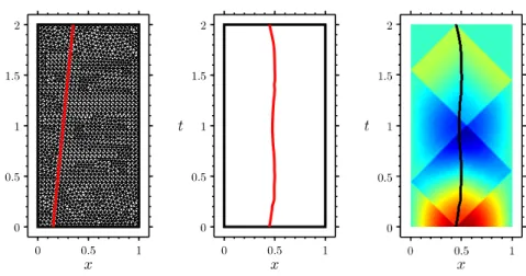
Let us consider a triangulation 𝒯ℎ of 𝑄𝑇, i.e. ∪𝐾∈𝒯ℎ𝐾 = 𝑄𝑇. We denote
ℎ := max{diam(𝐾); 𝐾 ∈ 𝒯ℎ}, where diam(𝐾) is the diameter of the triangle 𝐾.
In what follows, the space-time mesh 𝒯ℎis built from a discretization of the border
of 𝑄𝑇 and the curve 𝛾 (see Figure 5). Thus, the fineness of 𝒯ℎ will be given either
by ℎ or by the number 𝑁𝒯 of vertices per unit of length. This also means that
some vertices are supported on 𝛾, making the mesh well-adapted to the control trajectory. The mesh is generated using the software FreeFEM++ (see [17]).
The finite-dimensional space Φℎ must be chosen such that 𝐿𝜙ℎ belongs to
𝐿2(0, 𝑇 ; 𝐿2(Ω)), for any 𝜙ℎ∈ Φℎ. Therefore, any space of functions continuously
differentiable with respect to both 𝑥 and 𝑡 is a conformal approximation of Φ. We define the space Φℎ as follows
Φℎ:= {︁ 𝜙ℎ∈ 𝐶 1 (𝑄𝑇); 𝜙ℎ|𝐾∈P(𝐾), ∀𝐾 ∈ 𝒯ℎ, 𝜙ℎ= 0on Σ𝑇 }︁ ⊂ Φ, whereP(𝐾)stands for the complete Hsieh-Clough-Tocher finite element (HCT for
short) of class 𝐶1. It is a so-called composite finite element. It involves 12 degrees
of freedom which are, for each triangle 𝐾, the values of 𝜙ℎ, 𝜙ℎ,𝑥, 𝜙ℎ,𝑡on the three
vertices, and the values of the normal derivative of 𝜙 in the middle of the three edges. We refer to [12] and [5, 28] for the precise definition and the implementation of such finite element. We also introduce the finite-dimensional space
Λℎ:=
{︁
𝜆ℎ∈ 𝐶0(𝑄𝑇); 𝜆ℎ|𝐾∈Q(𝐾), ∀𝐾 ∈ 𝒯ℎ, 𝜆ℎ= 0on Σ𝑇
}︁
⊂ Λ, whereQ(𝐾)is the space of affine functions in both 𝑥 and 𝑡 on the element 𝐾.
Let 𝑛ℎ= dim(Φℎ)and 𝑚ℎ= dim(Λℎ). We define the matrices 𝐴𝑟,ℎ∈R𝑛ℎ,𝑛ℎ,
𝐵ℎ∈R𝑚ℎ,𝑛ℎ, 𝑀
ℎ∈R𝑚ℎ,𝑚ℎ and the vector 𝐿
ℎ∈R𝑛ℎ by
⟨𝐴𝑟,ℎ{𝜙ℎ}, {𝜙ℎ}⟩ = 𝑎𝑟(𝜙ℎ, 𝜙ℎ), ∀𝜙ℎ, 𝜙ℎ∈ Φℎ,
⟨𝐵ℎ{𝜙ℎ}, {𝜆ℎ}⟩ = 𝑏(𝜙ℎ, 𝜆ℎ), ∀𝜙ℎ∈ Φℎ, ∀𝜆ℎ∈ Λℎ,
⟨𝑀ℎ{𝜆ℎ}, {𝜆ℎ}⟩ = ⟨𝜆ℎ, 𝜆ℎ⟩Λ, ∀𝜆ℎ, 𝜆ℎ∈ Λℎ,
⟨𝐿ℎ, {𝜙ℎ}⟩ = ℓ(𝜙ℎ), ∀𝜙ℎ∈ Φℎ,
where {𝜙ℎ} ∈R𝑛ℎ and {𝜆ℎ} ∈R𝑚ℎ denote the vectors associated with 𝜙ℎ∈ Φℎ
and 𝜆ℎ∈ Λℎ respectively. With these notations, the discrete mixed formulation
(20) reads as follows: find {𝜙ℎ} ∈R𝑛ℎ and {𝜆ℎ} ∈R𝑚ℎ such that (︃ 𝐴𝑟,ℎ −𝐵𝑇ℎ −𝐵ℎ 0 )︃ (︃ {𝜙ℎ} {𝜆ℎ} )︃ = (︃ 𝐿ℎ 0 )︃ . (22)
For any 𝑟 > 0, the matrix 𝐴𝑟,ℎ is symmetric and positive definite. However, the
matrix in (22) is symmetric but not positive definite. The system (22) is solved by the LU method with FreeFEM++ (see [17]).
3.3 Discrete inf-sup test
Here, we test numerically the discrete inf-sup condition (21), and more precisely the property infℎ>0𝛿ℎ > 0. For simplicity, we take 𝜏 = 𝑟 > 0 in (16), so that
𝑎𝑟,ℎ(𝜙, 𝜙) = ⟨𝜙, 𝜙⟩Φfor all 𝜙, 𝜙 ∈ Φ. It is readily seen (see [10]) that the discrete
inf-sup constant satisfies 𝛿ℎ= inf {︁√ 𝜇; 𝐵ℎ𝐴−1𝑟,ℎ𝐵 𝑇 ℎ{𝜆ℎ} = 𝜇 𝑀ℎ{𝜆ℎ}, ∀{𝜆ℎ} ∈R𝑚ℎ∖ {0} }︁ . (23) For any ℎ > 0, the matrix 𝐵ℎ𝐴−1𝑟,ℎ𝐵ℎ𝑇 is symmetric and positive definite, so the
constant 𝛿ℎis strictly positive. The generalized eigenvalue problem (23) is solved
by the inverse power method (see [11]). Given {𝑢0 ℎ} ∈R
𝑚ℎ such that ‖{𝑢0
ℎ}‖2= 1,
for any 𝑛 ∈N, compute iteratively ({𝜙𝑛ℎ}, {𝜆 𝑛 ℎ}) ∈R 𝑛ℎ× R𝑚ℎ and {𝑢𝑛+1ℎ } ∈R 𝑚ℎ as follows ⎧ ⎨ ⎩ 𝐴𝑟,ℎ{𝜙𝑛ℎ} − 𝐵 𝑇 ℎ{𝜆 𝑛 ℎ} = 0, 𝐵ℎ{𝜙𝑛ℎ} = 𝑀ℎ{𝑢𝑛ℎ}, {𝑢𝑛+1ℎ } = {𝜆 𝑛 ℎ} ‖{𝜆𝑛 ℎ}‖2 .
The discrete inf-sup constant 𝛿ℎ is then given by 𝛿ℎ= lim𝑛→∞‖{𝜆𝑛ℎ}‖− 1 2 2 .
We now compute 𝛿ℎ for decreasing values of the fineness ℎ, and for different
trajectory 𝛾 defined in (Ex1–𝛾). The values that we obtain are collected in Table 1. In view of the results for 𝑟 = 10−2, the constant 𝛿
ℎdoes not seem to be uniformly
bounded by below as ℎ → 0. Thus, we may conclude that the finite elements used here do not “pass” the discrete inf-sup test. As we shall see in the next section, this fact does not prevent the convergence of the sequences (𝜙ℎ)ℎ>0and (𝜆ℎ)ℎ>0,
at least for the cases we have considered. Interestingly, we also observe that 𝛿ℎ
remains bounded by below with respect to ℎ when 𝑟 depends appropriately on ℎ, as for instance in the case 𝑟 = ℎ2.
ℎ (×10−2) 6.46 3.51 2.66 2.17 1.37 1.21 𝑟 = 10−2 1.8230 1.7947 1.7845 1.6749 1.6060 1.5008
𝑟 = ℎ 1.4575 1.3806 1.3269 1.2402 1.4188 1.3851 𝑟 = ℎ2 1.8873 1.8885 1.8783 1.8697 1.8982 1.8920
Tab. 1:Discrete inf-sup constant 𝛿ℎw.r.t. ℎ and 𝑟, for 𝛾 defined in (Ex1–𝛾).
4 Numerical simulations
In this section, we solve on various examples the discrete mixed formulation (20) to compute the HUM control for (1) and the associated controlled state. First, we determine the rate of convergence of the approximated control/controlled state, as the discretization parameter ℎ goes to zero. Second, for stationary control points 𝛾 ≡ 𝑥0, we illustrate the blow-up of the cost of control at non-strategic
points. Finally, we introduce a gradient-type algorithm to solve the problem (12) of optimizing the support of control. The algorithm is then tested on two different initial data. From now on, we set 𝑇 = 2 and 𝑟 = 10−2.
4.1 Convergence of the approximated control
In order to measure the rate of convergence of the approximated control with respect to the mesh fineness ℎ, we use the initial datum
𝑦0(𝑥) = sin(𝜋𝑥), 𝑦1(𝑥) = 0, ∀𝑥 ∈ Ω, (Ex1–y0)
and the control trajectory 𝛾(𝑡) = 1 5+ 3 5 𝑡 𝑇, ∀𝑡 ∈ [0, 𝑇 ]. (Ex1–𝛾) This curve 𝛾 is an admissible trajectory (see [8, Example 3.2]), i.e. the system (1) is controllable. To compare with the approximated solution (𝜙ℎ, 𝜆ℎ) of (20),
using the optimality condition (8), we compute another approximation (𝜙, 𝜆) by Fourier expansion (see Appendix A), with 𝑁𝐹 = 100 harmonics. We then
evaluate the errors ‖𝜙(𝛾, ·) − 𝜙ℎ(𝛾, ·)‖Hand ‖𝜆 − 𝜆ℎ‖Λfor the six levels of fineness
𝑁𝒯 = 25, 50, 75, 100, 125, 150. We gather the results in Table 2 and display them
in Figure 1. By linear regression, we find a convergence rate in ℎ0.44 for 𝜙 ℎ and
in ℎ0.48for 𝜆
ℎ. In Figure 3, we represent the adjoint state 𝜙ℎand the controlled
state 𝜆ℎ, for 𝑁𝒯 = 150. The HUM control 𝑣ℎ computed from 𝜙ℎby (9) is shown
in Figure 2, together with the “exact” control 𝑣 obtained by Fourier expansion.
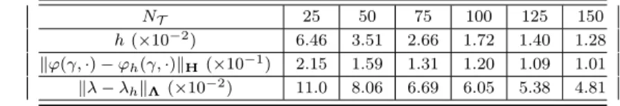
𝑁𝒯 25 50 75 100 125 150
ℎ (×10−2) 6.46 3.51 2.66 1.72 1.40 1.28 ‖𝜙(𝛾, ·) − 𝜙ℎ(𝛾, ·)‖H(×10−1) 2.15 1.59 1.31 1.20 1.09 1.01
‖𝜆 − 𝜆ℎ‖Λ(×10−2) 11.0 8.06 6.69 6.05 5.38 4.81
Tab. 2:(Ex1) – Error on the approximated solution (𝜙ℎ, 𝜆ℎ)of (20) w.r.t. ℎ.
Fig. 1:(Ex1) – Error on the approximated solution (𝜙ℎ, 𝜆ℎ)of (20) vs. ℎ –
‖𝜙(𝛾, ·) − 𝜙ℎ(𝛾, ·)‖H(•), ‖𝜆 − 𝜆ℎ‖Λ(■).
Fig. 2:(Ex1) – Controls 𝑣ℎ(–) and 𝑣 (–),
for 𝑁𝒯 = 150.
4.2 Blow-up at non-strategic points
In the case of a stationary control point 𝛾 ≡ 𝑥0∈ Ω, it is well-known that one has
to choose a so-called strategic point (see [26]) to ensure the controllability of (1). A point 𝑥0 is strategic if and only if sin(𝑝𝜋𝑥0) ̸= 0for every 𝑝 ≥ 1. Moreover, a
given initial datum (𝑦0, 𝑦1) ∈ Vcan be controlled if and only if sin(𝑝𝜋𝑥0) ̸= 0for
Fig. 3:(Ex1) – Iso-values of the adjoint state 𝜙ℎ(left) and controlled state 𝜆ℎ(right), for
𝑁𝒯 = 150.
Therefore, for (𝑦0, 𝑦1) ∈ Vfixed, we expect the cost of control to blow up as 𝑥0
gets closer to a non-strategic location. To illustrate this property, we use the initial datum
𝑦0(𝑥) = sin(2𝜋𝑥), 𝑦1(𝑥) = 0, ∀𝑥 ∈ Ω, (Ex2–y0)
and we evaluate the functional 𝐽(𝑥0)(cf. (11)) for several control locations 𝑥0spread
in the interval (1 4,
1
2). With the initial datum considered, 𝑥 ⋆
= 12 is the unique non-strategic point. In Figure 4, we display 𝐽(𝑥0)w.r.t. the distance |𝑥⋆− 𝑥0|. As
expected, we note that the cost of control blows up when 𝑥0→ 𝑥⋆. More precisely,
we have 𝐽(𝑥0) ∼𝑥⋆𝐶0|𝑥⋆− 𝑥0|−1.97.
4.3 Optimization of the support using splines
We now focus on solving numerically the problem (12) with a gradient-type algo-rithm. To do so, the control trajectories 𝛾 considered are degree 5 splines adapted to a fixed subdivision of [0, 𝑇 ]. For any integer 𝑁 ≥ 1, we denote 𝑆𝑁= (𝑡𝑖)0≤𝑖≤𝑁
the regular subdivision of [0, 𝑇 ] in 𝑁 intervals. With 𝜅 = 𝑇/𝑁, the subdivision points are 𝑡𝑖= 𝑖 𝜅. In the simulations below, we use 𝑁 = 20. We then define the
set 𝒮5of degree 5 splines adapted to the subdivision 𝑆𝑁. Such a spline 𝛾 ∈ 𝒮5is
of class 𝐶2
([0, 𝑇 ])and is uniquely determined by the 3(𝑁 + 1) conditions 𝛾(𝑡𝑖) = 𝑥𝑖, 𝛾′(𝑡𝑖) = 𝑝𝑖, 𝛾′′(𝑡𝑖) = 𝑐𝑖, 0 ≤ 𝑖 ≤ 𝑁,
Fig. 4:(Ex2) – 𝐽(𝑥0)vs. |𝑥⋆− 𝑥0|, for stationary control points 𝑥0.
where x = (𝑥𝑖)0≤𝑖≤𝑁, p = (𝑝𝑖)0≤𝑖≤𝑁 and c = (𝑐𝑖)0≤𝑖≤𝑁 represent the spline
parameters. We also introduce the degree 5 polynomial basis (𝑃𝑘,𝑙)𝑘=0,1,2 𝑙=0,1 on [0, 1] characterized by 𝑃(𝑘 ′) 𝑘,𝑙 (𝑙 ′ ) = 𝛿𝑘,𝑘′𝛿𝑙,𝑙′, for 𝑘, 𝑘′∈ {0, 1, 2}, 𝑙, 𝑙′∈ {0, 1}. Here, 𝑃(𝑘′)
𝑘,𝑙 stands for the 𝑘
′-th derivative of 𝑃
𝑘,𝑙 and 𝛿𝑘,𝑘′ is the Kronecker delta,
i.e. 𝛿𝑘,𝑘′ = 1if 𝑘 = 𝑘′ and 𝛿𝑘,𝑘′ = 0 otherwise. For the sake of presentation, we
briefly rename the parameters (x, p, c) = (s0
, s1, s2). It allows to decompose 𝛾 into
𝛾(𝑡) = 𝑁 ∑︁ 𝑖=1 2 ∑︁ 𝑘=0 (︁ s𝑘𝑖−1𝑃𝑘,0𝑖 (𝑡) + s 𝑘 𝑖𝑃𝑘,1𝑖 (𝑡) )︁ 1[𝑡𝑖−1,𝑡𝑖](𝑡), ∀𝑡 ∈ [0, 𝑇 ],
where we have set 𝑃𝑖
𝑘,𝑙(𝑡) = 𝜅𝑘𝑃𝑘,𝑙
(︁𝑡−𝑡
𝑖−1 𝜅
)︁
. With this decomposition, the opti-mization problem (12) is reduced to a finite-dimensional problem in the space of parameters, i.e. min 𝛾∈𝒮5 𝐽𝜀,𝜂(𝛾) = min s 𝐽̃︀𝜀,𝜂(s), where s = (x, p, c) ∈R 3(𝑁 +1) .
In order to get a descent direction for 𝐽𝜀,𝜂 at 𝛾 ∈ 𝒮5, we consider the following
variational problem: find 𝑗𝛾 ∈ 𝒮5 solution of
⟨𝑗𝛾, 𝛾⟩H+ 𝜀⟨𝑗𝛾′′, 𝛾′′⟩𝐿2(0,𝑇 )=d𝐽(𝛾; 𝛾) + 𝜀⟨𝛾′′, 𝛾′′⟩𝐿2(0,𝑇 )
+ 𝜂(𝐿(𝛾) − 𝐿)+d𝐿(𝛾; 𝛾), ∀𝛾 ∈ 𝒮5.
(24)
Indeed, using Lemma 3, we can see that d𝐽𝜀,𝜂(𝛾; 𝑗𝛾) = ‖𝑗𝛾‖2H+ 𝜀‖𝑗𝛾′′‖2𝐿2(0,𝑇 )≥ 0.
The problem (24) is solved by the finite element method using FreeFEM++. We denote by 𝑃Ωthe projection in Ω. Then, the gradient algorithm for solving (12) is
given by Algorithm 1. We point out that a re-meshing of 𝑄𝑇 is performed at each
iteration, in order to be conform with the current trajectory 𝛾𝑛. We illustrate the
algorithm on two examples.
Algo. 1:Gradient descent
InitializationChoose a trajectory 𝛾0∈ 𝒮5such that 0 < 𝛾0< 1.
For each 𝑛 ≥ 0 do
◁Compute the solution 𝜙ℎ of (20) associated with 𝛾𝑛.
◁Evaluate the costs 𝐽(𝛾𝑛)and 𝐽𝜀,𝜂(𝛾𝑛).
◁Compute the solution 𝑗𝛾𝑛 of (24).
◁Update the trajectory 𝛾𝑛 by setting
𝛾𝑛+1= 𝑃Ω(𝛾𝑛− 𝜌 𝑗𝛾𝑛), with 𝜌 > 0 fixed.
End
Example 1 – Sine function
To test Algorithm 1, we first use the initial datum
𝑦0(𝑥) = 10 sin(𝜋𝑥), 𝑦1(𝑥) = 0, ∀𝑥 ∈ Ω. (Ex3–y0)
We initialize the algorithm with the trajectory 𝛾0∈ 𝒮5 associated with the
param-eters 𝑥𝑖= 3 20+ 1 5 𝑡𝑖 𝑇, 𝑝𝑖= 1 5𝑇, 𝑐𝑖= 0, 0 ≤ 𝑖 ≤ 𝑁. (Ex3–𝛾0) We set 𝜀 = 10−4, 𝜂 = 103
, 𝐿 = 2.01 and 𝜌 = 10−2. The initial trajectory 𝛾 0, the
optimal trajectory 𝛾⋆and the optimal controlled state 𝜆⋆are displayed in Figure 5.
We observe that the optimal trajectory we get is close to a stationary control point located in 𝑥0=12, the maximum point of sin(𝜋𝑥). This is coherent with the case
of controls distributed over domains 𝑞 ⊂ 𝑄𝑇 (see [6, Example EX1]).
Example 2 – Travelling wave
To test again the similarities between the pointwise control case and the distributed control case, we now use the initial datum
Fig. 5:(Ex3) – Initial trajectory 𝛾0, optimal trajectory 𝛾⋆and optimal controlled state 𝜆⋆
(from left to right). The left figure also illustrates the type of mesh used to solve (20).
To see whether the control trajectory is likely to “follow” the wave associated with (Ex4–y0) as it is the case in [6, Example EX2]), we define the trajectories
𝑔𝑥0(𝑡) = 𝑓𝑥0(𝑡) + 0.15 cos(5𝜋(𝑡 − 𝑥0)), for any 𝑥0∈ Ω.
Here, 𝑓𝑥0 is the characteristic line “𝑥+𝑡 = 𝑥0” of the wave equation. The trajectory
𝑔1
2 is displayed in Figure 8-left. Then, for several values of 𝑥0in Ω, we evaluate
the functional 𝐽(𝑔𝑥0) associated with the initial datum (Ex4–y0). The results are
displayed in Figure 6, and we can see that 𝐽 reaches its minimum for 𝑥0= 12.
We then employ Algorithm 1 for two different initial trajectories 𝛾0 ∈ 𝒮5, respectively defined by 𝑥𝑖= 𝑔1 2(𝑡𝑖), 𝑝𝑖= 𝑔 ′ 1 2(𝑡𝑖), 𝑐𝑖= 𝑔 ′′ 1 2(𝑡𝑖), 0 ≤ 𝑖 ≤ 𝑁, (Ex4.1–𝛾0) 𝑥𝑖= 1 4+ 1 2 𝑡𝑖 𝑇, 𝑝𝑖= 1 2𝑇, 𝑐𝑖= 0, 0 ≤ 𝑖 ≤ 𝑁. (Ex4.2–𝛾0) We set 𝜀 = 10−4, 𝜂 = 103, 𝐿 = 4 and 𝜌 = 10−2. For the two examples (Ex4.1)
and (Ex4.2), we display the initial trajectory 𝛾0, the optimal trajectory 𝛾⋆ and
the optimal controlled state 𝜆⋆ in Figures 8-9 respectively. In the first setup, we
observe that the optimal trajectory remains close to the wave support, which is coherent with the distributed control case. In the second setup, the optimal trajectory also seems to get closer to the wave support, but the convergence is very slow. This can be seen in Figure 7, where the evolution of the functional 𝐽(𝛾𝑛)and
the curve length 𝐿(𝛾𝑛)are shown. The optimal costs are respectively 𝐽(𝛾⋆) = 3.92
for (Ex4.1) and 𝐽(𝛾⋆
) = 3.69for (Ex4.2). The difference is negligible compared to the initial cost 𝐽(𝛾0) = 37.45for the example (Ex4.2).
Fig. 7:(Ex4.2) – Functional 𝐽(𝛾𝑛)(left) and curve length 𝐿(𝛾𝑛)(right).
5 Conclusion
On the basis of [9] that deals with controls distributed over non-cylindrical domains, we have built a mixed formulation characterizing the HUM control acting on a moving point. The formulation involves the adjoint state and a Lagrange multiplier which turns out to coincide with the controlled state. This approach leads to a variational formulation over a Hilbert space without distinction between the space
Fig. 8:(Ex4.1) – Initial trajectory 𝛾0, optimal trajectory 𝛾⋆and optimal controlled state 𝜆⋆
(from left to right).
and time variables, making it very appropriate to our moving point situation. We have shown the well-posedness of the formulation using the observability inequality proved in [8]. At a practical level, the mixed formulation is discretized and solved in the finite element framework. The resolution amounts to solve a sparse symmetric system. From a numerical point of view, we have provided evidence of the convergence of the approximated control for regular initial data.
Still from a numerical perspective, for a fixed initial datum, we have considered the natural problem of optimizing the support of control. We have solved this problem with a simple gradient algorithm. For simplicity, the optimization is made over very regular trajectories. The results we get are similar with those obtained in [6], where the same problem is studied for controls distributed over non-cylindrical domains. Although, the convergence towards the optimal trajectory seems to be generally much slower.
This work may be extended to several directions. First, as it is done in [30] for distributed controls, one could try to justify rigorously the well-posedness of the support optimization problem. In that context, it could be interesting to find the minimal regularity necessary for the control trajectories. Besides, one could try to implement other types of algorithm for solving the problem, as for instance an algorithm based on the level-set method. Another challenge is the extension of the observability inequality to the multidimensional case, where we cannot make use of the d’Alembert formula.
Fig. 9:(Ex4.2) – Initial trajectory 𝛾0, optimal trajectory 𝛾⋆and optimal controlled state 𝜆⋆
(from left to right).
A Fourier expansion of the HUM control
In this appendix, we expand in terms of Fourier series the adjoint state 𝜙 linked to the HUM control 𝑣 by the relation (9), as well as the associated controlled state 𝑦. These expansions are used to evaluate the errors ‖𝑣 − 𝑣ℎ‖H′ and ‖𝑦 − 𝑦ℎ‖Λ in
Section 4. One can show that 𝜙 and 𝑦 take the form 𝜙(𝑥, 𝑡) =∑︁ 𝑝≥1 (︂ 𝑎𝑝cos(𝑝𝜋𝑡) + 𝑏𝑝 𝑝𝜋sin(𝑝𝜋𝑡) )︂ sin(𝑝𝜋𝑥), (25) 𝑦(𝑥, 𝑡) =∑︁ 𝑝≥1 𝑐𝑝(𝑡) sin(𝑝𝜋𝑥). (26) We set ⎧ ⎨ ⎩ 𝜉𝑝𝑎(𝑡) = cos(𝑝𝜋𝑡) sin(𝑝𝜋𝛾(𝑡)), 𝜉𝑝𝑏(𝑡) = 1 𝑝𝜋sin(𝑝𝜋𝑡) sin(𝑝𝜋𝛾(𝑡)), ∀𝑝 ≥ 1.
Injecting (25) in the terms appearing in the optimality condition (8), we get
𝑇 ∫︁ 0 𝜙(𝛾(𝑡), 𝑡)𝜙(𝛾(𝑡), 𝑡)d𝑡 = ∑︁ 𝑝,𝑞≥1 𝑎𝑝𝑎𝑞 𝑇 ∫︁ 0 𝜉𝑝𝑎𝜉𝑞𝑎+ ∑︁ 𝑝,𝑞≥1 𝑏𝑝𝑏𝑞 𝑇 ∫︁ 0 𝜉𝑝𝑏𝜉𝑞𝑏 + ∑︁ 𝑝,𝑞≥1 𝑎𝑝𝑏𝑞 𝑇 ∫︁ 0 𝜉𝑝𝑎𝜉𝑞𝑏+ ∑︁ 𝑝,𝑞≥1 𝑏𝑝𝑎𝑞 𝑇 ∫︁ 0 𝜉𝑏𝑝𝜉𝑎𝑞, (27)
𝑇 ∫︁ 0 d d𝑡𝜙(𝛾(𝑡), 𝑡)d𝑡d𝜙(𝛾(𝑡), 𝑡)d𝑡 = ∑︁ 𝑝,𝑞≥1 𝑎𝑝𝑎𝑞 𝑇 ∫︁ 0 𝜉𝑝𝑎 ′𝜉𝑞𝑎 ′+ ∑︁ 𝑝,𝑞≥1 𝑏𝑝𝑏𝑞 𝑇 ∫︁ 0 𝜉𝑝𝑏 ′𝜉𝑏 ′𝑞 + ∑︁ 𝑝,𝑞≥1 𝑎𝑝𝑏𝑞 𝑇 ∫︁ 0 𝜉𝑝𝑎 ′𝜉𝑞𝑏 ′+ ∑︁ 𝑝,𝑞≥1 𝑏𝑝𝑎𝑞 𝑇 ∫︁ 0 𝜉𝑏 ′𝑝 𝜉𝑎 ′𝑞 , (28) ∫︁ Ω 𝑦0𝜙1= 1 2 ∑︁ 𝑝≥1 𝑐𝑝(𝑦0)𝑏𝑝 and ⟨𝑦1, 𝜙0⟩−1,1= 1 2 ∑︁ 𝑝≥1 𝑐𝑝(𝑦1)𝑎𝑝. (29)
Here, 𝑐𝑝(𝑦0)and 𝑐𝑝(𝑦1)are the Fourier coefficients of 𝑦0and 𝑦1. Thus, optimality
condition (8) can be rewritten
⟨ ℳ𝛾 (︃ {𝑎𝑝}𝑝≥1 {𝑏𝑝}𝑝≥1 )︃ , (︃ {𝑎𝑞}𝑞≥1 {𝑏𝑞}𝑞≥1 )︃⟩ = ⟨ ℱy0, (︃ {𝑎𝑞}𝑞≥1 {𝑏𝑞}𝑞≥1 )︃⟩ , ∀(𝑎𝑞, 𝑏𝑞)𝑞≥1, (30) where the positive definite matrix ℳ𝛾 and the vector ℱy0 are obtained from
(27-28) and (29) respectively. The resolution of the infinite-dimensional system (30) (reduced to a finite-dimensional one by truncation) provides an approximation of the adjoint state 𝜙 linked to the HUM control 𝑣 by (9).
Injecting (26) in the wave equation (1), we find that 𝑐𝑝(𝑡)satisfies
{︃ 𝑐′′𝑝(𝑡) + (𝑝𝜋)2𝑐𝑝(𝑡) = 2𝑣(𝑡) sin(𝑝𝜋𝛾(𝑡)), ∀𝑡 > 0, 𝑐𝑝(0) = 𝑐𝑝(𝑦0), 𝑐′𝑝(0) = 𝑐𝑝(𝑦1). We then have 𝑐𝑝(𝑡) = 𝑐𝑝(𝑦0) cos(𝑝𝜋𝑡) + 𝑐𝑝(𝑦1) 𝑝𝜋 sin(𝑝𝜋𝑡) + 2 𝑝𝜋 𝑡 ∫︁ 0 𝑣(𝑠) sin(𝑝𝜋𝛾(𝑠)) sin(𝑝𝜋(𝑡 − 𝑠))d𝑠.
Finally, by integration by parts, we deduce
𝑐𝑝(𝑡) = 𝑐𝑝(𝑦0) cos(𝑝𝜋𝑡) + 𝑐𝑝(𝑦1) 𝑝𝜋 sin(𝑝𝜋𝑡) + 2 𝑝𝜋 𝑡 ∫︁ 0 𝜙(𝛾(𝑠), 𝑠) sin(𝑝𝜋𝛾(𝑠)) sin(𝑝𝜋(𝑡 − 𝑠))d𝑠 − 2 𝑡 ∫︁ 0 d d𝑠𝜙(𝛾(𝑠), 𝑠) sin(𝑝𝜋𝛾(𝑠)) cos(𝑝𝜋(𝑡 − 𝑠))d𝑠 + 2 𝑡 ∫︁ 0 d d𝑠𝜙(𝛾(𝑠), 𝑠) cos(𝑝𝜋𝛾(𝑠))𝛾 ′ (𝑠) sin(𝑝𝜋(𝑡 − 𝑠))d𝑠.
References
[1] A. Agresti, D. Andreucci, and P. Loreti. Observability for the wave equation with variable support in the Dirichlet and Neumann cases. In International Conference on Informatics in Control, Automation and Robotics, pages 51–75.
Springer, 2018.
[2] A. Bamberger, J. Jaffre, and J.-P. Yvon. Punctual control of a vibrating string: numerical analysis. Comput. Math. Appl., 4(2):113–138, 1978.
[3] C. Bardos, G. Lebeau, and J. Rauch. Sharp sufficient conditions for the observation, control, and stabilization of waves from the boundary. SIAM J. Control Optim., 30(5):1024–1065, 1992.
[4] M. Berggren and R. Glowinski. Controllability issues for flow-related models: a computational approach. Technical report, 1994.
[5] M. Bernadou and K. Hassan. Basis functions for general Hsieh-Clough-Tocher triangles, complete or reduced. Internat. J. Numer. Methods Engrg., 17(5):784– 789, 1981.
[6] A. Bottois, N. Cîndea, and A. Münch. Optimization of non-cylindrical domains for the exact null controllability of the 1D wave equation. To be published, 2019.
[7] F. Brezzi and M. Fortin. Mixed and hybrid finite element methods, volume 15 of Springer Series in Computational Mathematics. Springer-Verlag, New York, 1991.
[8] C. Castro. Exact controllability of the 1-D wave equation from a moving interior point. ESAIM Control Optim. Calc. Var., 19(1):301–316, 2013. [9] C. Castro, N. Cîndea, and A. Münch. Controllability of the linear
one-dimensional wave equation with inner moving forces. SIAM J. Control Optim., 52(6):4027–4056, 2014.
[10] D. Chapelle and K.-J. Bathe. The inf-sup test. Comput. & Structures, 47(4-5):537–545, 1993.
[11] F. Chatelin. Eigenvalues of matrices, volume 71 of Classics in Applied Mathe-matics. Society for Industrial and Applied Mathematics (SIAM), Philadelphia, PA, 2012. With exercises by Mario Ahués and the author, Translated with additional material by Walter Ledermann, Revised reprint of the 1993 edition [ MR1232655].
[12] P. Ciarlet. The finite element method for elliptic problems, volume 40 of Clas-sics in Applied Mathematics. Society for Industrial and Applied Mathematics (SIAM), Philadelphia, PA, 2002. Reprint of the 1978 original [North-Holland, Amsterdam; MR0520174 (58 #25001)].
[13] N. Cîndea and A. Münch. A mixed formulation for the direct approximation of the control of minimal 𝐿2-norm for linear type wave equations. Calcolo,
52(3):245–288, 2015.
[14] R. Dáger and E. Zuazua. Wave propagation, observation and control in 1-𝑑 flexible multi-structures, volume 50 of Mathématiques & Applications (Berlin) [Mathematics & Applications]. Springer-Verlag, Berlin, 2006.
[15] S. Ervedoza and E. Zuazua. A systematic method for building smooth controls for smooth data. Discrete Contin. Dyn. Syst. Ser. B, 14(4):1375–1401, 2010. [16] R. Glowinski, J.-L. Lions, and J. He. Exact and approximate controllability for distributed parameter systems, volume 117 of Encyclopedia of Mathematics and its Applications. Cambridge University Press, Cambridge, 2008. A numerical approach.
[17] F. Hecht. New development in freefem++. J. Numer. Math., 20(3-4):251–265, 2012.
[18] A. Henrot, W. Horn, and J. Sokołowski. Domain optimization problem for stationary heat equation. Appl. Math. Comput. Sci., 6(2):353–374, 1996. Shape optimization and scientific computations (Warsaw, 1994).
[19] A. Henrot and J. Sokołowski. A shape optimization problem for the heat equation. In Optimal control (Gainesville, FL, 1997), volume 15 of Appl. Optim., pages 204–223. Kluwer Acad. Publ., Dordrecht, 1998.
[20] A. Khapalov. Controllability of the wave equation with moving point control. Appl. Math. Optim., 31(2):155–175, 1995.
[21] A. Khapalov. Mobile point controls versus locally distributed ones for the controllability of the semilinear parabolic equation. SIAM J. Control Optim., 40(1):231–252, 2001.
[22] A. Khapalov. Observability and stabilization of the vibrating string equipped with bouncing point sensors and actuators. Math. Methods Appl. Sci., 24(14):1055–1072, 2001.
[23] J. Le Rousseau, G. Lebeau, P. Terpolilli, and E. Trélat. Geometric control condition for the wave equation with a time-dependent observation domain. Anal. PDE, 10(4):983–1015, 2017.
[24] J.-L. Lions. Some methods in the mathematical analysis of systems and their control. Kexue Chubanshe (Science Press), Beijing; Gordon & Breach Science Publishers, New York, 1981.
[25] J.-L. Lions. Contrôlabilité exacte, perturbations et stabilisation de systèmes distribués. Tome 1, volume 8 of Recherches en Mathématiques Appliquées [Research in Applied Mathematics]. Masson, Paris, 1988. Contrôlabilité exacte. [Exact controllability], With appendices by E. Zuazua, C. Bardos, G. Lebeau and J. Rauch.
[26] J.-L. Lions. Pointwise control for distributed systems. In Control and estima-tion in distributed parameter systems, pages 1–39. SIAM, 1992.
[27] J.-L. Lions and E. Magenes. Non-homogeneous boundary value problems and applications. Vol. I. Springer-Verlag, New York-Heidelberg, 1972. Trans-lated from the French by P. Kenneth, Die Grundlehren der mathematischen Wissenschaften, Band 181.
[28] A. Meyer. A simplified calculation of reduced HCT-basis functions in a finite element context. Comput. Methods Appl. Math., 12(4):486–499, 2012. [29] A. Münch. A uniformly controllable and implicit scheme for the 1-D wave
equation. M2AN Math. Model. Numer. Anal., 39(2):377–418, 2005.
[30] F. Periago. Optimal shape and position of the support for the internal exact control of a string. Systems Control Lett., 58(2):136–140, 2009.
[31] Á. M. Ramos, R. Glowinski, and J. Périaux. Pointwise control of the Burgers equation and related Nash equilibrium problems: computational approach. J. Optim. Theory Appl., 112(3):499–516, 2002.