HAL Id: tel-01401552
https://tel.archives-ouvertes.fr/tel-01401552v2
Submitted on 14 Mar 2017HAL is a multi-disciplinary open access
archive for the deposit and dissemination of sci-entific research documents, whether they are pub-lished or not. The documents may come from teaching and research institutions in France or abroad, or from public or private research centers.
L’archive ouverte pluridisciplinaire HAL, est destinée au dépôt et à la diffusion de documents scientifiques de niveau recherche, publiés ou non, émanant des établissements d’enseignement et de recherche français ou étrangers, des laboratoires publics ou privés.
pollution sources
Louis Marelle
To cite this version:
Louis Marelle. Regional modeling of aerosols and ozone in the arctic : air quality and radiative impacts from local and remote pollution sources. Ocean, Atmosphere. Université Pierre et Marie Curie - Paris VI, 2016. English. �NNT : 2016PA066190�. �tel-01401552v2�
DES SCIENCES DE L’ENVIRONNEMENT D’ILE DE FRANCE
T H È S E
pour obtenir le grade de
Docteur en Sciences
de l’Université Pierre et Marie Curie
Spécialité : Physique de l’atmosphère
Présentée et soutenue par
Louis Marelle
Modélisation régionale des polluants à courte
durée de vie (aérosols, ozone) en Arctique
Thèse dirigée par Kathy S. Law
préparée au Laboratoire ATmosphère, Milieux, Observations Spatiales financée par TOTAL S.A. (convention CIFRE N∘2012/0999)
Jury :
Président : François Ravetta
Rapporteurs : Terje K. Berntsen Karine Sartelet
Examinateur : Alfons Schwarzenboeck
Directrice : Kathy S. Law
Co-Directeur : Jean-Christophe Raut
Invités : Jennie L. Thomas
La région arctique s’ouvre peu à peu aux activités humaines, en raison du réchauffement climatique et de la fonte des glaces, dûs en partie à l’effet de polluants à courte durée de vie (aérosols, ozone). Dans le futur, les émissions de ces polluants liées à la navigation et à l’extraction de ressources en Arctique pourraient augmenter, et devenir prépondérantes comparées à la source historique liée au transport de pollution depuis les moyennes latitudes. Dans cette thèse, j’effectue des simulations régionales de la troposphère arctique avec le modèle WRF-Chem, combiné à de nouveaux inventaires des émissions de pollution locales en Arctique (navigation et torches pétrolières). Deux cas d’étude issus de campagnes de mesure par avion sont analysés. Premièrement, j’étudie un évènement de transport d’aérosols depuis l’Europe au printemps 2008, afin d’améliorer les connaissances sur cette source majeure de pollution Arctique. Deuxièmement, je détermine l’impact des émissions de la navigation en Norvège en été 2012, où la navigation Arctique est actuellement la plus intense. J’utilise ces cas d’étude pour valider la pollution modélisée et améliorer WRF-Chem en Arctique. J’effectue avec ce modèle amélioré des simulations des impacts actuels (2012) et futurs (2050) de la navigation et des torches pétrolières en Arctique sur la qualité de l’air et le bilan radiatif. Les résultats indiquent que les torches sont et devraient rester une source majeure d’aérosols de carbone suie réchauffants en Arctique. La navigation est une source de pollution importante en été ; et en 2050, la navigation de diversion à travers l’Arctique pourrait devenir une source majeure de pollution locale.
The Arctic is increasingly open to human activity due to rapid warming, associated with decreased sea ice extent. This warming is due, in part, to the effect of short-lived atmo-spheric pollutants (aerosols, ozone). Emissions from oil and gas extraction and marine traffic should increase in the future, and their impacts might become significant compared to the now predominant source due to pollution transport from the mid-latitudes. In this thesis, regional simulations of the Arctic troposphere are performed with the WRF-Chem model, combined with new emission estimates for oil and gas extraction and shipping in the Arctic. The model is used to analyze two case studies from recent airborne measurement datasets: POLARCAT-France in 2008, ACCESS in 2012. First, I investigate an aerosol transport event from Europe to the Arctic in spring 2008, in order to improve our understanding of this major source of Arctic pollution. Second, I determine the air quality and radiative impacts of shipping emissions in Northern Norway in summer 2012, where most current Arctic shipping occurs. I use these results to validate modeled pollution, and to improve WRF-Chem for Arctic studies. The updated model is used to investigate the current (2012) and future (2050) impacts of Arctic shipping and Arctic gas flaring in terms of air quality and radiative effects. Results show that Arctic flaring emissions are and should remain a major source of local black carbon aerosols, causing warming, and that Arctic shipping is already a strong source of aerosols and ozone during summer. In 2050, diversion shipping through the Arctic Ocean could become one of the main sources of local surface aerosol and ozone pollution.
Je souhaiterais tout d’abord remercier Kathy Law et Jean-Christophe Raut, pour avoir accepté de diriger cette thèse. Merci de m’avoir accompagné et guidé pendant ces quatre années, du stage à la soutenance, tout en me laissant la liberté dont j’avais besoin. J’ai apprécié vos conseils toujours justes, votre disponibilité, votre soutien. Cette thèse n’aurait pas non plus été possible sans le financement de Total, et je voudrais ici remercier ceux qui se sont démenés pour la mettre en place, en particulier Philippe Ricoux et Olivier Duclaux, mais aussi tous ceux qui se sont intéressés à mon travail. Je remercie enfin mon jury de thèse, mon comité de thèse, et tous ceux qui ont contribué à améliorer ce travail.
Cette thèse n’aurait pas été ce qu’elle est sans Jennie Thomas, ma co-directrice de thèse officieuse. Jennie, you had more success in helping me write papers than in convincing me to appreciate quinoa and kale, but don’t give up, maybe some day I will.
Je remercie également le LATMOS, et l’équipe Tropo, où j’ai été chaleureusement ac-cueilli pendant cette thèse, et tous ceux qui ont rendu ces années au LATMOS agréables, trop nombreux pour tous les nommer ici. Des remerciements particuliers à Ludivine pour sa bonne humeur, à Aurélien pour sa mauvaise humeur, et merci à tous les deux pour le café du commerce/groupe de soutien/café-philo du 3ème étage qui est très vite devenu une
habitude et une nécessité. Merci aussi à tous les occupants du bureau 316 où je me suis tout de suite senti chez moi: Jaime, Katerina, Christophe, Thierno, Tommaso, Xiaoxa.
Après le travail, j’ai pu compter sur le soutien d’Hugues, Arnaud, Rodérick, Elsa, et de bien d’autres qui, au détour d’un verre ou d’un dîner, ont parfois dû m’écouter soliloquer au sujet des paramétrisations de cumulus ou des modules de photochimie. Je remercie aussi les musiciens avec qui j’ai produit un bruit innommable tous les dimanches matin.
Merci au delà des mots à Leïla, qui a dû me supporter plus que tous les autres, et à qui je rappelle ici pour la millième fois que je n’ai pas écrit une thèse sur «les ours polaires».
Et, ici en dernier mais avant tout, merci à Maman, Lucie, Julien et Arnaud, présents dans les bons moments comme dans les plus difficiles.
Introduction en français 15
Introduction 19
1 Climate change and air pollution in the Arctic 23
1.1 Global air pollution and climate change . . . 23
1.1.1 Air pollution . . . 23
1.1.2 Global climate change . . . 25
1.2 Arctic climate change: causes and future projections . . . 30
1.2.1 What is the Arctic? . . . 30
1.2.2 Current Arctic warming . . . 31
1.2.3 Causes of Arctic warming . . . 32
1.2.4 Future projections . . . 32
1.3 Arctic air pollution . . . 33
1.3.1 Arctic Haze . . . 33
1.3.2 Arctic air pollution transported from the mid-latitudes . . . 33
1.3.3 Developing local sources of Arctic pollution . . . 36
1.4 Scientific challenges in modeling Arctic aerosols and ozone and their impacts . 38 1.4.1 Modeling aerosol and ozone pollution from long-range transport . . . . 39
1.4.2 Modeling aerosol and ozone pollution from local Arctic sources . . . . 39
2 Tropospheric ozone and tropospheric aerosols in the Arctic 41 2.1 Tropospheric ozone . . . 41
2.1.1 Introduction: stratospheric and tropospheric ozone . . . 41
2.1.2 Chemical O3 production in the troposphere from NOxand VOC . . . 42
2.1.3 Photochemical sinks of ozone, HOx and NOx in the troposphere . . . . 44
2.1.4 Dry deposition of NOx and O3 . . . 45
2.1.5 Peroxyacetyl nitrate (PAN) as a NOx reservoir in the troposphere . . . 45
2.1.6 The global budget of tropospheric ozone . . . 46
2.1.7 Radiative effects of tropospheric ozone . . . 47
2.1.8 Tropospheric ozone in the Arctic . . . 48
2.2 Tropospheric aerosols . . . 50
2.2.1 Global aerosol sources . . . 50
2.2.2 Aerosol properties: chemical composition, mixing state, size . . . 50
2.2.3 Aerosol processes: from nucleation to removal . . . 54
2.2.4 Aerosol optical properties . . . 57
2.2.5 Aerosol radiative effects . . . 60
3 Methods: modeling tools, emission inventories and Arctic measurements 65 3.1 Modeling the air quality and radiative impacts of short-lived pollutants in the Arctic. . . 65
3.1.1 Regional meteorology-chemistry-aerosol modeling with WRF-Chem . . 66
3.1.2 Lagrangian modeling with FLEXPART-WRF . . . 70
3.2 Air pollutant emissions from global and local Arctic pollution sources . . . 71
3.2.1 Global anthropogenic emissions from ECLIPSEv5 and HTAPv2 . . . . 71
3.2.2 Biomass burning emissions . . . 76
3.2.3 Natural emisssions calculated online within WRF-Chem . . . 77
3.2.4 Local Arctic pollutant emissions from oil and gas extraction . . . 77
3.2.5 Local Arctic emissions from shipping . . . 79
3.3 Aerosol and ozone measurements in the Arctic . . . 84
3.3.1 Surface measurements . . . 85
3.3.2 POLARCAT-France and ACCESS aircraft measurement campaigns in the Arctic . . . 85
4 Transport of pollution from the mid-latitudes to the Arctic during POLARCAT-France 87 4.1 Motivation . . . 87
4.2 Transport of anthropogenic and biomass burning aerosols from Europe to the Arctic during spring 2008 (Marelle et al., 2015). . . 89
4.2.1 Abstract . . . 89
4.2.2 Introduction . . . 89
4.2.3 Methods . . . 91
4.2.4 Meteorological context during the spring POLARCAT-France campaign 96 4.2.5 Model validation . . . 97
4.2.6 The origin and properties of springtime aerosols during POLARCAT-France . . . 100
4.2.7 Impacts of European aerosol transport on the Arctic . . . 109
4.2.8 Summary and conclusions . . . 112
4.3.1 Aerosol transport to the Arctic . . . 115
4.3.2 Ozone transport to the Arctic in these simulations, and in the related work of Thomas et al. (2013) . . . 116
5 Current impacts of Arctic shipping in Northern Norway 117 5.1 Motivation . . . 117
5.2 Air quality and radiative impacts of Arctic shipping emissions in the sum-mertime in northern Norway: from the local to the regional scale (Marelle et al., 2016). . . 119
5.2.1 Abstract . . . 119
5.2.2 Introduction . . . 119
5.2.3 The ACCESS aircraft campaign . . . 121
5.2.4 Modeling tools . . . 123
5.2.5 Ship emission evaluation . . . 128
5.2.6 Modeling the impacts of ship emissions along the Norwegian coast . . 134
5.2.7 Conclusions . . . 143
5.3 Main insights from the study . . . 145
6 Current and future impacts of local Arctic sources of aerosols and ozone 147 6.1 Introduction and motivation . . . 147
6.2 Methods . . . 148
6.3 Model updates for quasi-hemispheric Arctic simulations . . . 151
6.4 Model validation . . . 154
6.5 Model internal variability and noise: issues when quantifying sensitivities to small emission perturbations with WRF-Chem . . . 158
6.6 Local and distant contributions to surface concentrations and BC deposition in the Arctic . . . 160
6.6.1 Surface concentrations and BC deposition in spring and summer 2012 160 6.6.2 Surface concentrations and BC deposition in spring and summer 2050 (2050 emissions) . . . 164
6.7 Vertical distribution of Arctic aerosol and ozone pollution from remote and local sources . . . 167
6.8 Radiative effects of aerosols and ozone in the Arctic. . . 169
6.8.1 Direct radiative effects of pollution aerosols and ozone in the Arctic. . 169
6.8.2 Semi-direct and indirect radiative effects. . . 172
6.9 Conclusions and perspectives . . . 174
General Conclusions 177
L’Arctique est la région du monde qui se réchauffe le plus rapidement ; les températures de surface y augmented plus de deux fois plus vite que la moyenne globale (IPCC, 2013b). Ce réchauffement est dû principalement à l’effet des gaz à effet de serre « bien mélangés », comme le CO2 et le méthane, mais aussi à l’effet d’espèces à plus courtes durées de vie :
les aérosols et l’ozone (Shindell et al., 2006). Les émissions locales de pollution en Arctique sont supposées faibles. Pour cette raison, des études précédentes indiquent que la source principale de pollution à l’ozone et aux aérosols en Arctique au 20ème siècle est le transport
de polluants depuis les moyennes latitudes (Barrie, 1986), tandis que la cause principale du réchauffement Arctique est le réchauffement des moyennes latitudes suivi du transport de chaleur vers l’Arctique (Shindell, 2007).
Le réchauffement de l’Arctique et la fonte des glaces qui lui est associée (IPCC, Kirtman et al., 2013) pourraient progressivement permettre le développement industriel de cette région, en particulier des activités liées au traffic maritime et à l’extraction de ressources. Ceci pourrait entraîner une croissance importante des émissions locales de polluants à courte durée de vie et de leurs précurseurs en Arctique (IPCC, 2014), alors que dans le reste de la planète ces émissions devraient diminuer (IPCC, 2013a). Etant donné que les aérosols et l’ozone sont très sensibles aux sources d’émissions locales, l’impact des sources liées aux bateaux et à l’extraction de resources en Arctique pourrait devenir significatif comparé aux sources de pollution lointaines, et devenir une cause majeure du réchauffement futur dans cette région.
Ces questions sont particulièrement importantes pour les décideurs politiques, qui doivent savoir si la réduction des émissions de polluants à courte durée de vie et de leurs précurseurs pourrait permettre de limiter le réchauffement Arctique et le réchauffement global, et amé-liorer la qualité de l’air (Penner et al., 2010). La réponse à ces questions est cependant tou-jours incertaine, pour deux raisons principales. Premièrement, les modèles atmosphériques globaux reproduisent relativement mal les concentrations des polluants à courte durée de vie an Arctique, en particulier celles des aérosols (Koch et al., 2009). Ceci est probablement lié aux incertitudes concernant le dépôt par les précipitations et les nuages (Huang et al., 2010). Deuxièmement, des inventaires d’émissions dédiés et précis sont nécessaires pour mo-déliser l’impact des émissions de la navigation et de l’extraction de ressources en Arctique.
De tels inventaires ont été développés récemment par Peters et al. (2011), pour l’extraction de pétrole et de gaz en Arctique, et Corbett et al. (2010), pour la navigation en Arctique. Ces inventaires ont été combinés dans le passé avec des modèles globaux pour effectuer les premières estimations des impacts actuels et futurs des sources de locales de pollution en Arctique (e.g. Ødemark et al., 2012; Dalsøren et al., 2013; Browse et al., 2013). Cependant, de nouveaux inventaires développés plus récemment par Winther et al. (2014) et Klimont et al. (2015) indiquent que ces premières études pourraient avoir sous-estimé l’importance de la pollution due aux sources locales.
Cette thèse considère une nouvelle approche, combinant des inventaires récents des émis-sions de l’industrie pétrolière et de la navigation en région Arctique (Winther et al., 2014; Klimont et al., 2015) avec un modèle régional couplé de météorologie-chimie-aérosols, WRF-Chem (Weather Research and Forecasting with chemistry, Grell et al., 2005; Fast et al., 2006). Des simulations sont effectuées à l’aide de WRF-Chem de l’échelle locale (échelle des panaches de pollution) à l’échelle régionale, et les résultats de ces simulations sont comparés à de nouveaux jeux de données issus de campagnes de mesures aéroportées en Arctique : POLARCAT-France (Polar Study using Aircraft, Remote Sensing, Surface Measurements and Models, Climate, Chemistry, Aerosols and Transport, Law et al., 2014) au printemps 2008, et ACCESS (Arctic Climate Change, Economy, and Society, Roiger et al., 2015) en Juillet 2012. Les objectifs principaux de cette thèse sont les suivants :
• Quantifier les impacts actuels et futurs des émissions locales en Arctique, en termes de qualité de l’air et le bilan radiatif, relativement à la pollution issue du transport à longue distance.
• Contribuer à améliorer la connaissance du transport de pollution depuis les moyennes latitudes vers l’Arctique, et les estimations des impacts actuels de la pollution locale en Arctique.
• Évaluer la performance du modèle et améliorer la représentation des aérosols et de l’ozone zn Actique par WRF-Chem
La thèse est organisée selon le plan suivant. Le Chapitre 1 présente le contexte scientifique de cette thèse, et décrit le réchauffement climatique et la pollution de l’air en Arctique, ainsi que l’importance des sources locales de pollution. Le Chapitre 2 est consacré aux aérosols et à l’ozone troposphériques, et présente leurs sources et puits principaux, leurs principaux pro-cessus physiques et chimiques, et leur influence sur le bilan radiatif. Le Chapitre 3 décrit les modèles numériques utilisés dans cette thèse, WRF-Chem et FLEXPART-WRF (FLEXible PARTicle model coupled with WRF), les inventaires d’émission (en particulier, Winther et al., 2014, ECLIPSEv5, Evaluating the Climate and Air Quality Impacts of Short-Lived Pollutants version 5 Klimont et al., 2015) et les campagnes de mesures (POLARCAT-France, ACCESS) utilisées. Les résultats principaux de la thèse sont ensuite divisés en trois études.
Premièrement, plusieurs études précédentes indiquent que les aérosols présents en Arc-tique ne sont pas bien représentés dans les modèles (e.g. Koch et al., 2009; Lee et al., 2013), et que la source principale d’aérosols arctiques est le transport à longue distance depuis l’Europe en hiver et au printemps (Rahn, 1981). Afin de valider le comportement du modèle WRF-Chem en Arctique et afin d’améliorer notre compréhension de cette source lointaine de pollution, le Chapitre 4 présente l’analyse d’un cas d’étude de transport de pollution à longue distance de l’Europe vers l’Arctique au printemps 2008, issu du jeu de données de la campagne aéroportée POLARCAT-France (Marelle et al., 2015).
Deuxièmement, une des principales sources actuelles de polluants à courte durée de vie en Arctique est la navigation le long de la côte Norvégienne. Dans le Chapitre 5, des simulations WRF-Chem sont combinées avec les mesures aéroportées de la pollution liée au traffic maritime au nord de la Norvège en juillet 2012, afin de quantifier les impacts actuels de cette source en termes de qualité de l’air et d’effets radiatifs, et d’évaluer de nouveaux inventaires des émissions de cette source (Marelle et al., 2016).
Troisièmement, les résultats des deux cas d’étude précédents sont utilisés pour identi-fier les processus principaux responsables de la pollution liée à l’ozone et aux aérosols en région Arctique, et pour améliorer le modèle pour les simulations en Arctique. Cette ver-sion améliorée de WRF-Chem est utilisée dans le Chapitre 5 pour effectuer des simulations quasi-hémisphériques centrées sur l’Arctique, afin de quantifier l’impact des émissions lo-cales liées aux bateaux et à l’extraction de gaz et de pétrole, relativement aux impacts des émissions antrhopiques transportées depuis les moyennes latitudes et aux émissions des feux de biomasse (Marelle et al., in preparation).
The Arctic is the fastest warming region in the world, with surface temperatures rising more than twice as fast as the global average (IPCC, 2013b). Arctic warming is mostly due to the effect of well-mixed greenhouse-gases, such as CO2 and methane, combined with the
effect of shorter lived species: aerosols and ozone (Shindell et al., 2006). Studies indicate that, during the 20th century, aerosol and ozone pollution in the Arctic was mostly due to
transport from the mid-latitudes (Barrie, 1986), while Arctic climate change was mostly due to warming in the mid-latitudes followed by heat transport to the Arctic (Shindell, 2007).
Future Arctic warming and the associated decline in sea ice (IPCC, Kirtman et al., 2013) will increasingly open the region to human activity, especially shipping and resource extraction. Local Arctic emissions of air pollutants could rise dramatically as a result (IPCC, 2014), whereas global emissions of several short-lived pollutants and their precursors are expected to decrease (IPCC, 2013a). Since aerosols and ozone are very sensitive to local emissions, the impacts of local Arctic emissions could become significant compared to remote sources, and these rising local emissions could become a major driver of Arctic climate change.
These questions are especially important for policymakers, who need to know if reduc-ing emissions of short-lived pollutants and their precursors is the right course of action to curb Arctic and global warming, and improve local air quality (Penner et al., 2010). Un-fortunately, the answer to these questions is currently unclear, for two main reasons. First, global models struggle to represent short-lived pollutants, especially aerosols, in the Arctic (Koch et al., 2009). This is likely due to uncertainties in the treatment of aerosol removal by precipitation and clouds (Huang et al., 2010). Second, assessing the impact of Arctic ship-ping and Arctic resource extraction requires accurate emission inventories, which were not available until recently. Such inventories were developed by Peters et al. (2011) for Arctic oil and gas extraction and Corbett et al. (2010) for Arctic shipping. These emission inventories were combined with global models to perform the first assessments of the current and future impacts of local emissions in the Arctic (e.g. Ødemark et al., 2012; Dalsøren et al., 2013; Browse et al., 2013). However, new inventories developed recently by Winther et al. (2014) and Klimont et al. (2015) suggest that earlier studies could have been underestimating the magnitude of Arctic pollution from local sources.
In this thesis, a new approach is taken, combining the recent Arctic emission inventories for shipping and oil and gas extraction by Winther et al. (2014) and Klimont et al. (2015) with a regional meteorology-chemistry-aerosol-transport model, WRF-Chem (Weather Re-search and Forecasting with chemistry, Grell et al., 2005; Fast et al., 2006). In this thesis, WRF-Chem is run from the plume scale to the regional scale, and simulation results are compared to new measurement datasets from airborne campaigns in the European Arctic: POLARCAT-France (Polar Study using Aircraft, Remote Sensing, Surface Measurements and Models, Climate, Chemistry, Aerosols and Transport, Law et al., 2014) in spring 2008, and ACCESS (Arctic Climate Change, Economy, and Society, Roiger et al., 2015) in July 2012,. The main objectives of this thesis are the following:
• Quantify the current and future air quality and radiative impacts of local Arctic emis-sions, relative to the source from long-range pollution transport.
• Gain new insights on pollution transport from the mid-latitudes to the Arctic, and on the current impacts of local Arctic emissions.
• Assess model performance and improve model representations of Arctic aerosols and ozone.
The thesis is organized as follows. Chapter 1 introduces the scientific context of this work, describing Arctic warming, Arctic air pollution and the importance of local Arctic emission sources. Chapter 2 is focused on aerosols and ozone, presenting the main sources and sinks; the physical and chemical processes; and the impacts on the radiative budget. Chapter 3 describes the modeling tools, WRF-Chem and FLEXPART-WRF (FLEXible PARTicle model coupled with WRF), emission inventories (with a special focus on inven-tories by Winther et al., 2014 and ECLIPSEv5, Evaluating the Climate and Air Quality Impacts of Short-Lived Pollutants version 5 Klimont et al., 2015) and measurement cam-paigns (POLARCAT-France, ACCESS) used in this thesis. The main results from this thesis are divided into three studies.
First, it is known from previous studies that Arctic aerosols are not well represented in models (e.g. Koch et al., 2009; Lee et al., 2013), and that one of the main sources of Arctic aerosols is long-range transport from Europe in late winter and early spring (Rahn, 1981). In order to assess the performance of WRF-Chem in the Arctic and improve our understanding of this remote source of Arctic pollution, Chapter 4 presents the analysis of a case of long-range transport of aerosols from Europe to the Arctic in spring 2008 from the POLARCAT-France airborne measurement dataset (Marelle et al., 2015).
Second, shipping along the Norwegian coast is thought to be one of the main current local sources of short-lived pollution in the Arctic. In Chapter 5, WRF-Chem simulations are combined with airborne measurements of shipping pollution in Northern Norway in July
2012, in order to assess the current impacts of Arctic shipping in terms of air quality and radiative effects, and to evaluate new Arctic shipping emission inventories (Marelle et al., 2016).
Third, insights gained from these case studies are used to identify the important processes controlling short-lived pollution in the Arctic, and to improve the model for Arctic stud-ies. The updated version of WRF-Chem is used in Chapter 5 to perform quasi-hemispheric simulations to assess the current (2012) and future (2050) impacts of local emissions from shipping and oil- and gas-related flaring in the Arctic, relative to the impacts of anthro-pogenic emissions transported from the mid-latitudes and emissions from biomass burning (Marelle et al., in preparation).
Climate change and air pollution in
the Arctic
1.1
Global air pollution and climate change
Human activities have an increasing impact on the global environment. Specifically, the combustion of fossil fuels and biomass associated with industrialization significantly alters atmospheric composition, with two main consequences: air pollution and climate change.
1.1.1 Air pollution
Air pollution is defined as the introduction in the atmosphere of a compound with harmful effects on human health or on the environment. Air quality has long been a problem in populated cities. The deleterious effects of air pollution in Rome were already mentioned by Seneca in 61 AD (Moral Letters to Lucilius, Letter CIV):
"As soon as I escaped from the oppressive atmosphere of the city, and from that awful odour of reeking kitchens which, when in use, pour forth a ruinous mess of steam and soot, I perceived at once that my health was mending."
Air pollution became a larger concern with the industrial revolution and the development of coal burning for industries, domestic heat, and later combustion engines and power gen-eration. As the prejudicial effect of air pollution became obvious, countries implemented regulations, such as the 1875 Public Health Act in the UK. Other countries implemented similar rules and stricter controls in the 20th century. In spite of these regulations, outdoor
air pollution still leads to 3.3 million premature deaths per year worldwide (Lelieveld et al., 2015), by contributing to the development of respiratory diseases, cardiovascular diseases and cancer (WHO, 2014).
The health impacts of air pollution are mostly due to aerosols and ozone (e.g. Lelieveld et al., 2015). Aerosols, also called particulate matter, are defined as all airborne solid or liquid
matter, excluding cloud droplets, ice crystals, and other hydrometeors. Aerosols can be emitted directly in the atmosphere (primary aerosols, such as ash, soot and desert dust), or can be formed in the atmosphere from precursor gases (secondary aerosols, such as sulfate). Ozone (O3) is a trace gas that is naturally abundant in the stratosphere (altitudes ∼ 10 to
100km), but it is also present in the troposphere (altitudes ∼ 0 to 10 km). Tropospheric ozone, which is consideed a pollutant, can be chemically produced from precursor gases such as nitrogen oxides (NOx) and volatile organic compounds (VOC) in the presence of solar
radiation. O3 and aerosols are presented in more detail in Chapter 2.
Aside from its impacts on human health, ozone pollution can harm vegetation (Reich, 1983), and reduce crop production and yields (Dingenen et al., 2009). Aerosol pollution contributes to acid rain (Cowling, 1982), damaging soils, terrestrial ecosystems (Johnson et al., 1990) and aquatic ecosystems (Muniz, 1990). In addition, acid rain contributes to the weathering of stone buildings and corrosion of metal structures (Likens et al., 1972).
a) b)
Figure 1-1 – Satellite measurements of (a) MODIS-Terra aerosol optical depth measured at 550nm (dimensionless), showing global aerosol distributions in August 2014 (NASA Earth observatory) (b) TOMS tropospheric ozone during summer (Dobson units), 1979-2000 av-erage (adapted from Fishman et al. (2003)).
Aerosols and ozone can be produced by human activity, but also by natural sources, e.g. forest fires, desert dust storms, volcanic eruptions, lightning, or biogenic activity. Figure 1-1a shows the global distribution of aerosol optical depth in August 2014, which can be used as a proxy for aerosol burdens; Figure 1-1b shows the global distribution of total tropospheric ozone during summer, averaged over the period 1979–2000. These maps illustrate that the main regions of high aerosol and ozone pollution are urbanized areas such as Eastern Asia, as well as boreal and tropical forests (where large forest fires occur). Aerosol optical depths are also enhanced above deserts (where dust storms occur). Figure 1-1 also illustrates the inhomogeneous distribution of aerosols and ozone. Their amounts are stronger close to emission regions, because of their relatively short lifetime in the troposphere (1 to 10 days for aerosols, Textor et al., 2006; 22 days for O3, Stevenson et al., 2006). Since intercontinental
Figure 1-2 – Multiple independent indicators of a changing global climate, from IPCC (Hart-mann et al., 2013)
.
still be transported over relatively long distances. Mitigating aerosol and ozone pollution therefore demands both local and international action.
1.1.2 Global climate change
Global mean surface temperatures have increased by ∼0.85∘C since the beginning of the
industrial era (IPCC, Hartmann et al., 2013). This global warming is also associated with increasing ocean heat content, increasing atmospheric water vapor concentrations, rising sea levels, decreasing snow and sea ice cover, and decreasing glacier and polar ice sheet mass (Figure 1-2; IPCC, Hartmann et al., 2013).
It is now widely known that this global warming is mainly caused by human activity. It is primarily due to the enhanced greenhouse effect due to rising greenhouse gas (GHG)
concentrations in the atmosphere, combined with the climate effect of increased aerosols (IPCC, Bindoff et al., 2013).
1.1.2.1 The effect of greenhouse gases on climate
The mean temperature of the Earth is primarily determined by the balance between incoming shortwave (SW) solar radiation and outgoing longwave (LW) terrestrial radiation (Figure 1-3).
Figure 1-3 – Global annual mean energy budget of the Earth for the period from March 2000 to May 2004 (W m−2); Trenberth et al. (2009)
.
Schematically, solar radiation warms the Earth when it is absorbed by the Earth’s sur-face, and the surface cools down by reemitting heat to the atmosphere and to space as in-frared radiation, approximately following Stefan-Boltzmann’s law for blackbody radiation,
𝐸𝑠= 𝜎𝑇𝑠4 (1.1)
where 𝑇𝑠 (K) is the temperature of the Earth’s surface, 𝐸𝑠 (W m−2) the energy radiated
in the infrared by the Earth per unit surface and unit time, and 𝜎 the Stefan-Boltzmann constant. This terrestrial infrared radiation is absorbed in the atmosphere by certain gases, called GHG, which reemit infrared radiation downward to the surface and upward into space. The solar radiation is often called shortwave radiation (wavelengths ∼0.1 to 4.0 µm), while the terrestrial and atmospheric infrared radiation is called longwave radiation (wavelengths ∼4.0 to 50 µm). In the lower atmosphere (the troposphere), temperature decreases with altitude, which means that greenhouse gases reemit longwave radiation to space at an
atmo-spheric temperature 𝑇𝑎< 𝑇𝑠. Because of this, and following the Stefan-Boltzmann law, the
amount of longwave radiation 𝐸𝑎 lost to space by the atmosphere is lower than 𝐸𝑠. Thus,
in the presence of greenhouse gases, less energy is lost to space and more is trapped in the surface-troposphere system. This warming effect is called the greenhouse effect.
The main greenhouse gases in the atmosphere by abundance are water vapor, carbon dioxide (CO2), methane (CH4), nitrous oxide (N2O) and ozone (O3). Since the beginning of
the industrial era, the global average tropospheric concentrations of CO2, CH4, N2O and O3
have risen from 280 ppm, 722 ppb, 270 ppb and 237 ppb, to, respectively, 395 ppm, 1800 ppb, 325ppb and 337 ppb, due primarily to human activity (Blasing, 2014; IPCC, Hartmann et al., 2013). These enhanced greenhouse gas concentrations cause an enhanced greenhouse effect, warming the planet.
This warming influence can be quantified in terms of radiative forcing (RF, in W m−2),
defined as the change in net (down minus up) total (SW + LW) irradiance at the tropopause due to a change in the climate system (IPCC, 2013b). For example, the RF due to CO2 is
calculated as
𝑅𝐹𝐶𝑂2 = 𝐹𝐶𝑂2 − 𝐹𝑛𝑜𝐶𝑂2 (1.2)
= (𝐹𝐶𝑂2↓ − 𝐹𝐶𝑂2↑ ) − (𝐹𝑛𝑜𝐶𝑂2↓ − 𝐹𝑛𝑜𝐶𝑂2↑ ) (1.3) where 𝐹 is the total (SW + LW) radiative flux. Based on this definition, 𝑅𝐹 > 0 means that the substance has a warming effect. In the framework of the IPCC, the radiative forcing of a GHG usually has a more restrictive meaning, and represents the change in irradiance due to changes in GHG concentrations from the preindustrial to the present-day period, once the stratospheric temperatures have adjusted to the change in irradiance.
𝑅𝐹𝐶𝑂2 = 𝐹𝑝𝑟𝑒𝑠𝑒𝑛𝑡𝐶𝑂2 − 𝐹𝑝𝑟𝑒𝑖𝑛𝑑𝑢𝑠𝑡𝑟𝑖𝑎𝑙𝐶𝑂2
Figure 1-4 shows the radiative forcing of the main anthropogenic GHGs, as estimated by the IPCC (Myhre et al., 2013).
Figure 1-4 – Radiative forcing of climate by well-mixed greenhouse gases and ozone between 1750 and 2011, adapted from IPCC (Myhre et al., 2013). For ozone, the figure shows the effective radiative forcing.
This figure shows that, in terms of radiative forcing, CO2 is the main anthropogenic
greenhouse gas affecting the troposphere, followed by CH4 and tropospheric O3. For ozone,
the effective RF is showed, which is the RF corrected by the efficacy of the O3 forcing. This
efficacy is defined as the ratio of the rapid temperature response to the RF of O3 divided
by the rapid temperature response to the RF of CO2 (𝜆O3/𝜆CO2, where 𝜆 is the climate
sensitivity defined in Section 1.1.2.3). CO2 and CH4 are often called well-mixed greenhouse
gases, because their lifetimes are long compared to the global atmospheric mixing time (∼1 to 3 yr, IPCC, 2013b), while tropospheric O3 is considered a short-lived (22 days) climate
forcer. In addition to its greenhouse effect (LW effect, Section 2.1.7), O3can directly absorb
solar radiation (SW effect, Section 2.1.7). Both effects are included in Figure 1-4, but the global effect of tropospheric ozone is estimated to be 80 % due to its LW effect (Stevenson et al., 2013). CO2 increasing in the stratosphere also results in stratospheric cooling, while
decreasing stratospheric ozone cause stratospheric cooling and weak tropospheric cooling, however, these stratospheric processes are out of the scope of this thesis.
1.1.2.2 Aerosol effects on climate
Human activities also change the Earth’s climate by increasing the global burden of aerosols. Once in the atmosphere, aerosols can influence climate in several ways, presented on Figure 1-5.
Figure 1-5 – Main radiative effects of atmospheric aerosols, based on Haywood and Boucher (2000).
First, aerosols can directly absorb solar radiation (warming effect), or scatter it back into space (cooling effect) (Ångström, 1929; Haywood and Shine, 1995). Large aerosol particles can also directly absorb terrestrial infrared radiation (greenhouse warming effect) (Haywood and Shine, 1997). These effects are called the direct aerosol radiative effects. Second, these direct effects modify the atmospheric profiles of temperature and relative humidity, which
can inhibit or enhance cloud formation (Hansen et al., 1997). These effects are called the semi-direct aerosol radiative effects. Third, aerosols, when co-located with clouds, have an impact on cloud formation, cloud optical properties, cloud height and cloud lifetime (Twomey, 1977; Albrecht, 1989). These effects are called the indirect aerosol radiative effects, or are referred to as the radiative effects of cloud-aerosol interactions. Absorbing aerosols, such as black carbon (BC), also contribute to warming when deposited on snow and ice, by darkening the snow or ice surface and increasing snow-grain size, which increases absorption of solar radiation (snow-albedo effect) (Warren and Wiscombe, 1980). More details on these effects are given in Section 2.2.5. The climate effect of all of these aerosol processes can also be quantified in terms of radiative forcing. This is shown on Figure 1-6.
Figure 1-6 – Radiative forcing of climate by aerosols between 1750 and 2011, adapted from IPCC (Myhre et al., 2013).
Figure 1-6 shows that the total radiative forcing of aerosols since 1750 is negative. This is mostly due to sulfate aerosols. Globally, aerosols thus have a cooling effect which counteracts part of the warming effect of greenhouse gases. The radiative effect of aerosols is also more uncertain than the radiative effect of greenhouse gases, due to uncertainties in aerosol sources, aging processes, sinks and forcing mechanisms..
1.1.2.3 Climate sensitivity and feedbacks
RF values presented in Figure 1-4 and Figure 1-6 represent the radiative imbalance of the troposphere due to anthropogenic influences in the climate system. This imbalance causes a change in global temperature Δ𝑇𝑠, which is often assumed to depend linearly on RF,
Δ𝑇𝑠= 𝜆 · 𝑅𝐹
where 𝜆 is the climate sensitivity. If everything else than temperature remained equal in the climate system, 𝜆 would be approximately equal to 𝜆0 = 0.3K W−1m2 (Forster et al.,
1997). However, any rise in temperature leads to further changes, which can amplify or dampen this initial response. For example, rising temperatures lead to declining sea ice and snow cover. This melt uncovers the underlying surface, which has a lower albedo than snow or ice and absorbs more solar radiation. This process, called the surface albedo feedback, amplifies the response to RF. There are other climate feedbacks, such as the water vapor
feedback, cloud feedbacks... A feedback that amplifies an initial warming perturbation is called a positive feedback, while a feedback that reduces this initial warming is called a negative feedback. The current understanding of the climate system indicates that the sum of feedbacks is positive and that the actual climate sensitivity 𝜆 is larger than 𝜆0 (best
estimate, 𝜆 = 1.0 ± 0.5 K W−1m2, IPCC, Flato et al., 2013).
1.2
Arctic climate change: causes and future projections
1.2.1 What is the Arctic?
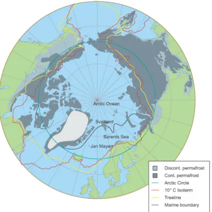
Figure 1-7 – Several definitions of the Arctic boundary: the Arctic Circle (green), the 10∘C summer isotherm (red), the tree line (yellow), the marine salinity boundary (black) and the location of permafrost (gray). Source: The Arctic System project, http://www. arcticsystem.no/en/arctic-inc/headquarters.html.
The Arctic region is traditionally defined as the region of the Northern Hemisphere where the 24-hour long polar day and polar night occur. This corresponds to the area north of the Arctic Circle, located at a latitude of 66°33′N. The Arctic can also be defined as the
area north of the tree line (the northern limit of tree growth), the area north of the 10∘C
summer surface isotherm, or other definitions based on the location of permafrost or on reduced ocean salinity. The Arctic boundaries corresponding to these definitions are shown
in Figure 1-7. In atmospheric studies, the Arctic is often more broadly defined as the area from 60∘N to 90∘N. This last definition is used in this thesis.
The Arctic is different from other regions because of several characteristics such as a high surface albedo due to sea ice, land ice and snow; long periods of darkness (polar night during winter) and sunlight (polar day during summer); high solar zenith angles; low temperatures; low relative humidities and strong atmospheric stability. The Arctic region is also especially sensitive to climate change (IPCC, 2013b).
1.2.2 Current Arctic warming
The Arctic surface is warming faster than the rest of the Earth (Figure 1-8(a)), a situation known as Arctic amplification. Arctic amplification was predicted using early climate model simulations (Kellogg, 1975; Manabe et al., 1990), and is mainly due to the positive surface-albedo climate feedback, combined with changes in heat transport to the Arctic, in Arctic clouds and in Arctic water vapor caused by climate change (Serreze and Barry, 2011). The enhanced radiative effects of black carbon aerosols in the Arctic are also thought to contribute to Arctic amplification (Serreze and Barry, 2011). This warming has important
(a) (b)
Figure 1-8 – (a) Annual mean Arctic surface temperature anomalies from 1880 to 2015 (blue), compared to the global average (black). Temperature anomalies are from the GISS surface temperature analysis (GISTEMP), and are relative to the 1951-1980 base period. (b) September Arctic sea ice cover, 1979-2015, with trend line (Figure from the National Snow and Ice Data Center, NSIDC).
consequences for the Arctic cryosphere. Figure 1-8(b) shows the evolution of September sea ice extent in the Arctic (when the yearly minimum cover is reached) between 1979 and 2015. Since satellite measurements began, September Arctic sea ice cover has declined at a rate of −13.4 % per decade (details in Stroeve et al., 2007). Arctic warming is also causing
the melt of the Greenland ice cap (−215 ± 59 Gt yr−1; IPCC, Vaughan et al., 2013), and
of Arctic glaciers (−138 ± 33 Gt yr−1, excluding Greenland; IPCC, Vaughan et al., 2013),
contributing to sea level rise. Snow cover is also declining in the Northern Hemisphere, by 1% to 2 % per year (IPCC, Vaughan et al., 2013).
1.2.3 Causes of Arctic warming
The Arctic is warming due to anthropogenic influences. Shindell et al. (2006) estimated that, during the 20thcentury, surface temperatures in the Arctic increased mostly because of
well-mixed greenhouse gases such as CO2 and CH4 (+1.65∘C). However, short-lived climate
forcers also appear to have played an important role (O3, +0.30
∘C; aerosols, including
sulfate, black carbon, organic carbon, and nitrate in air, BC on snow, and indirect effects, −0.76∘C). Shindell (2007) also found that aerosols and O3 have a stronger Arctic warming effect per unit forcing than well-mixed GHGs (see also Sections 2.1.7 and 2.2.5).
The literature review of Quinn et al. (2008) indicates that the direct effect of aerosols on Arctic surface temperatures is −0.98∘C, the indirect effect −0.70∘C and the snow albedo
effect (BC on snow) +0.043∘C. However, based on a multi-model analysis, AMAP (2015)
estimate that the direct effect of aerosols on Arctic surface temperatures is positive, +0.35∘C
(+0.40∘C from BC in air, +0.22∘C from BC in snow, and −0.27∘C from OC and SO4).
Re-sults from AMAP (2015) also indicate a weaker effect of O3 than previous studies, +0.12∘C.
Arctic warming is due to both local and remote forcings. Local forcings are due to the radiative effect of rising concentrations of greenhouse gases and aerosols within the Arctic, but Arctic warming can also be caused by remote forcings (located outside of the Arctic), which indirectly warm the Arctic through heat transport. Shindell (2007) estimated that most of the Arctic warming from 1880 to 2003 was caused by remote forcings, except during summer when local forcings made at least a similar contribution. However, Shindell and Faluvegi (2009) also showed that Arctic surface temperature was especially sensitive to local forcings, and dependent on the type of forcing.
1.2.4 Future projections
Future Arctic warming will depend on current and future action to limit climate change. Multi-model CMIP5 (Coupled Model Intercomparison Project Phase 5) future projections as part of the IPCC’s 5th assessment report (IPCC, 2013b) indicate that the Arctic will continue to warm the most, but that the magnitude of this warming will depend strongly on future emission pathways. For the lowest emission scenario used in the framework of CMIP5 (RCP2.6 scenario, Representative Concentration Pathway 2.6 W m−2), Arctic temperatures
are expected to rise by 2.2 ± 1.7∘C in 2100 compared to 1986-2005. In the highest emission
scenario (RCP8.5, Representative Concentration Pathway 8.5 W m−2), Arctic temperatures
As a result, in the RCP8.5 scenario most CMIP5 models predict an ice-free Arctic Ocean during summer (less than 1 × 10⁶km2 sea ice cover) by 2100. However, most models
under-estimate recent sea ice loss (Stroeve et al., 2007), and models which reproduce past changes the most indicate that the Arctic could be seasonaly ice-free in summer months before mid-century (Wang and Overland, 2012). Future Arctic warming is also expected to accelerate the loss of ice from ice sheets and glaciers, and contribute to sea-level rise. Under a medium-range warming scenario, Nick et al. (2013) predict that sea level will rise by 19 to 30 mm by 2200 due to the Greenland ice sheet alone.
1.3
Arctic air pollution
1.3.1 Arctic Haze
The Arctic troposphere was long thought to be extremely clean, until the 1950s, when pilots observed a reduction of visibility in the springtime North American Arctic (Greenaway, 1950; Mitchell, 1956). Further analysis showed that this Arctic Haze, which builds up every winter and spring, was of anthropogenic origin (Rahn et al., 1977). It contains enhanced levels of aerosols, mostly composed of sulphate and sea salt, as well as organic matter, nitrate and black carbon (Quinn et al., 2002). Arctic haze also contains elevated levels of several trace gases, such as carbon monoxide (CO), (NOx) and VOC (Solberg et al., 1996).
This peak in aerosol concentrations in late winter and early spring can be clearly seen in time series of aerosol measurements at Arctic surface stations. Figure 1-9, shows 1997-2004 and 1981–2003 sulfate and nitrate aerosol observations at Barrow (Alaska, USA) and Alert (Canada) (Quinn et al., 2007).
This Figure illustrates the strong seasonal variation of surface aerosol concentrations in the Arctic, reaching a maximum every year between January and April. These enhanced background levels at the surface (peaking below 2 km, Quinn et al., 2007) are called “Arctic Haze”. In addition to this background haze, the Arctic troposphere can be polluted by episodic transport events, which bring dense localized pollution plumes in the Arctic. These plumes should not strictly be called “Arctic Haze” but contribute to Arctic pollution (Brock et al., 2011).
1.3.2 Arctic air pollution transported from the mid-latitudes
In late winter and early spring, Eurasian pollution can be efficiently transported to the Arctic at low altitudes (Rahn, 1981), causing Arctic Haze. This strong influence of Eurasian emissions is due, in part, to the position of the Arctic front. Air masses traveling from the mid-latitudes to the Arctic usually rise along surfaces of constant potential temperature (isentropic transport). These surfaces form a fictional "dome" called the Arctic front, which
Figure 1-9 – Time-series of monthly averaged particulate sulfate and nitrate concentrations (in µgS m−3and µgN m−3respectively), at (a) Barrow, Alaska and (b) Alert, Canada. Figure
from Quinn et al. (2007).
isolates the lower Arctic troposphere from the mid-latitudes (Klonecki et al., 2003; Stohl, 2006). In addition, these rising air masses are usually associated with precipitation, which remove pollutants from the atmosphere (“wet removal”) during transport. On the contrary, pollutants emitted North of the Arctic front can be easily transported to the Arctic surface. Figure 1-10 shows the position of the Arctic front during winter and during summer, as well as the main atmospheric pathways from the mid-latitudes to the Arctic.
During winter and spring, the Arctic front can extend south down to 40∘N over Europe
and Russia due to the extensive snow cover and low temperatures there. Eurasian emissions within the Arctic front can then be transported into the lower Arctic troposphere. In winter and spring, pollution removal processes are also lower in Eurasia and in the Arctic due to strong atmospheric stability and reduced precipitation (Shaw, 1995; Garrett et al., 2011), causing the buildup of Arctic Haze. During summer, the Arctic front is located further north, and removal processes are higher, isolating the Arctic atmosphere from pollution in the mid-latitudes.
The main source regions of Arctic pollution are presented on Figure 1-11. This Figure shows the result of an earlier multi-model analysis (Shindell et al., 2008), estimating the rel-ative contributions of Europe, South Asia, East Asia, and North America to Arctic pollution at the surface and in the upper troposphere (250 hPa). These contributions were estimated for two aerosol components (BC and sulfate) and two trace gases (CO and ozone), by per-forming simulations with 20 % reduction in anthropogenic emissions of pollution precursors from each source region.
Figure 1-10 – Position of the Arctic front in winter (blue) and summer (yellow), and main pathways of atmospheric transport to the Arctic. From AMAP (2006).
Figure 1-11 – Relative importance of different source regions to annual mean Arctic con-centration at the surface and in the upper troposphere (250 hPa) for the indicated species. Arrow width is proportional to the multi-model mean percentage contribution from each region to the total from these four source regions. From Shindell et al. (2008).
pollution in the Arctic (blue arrows) are mostly influenced by European emissions. How-ever, Asian emissions play a more important role at higher altitudes (see also Fisher et al., 2011; Wang et al., 2014a). Figure 1-11 also indicates that, in these simulations, Arctic ozone is mostly sensitive to North American emissions, but Wespes et al. (2012) estimated that European anthropogenic emissions could have a similar or larger importance. Other model-ing studies have shown that, aside from anthropogenic emissions, Eurasian biomass burnmodel-ing could be a major source of Arctic pollution (Stohl, 2006; Warneke et al., 2010), but the scale of this contribution remains uncertain.
1.3.3 Developing local sources of Arctic pollution
Aerosols and ozone can be chemically destroyed or deposited during transport. These re-moval processes (described in Chapter 2) limit the efficiency of long-range transport of pollution from the mid-latitudes. Furthermore, pollution transport from the mid-latitudes occurs along rising isentrops, which tend to bring remote pollution at high altitudes in the Arctic (Stohl, 2006). Local Arctic emissions are, by definition, directly emitted in the Arctic boundary layer and do not experience aging during transport. For this reason, local sources can influence Arctic surface pollution (Sand et al., 2013) and Arctic pollution burdens (Wang et al., 2014a) with much higher per-emission efficiency than remote sources.
However, anthropogenic emissions in the Arctic are thought to be small compared to other regions. There are very few large cities north of the Arctic circle, the most populated being Murmansk in Russia ( ∼ 300,000 inhabitants); other large cities include Norilsk in Russia ( ∼ 175,000 inhabitants), Tromsø and Bodø in Norway ( ∼ 70,000 and 50,000 inhab-itants). There are some industrial sources of pollution north of the Arctic circle, such as mines and metal smelters in Norilsk, Russia (AMAP, 2006), and metal smelters in the Kola Peninsula, Russia (Prank et al., 2010). Oil and gas related activities in northern Russia and Norway (AMAP, 2006; Peters et al., 2011) are thought to be an important local source of Arctic pollution (especially for BC), and recent studies (Stohl et al., 2013; Huang et al., 2015) indicate that these emissions might be higher than previously thought.
Arctic shipping emissions are another noteworthy local source of pollution, emitting NOx,
SO2 (forming sulfate) and BC along with other pollutants. The Arctic council’s AMSA
report (Arctic Marine Shipping Assessment, Arctic Council, 2009) found that, in 2004, about 6000 ships operated within the Arctic (latitude > 60∘N). This traffic mostly takes
place along the Norwegian Coast, in northwestern Russia, around Iceland, in southwestern Greenland and in the Bering Sea. Arctic shipping is made up of a combination of supply ships for Arctic communities, bulk transport of resources extracted within the Arctic region, fishing ships, passenger ships and cruise ships (Arctic Council, 2009).
In addition to this local Arctic shipping, it has long been known that the routes through the Arctic Ocean are the shortest way from northern Europe and northwestern America
Figure 1-12 – Location of transit shipping routes through the Arctic (in red): Northern Sea Route (NSR, along the Russian coast) and Northwest Passage (NWP, along the Canadian coast). Adapted from IPCC (2014).
to Asia. For example, the Arctic route between the Netherlands and Eastern Asia (called the Northern Sea Route, NSR, or Northeast passage, NEP) is 40 % shorter than the corre-sponding route through the Suez Canal (Liu and Kronbak, 2010). The Arctic route from Northeastern America to Eastern Asia (the northwest passage, NWP) is 15 to 30 % shorter than the corresponding route through the Panama canal (Somanathan et al., 2009). These routes (shown in Figure 1-12) could be used to save trip distance and costs and might al-ready be profitable, but they are not widely used yet due to the presence of sea ice, leading to additional costs, additional risks due to potential ice damage, and reduced vessel speeds (Liu and Kronbak, 2010; Somanathan et al., 2009).
The NSR and NWP could become more economically competitive along with Arctic sea ice decline. Models and observations indicate that the number of ice-free days per year along the NSR and NWP increased by 22 and 19 days between 1979–1988 and 1998–2007 (Mokhov and Khon, 2008). As a result, transit along these routes is increasing: a record number of 71 ships transited through the NSR in 2013 (Northern Sea Route information office, 2013). At the same time, decreasing sea ice extent also contributed to a rise in Arctic cruise tourism (Stewart et al., 2009). The ice-free shipping season is expected to continue to lengthen due to climate change (Prowse et al., 2009; Khon et al., 2009). This will allow increased traffic along the NSR and NWP, by opening these routes to ships with no hull ice strengthening (Smith and Stephenson, 2013). As a result, Corbett et al. (2010) estimate that Arctic shipping emissions of NOxand BC could increase by a factor of 10 between 2004
and 2050 (high-growth scenario).
Increased shipping access in the Arctic is also expected to facilitate resource extraction in this region (Prowse et al., 2009). The Arctic contains vast resources of minerals (Lindholt, 2006), oil, and gas (Gautier et al., 2009). Arctic oil and gas resources are already being exploited, and the Arctic is expected to remain an important producer of oil by 2050, while its relative importance in gas production could decrease due to its high extraction prices (Lindholt and Glomsrød, 2012; Peters et al., 2011, projections shown in Figure 1-13). The oil and gas sector is expected to keep contributing to future local pollutant emissions in the Arctic (Peters et al., 2011), although current and future emission inventories from this source remain very uncertain.
Figure 1-13 – Historic and estimated oil (left) and gas (right) production in the Arctic, from 1960 to 2050. From Peters et al. (2011).
Local natural sources of aerosols, ozone and of their precursors in the Arctic are not well-known. They include boreal wildfires; sea salt, dimethylsulfide (DMS, forming sulfate) and organic matter from oceans; mineral dust; ozone transported from the stratosphere; NOx from soils and snow. Vegetation is sparse in the Arctic, which limits the formation
of biogenic VOCs from plants; and the lack of local thunderstorms (e.g., Cecil et al., 2014) prevents NOx formation from lightning. These natural sources are not the focus of this
thesis, but are included in the simulations presented in Chapter 4, 5 and 6 when estimates or emission models are available.
1.4
Scientific challenges in modeling Arctic aerosols and ozone
and their impacts
In this thesis, aerosol and ozone pollution in the Arctic is studied using regional simulations of the Arctic troposphere, and new global and local emission inventories of Arctic pollution. Model results are used to analyze recent aircraft measurements in the Arctic. This approach (details in Chapter 3) was motivated by results from previous studies, which showed that
modeling aerosol and ozone pollution in the Arctic was especially challenging.
1.4.1 Modeling aerosol and ozone pollution from long-range transport
Models do not represent aerosols well in the Arctic. Shindell et al. (2008) showed that models often underpredicted sulfate at Arctic surface stations, and greatly underpredicted BC, while several models struggled to reproduce the seasonal cycle of surface aerosol concentrations. Shindell et al. (2008) attributed this poor agreement to the treatment of aerosol aging and removal within models. Koch et al. (2009) and Schwarz et al. (2010) compared global models to different sets of aircraft observations of BC in the Arctic, and found that models underestimated BC at the surface but overestimated it aloft. A more recent intercomparison by Lee et al. (2013) also indicates that most models strongly underestimate surface BC observations in the Arctic, especially during winter and spring. Several studies (Huang et al., 2010; Liu et al., 2012; Browse et al., 2012; Wang et al., 2013) showed that Arctic BC could be improved by the use of more complex wet removal schemes within models. However, implementing these schemes does not fully resolve model disagreement with measurements (Browse et al., 2012; Wang et al., 2013, 2014b; Eckhardt et al., 2015).
Additionally, most models included in the recent intercomparison in the Arctic of Em-mons et al. (2015) underestimate ozone in the middle and high Arctic troposphere by ∼ 10 to 30 %, and exhibit stronger biases for ozone precursors such as NOx, carbon monoxide
(CO), peroxyacetyl nitrate (PAN) and several VOCs. Results from another recent model intercomparison in the Arctic performed by AMAP (Arctic Monitoring and Assessment Programme, AMAP, 2015) indicates that models are strongly biased for both O3 and its
precursors. These biases are attributed to uncertainties in emissions, errors in stratosphere-troposphere exchange and uncertainties related to the hydroxyl radical OH (these processes are described in Section 2.1).
1.4.2 Modeling aerosol and ozone pollution from local Arctic sources Emissions from local Arctic sources are not well quantified, which makes investigating their impacts difficult. There are very few specific emission inventories focused on local Arctic sources, and existing inventories are known to be incomplete. The current and future Arctic shipping inventories of Corbett et al. (2010) do not include fishing ships, which constitute a significant proportion of Arctic shipping (McKuin and Campbell, 2016). In addition, these inventories are based on the AMSA shipping dataset, which might underestimate Arctic marine traffic (Arctic Council, 2009). Other shipping inventories (Dalsøren et al., 2007, 2009; Peters et al., 2011) are also known to be biased towards specific ship types (i.e. container ships and large ships). Furthermore, Arctic shipping inventories can quickly become out of date as the local traffic increases and new emission control regulations are implemented (e.g., (Jonson et al., 2015)). A new Arctic shipping inventory based on ship
positioning by satellite was developed recently by Winther et al. (2014), but it has not yet been validated against measurements.
Emissions from the oil and gas sector are also very uncertain, as most oil and gas activity in the Arctic is located in northern Russia, where very few observations are available to validate inventories. Peters et al. (2011) estimated current and future emissions from Arctic oil and gas activities, but recent inventories (Huang et al., 2015; Klimont et al., 2015) indicate that this earlier estimate might be too low, especially in terms of BC emissions (Stohl et al., 2013).
For these reasons, earlier studies based on the inventories of Corbett et al. (2010), Dal-søren et al. (2007) and Peters et al. (2011), could be underestimating the impacts of Arctic shipping emissions. Furthermore, models do not represent well aerosol pollution in the Arc-tic. This could have a strong impact on results when studies report relative impacts of local emissions over this uncertain background.
Until recently, there was also no specific field measurements focused on Arctic shipping or Arctic resource extraction that could be used to study the impacts of local Arctic emissions, to assess model performance, and to validate inventories. Such a dataset is now available from the ACCESS aircraft campaign (Roiger et al., 2015), which took place in northern Norway in summer 2012 and specifically targeted ships and oil and gas platforms in the Norwegian and Barents seas.
Tropospheric ozone and tropospheric
aerosols in the Arctic
Aerosols and ozone are responsible for most of the health impacts of air pollution. They are also short-lived climate forcers. The processes governing aerosol and ozone pollution in the Arctic are complex, but underestanding these processes is critical in order to understand the impacts of Arctic aerosols and ozone on air quality and climate. This section presents the main chemical and physical processes governing ozone (Section 2.1) and aerosols (Section 2.2) in the troposphere, as well as their radiative impacts.
2.1
Tropospheric ozone
In this section, we only focus on the mechanisms which are the most important to understand ozone pollution in the Arctic (Jacob, 1999).
2.1.1 Introduction: stratospheric and tropospheric ozone
Ozone is a trace gas in the atmosphere, with mixing ratios ranging from 1 ppbv to 10 ppmv. The highest ozone concentrationss are found in the stratosphere between 20 to 30 km alti-tudes, a region known as the ozone layer (Figure 2-1) .
In the stratosphere, UV radiation (𝜆 < 240 nm) can dissociate O2 and form O3:
O2+ h𝜈−−−−−−−→ O(𝜆 < 240 nm 3P) + O(3P) (2.1)
O(3P) + O2+ M −−→ O3+ M (2.2)
Where O(3P) is the oxygen atom in its triplet state and M is a third body, usually O 2 or
N2. Reactions 2.1 and 2.2 produce O3, but O3 can also dissociate in the presence of UV
Figure 2-1 – Zonal mean ozone number concentrations (1979-2008 average), showing the location of the ozone layer around 25 km altitudes. Data from NOAA CDR (Bodeker et al., 2013).
radiation to make atomic oxygen, which can react with O3 to reform O2:
O3+ h𝜈−−−−−−−→ O𝜆 < 320 nm 2+ O(1D) (2.3)
O(1D) + M −−→ O(3P) + M (2.4)
O3+ O(3P) −−→ 2 O2 (2.5)
Where O(1D) is the oxygen atom in its singlet state. This cycle (2.1–2.5) is called the
Chapman cycle (Chapman, 1930). A steady-state analysis of this system reveals that it explains the location of the ozone layer, which is due to the simultaneous abundance of O2 and UV radiation (reaction 2.1) at altitudes 20 to 30 km (Chapman, 1930). At lower
altitudes, UV radiation at 𝜆 < 240 nm is filtered by the overhead O2 and O3, and reaction
2.1 cannot produce much O3.
However, O3 is also found at lower altitudes, in the troposphere (Figure 2-1). Since
high-energy UV radiation does not penetrate into the troposphere, it was once thought that tropospheric O3 was transported from the stratosphere. However, this theory could not
explain the observations of enhanced O3 at low altitudes and in polluted regions. Ripperton
et al. (1971); Chameides and Walker (1973); Crutzen (1974) later proved that O3 could also
be produced locally in the troposphere from natural and anthropogenic compounds.
2.1.2 Chemical O3 production in the troposphere from NOx and VOC
2.1.2.1 Ozone production from NO2
The main chemical reaction producing O3 in the troposphere is the photolysis of NO2:
NO2+ h𝜈−−−−−−−→ NO + O(𝜆 < 424 nm 3P) (2.6)
However, ozone can also react with NO to reform NO2:
NO + O3−−→ NO2 (2.8)
Reactions 2.6–2.7 and 2.8 are fast, and correspond to a quick interconversion between NO and NO2. For this reason, we can define the NOx chemical family as the sum NO + NO2.
This interconversion also means that ozone can only be produced in the troposphere from NO2 if there is another source of NO2 than reaction 2.8.
2.1.2.2 Oxidation of CO, CH4 and other hydrocarbons as ozone sources
Earlier studies identified that NO2could be produced in the troposphere during the oxidation
of CO (Levy, 1972):
CO + OH −−→ CO2+ H (2.9)
H + O2+ M −−→ HO2+ M (2.10)
HO2+ NO −−→ NO2+ OH (2.11)
Where OH is the hydroxyl radical and HO2 the hydroperoxyl radical. Similarly to NOx, a
HOxfamily can be defined as OH+HO2. OH can be produced in the troposphere by several
photochemical reactions, notably:
O3+ h𝜈−−−−−−−→ O𝜆 < 320 nm 2+ O(1D) (2.12)
O(1D) + H2O −−→ 2 OH (2.13)
Reaction 2.12 can occur from photons at wavelengths 300 nm < 𝜆 < 320 nm, which are found in the troposphere (photons at 𝜆 < 300 nm are filtered by overhead stratospheric O3 and O2). From reactions 2.12–2.13, one O3 molecule can produce 2 OH molecules, and
each OH molecule can form one NO2 molecule by oxidizing CO (2.9). This can result in net
O3 production if other reactions do not consume HOx or NO2. OH is an especially critical
compound in the troposphere, since it controls the lifetime of a large number of tropospheric trace gases such as CO. For example, OH can also oxidize hydrocarbons such as CH4:
CH4+ OH −−→ CH3+ H2O (2.14)
CH3+ O2+ M −−→ CH3O2+ M (2.15)
CH3O2+ NO −−→ CH3O + NO2 (2.16)
Reactions 2.14–2.16 provide another source of NO2 which can potentially produce O3.
Fur-thermore, the methyl peroxy radical, CH3O2, can be oxidized to form methoxy radicals,
CH3O, and formaldehyde, CH2O (details in Jacob, 2000). Under high NOx, these pathways
lead to the formation of additional HO2 and CO, and one molecule of CH4 can produce an
these additional reactions are a net sink of HOx and can decrease O3. Longer hydrocarbon
chains R−H can also be oxidized by a mechanism similar to 2.14–2.16 to form RO2 and
NO2. Organic compounds present in the gas phase in the atmosphere are called Volatile
Organic Compounds (VOC).
2.1.2.3 Global emissions of NOx, CO, CH4 and non-methane VOC (NMVOC)
Tropospheric O3 is produced from NOx, CO, CH4, and other (non-methane) VOC. At the
global scale, the main source of NOx and CO is human activity (Table 2.1). Natural emis-sions of NOx are due to soils, lightning and wildfires. VOC emissions are mostly natural,
due to methane sources from wetlands, and emissions of isoprene and terpenes by vegeta-tion. Human VOC emissions include methane, several alkanes and alkenes, and aromatic compounds such as benzene and toluene. The non-methane VOC category represents a large variety of compounds with different reactivities and different impacts on ozone production. Table 2.1 – Global NOx, CH4 and NMVOC emissions by source, from IPCC (Ciais et al.,
2013; IPCC, 2013a), Wiedinmyer et al. (2011) and Sindelarova et al. (2014)
Source NOx CH4 CO NMVOC
(TgN yr−1) (Tg yr−1) (Tg yr−1) (Tg yr−1)
Anthropogenic, excluding agriculture 28.3 96 1071 213
Agriculture 3.7 204.5 -
-Biomass burning 5.5 32.5 372.5 81.3
Soils 7.3 - -
-Lightning 4 - -
-Vegetation - - - 950
Oceans and geological sources - 54 49 4.9
Wetlands, other natural sources - 228.5 -
-2.1.3 Photochemical sinks of ozone, HOx and NOx in the troposphere
The main chemical sinks of ozone in the troposphere are the following reactions:
O3+ h𝜈 −−→ O2+ O(1D) (2.12)
O(1D) + H2O −−→ 2 OH (2.13)
O3+ OH −−→ O2+ HO2 (2.17)
O3+ HO2 −−→ OH + 2 O2 (2.18)
In addition, since there is an interconversion between O3, NO2 and HOx, loss of HOx and