Validation of a method to compensate multicenter effects affecting CT radiomic features

(1)

HAL Id: hal-01953538

https://hal.archives-ouvertes.fr/hal-01953538

Submitted on 13 Dec 2018

HAL is a multi-disciplinary open access

archive for the deposit and dissemination of sci-entific research documents, whether they are pub-lished or not. The documents may come from teaching and research institutions in France or abroad, or from public or private research centers.

L’archive ouverte pluridisciplinaire HAL, est destinée au dépôt et à la diffusion de documents scientifiques de niveau recherche, publiés ou non, émanant des établissements d’enseignement et de recherche français ou étrangers, des laboratoires publics ou privés.

Validation of a method to compensate multicenter

effects affecting CT radiomic features

Fanny Orlhac, Frédérique Frouin, Christophe Nioche, Nicholas Ayache, Irene

Buvat

To cite this version:

Fanny Orlhac, Frédérique Frouin, Christophe Nioche, Nicholas Ayache, Irene Buvat. Validation of a method to compensate multicenter effects affecting CT radiomic features. Radiology, Radiological Society of North America, In press. �hal-01953538�

(2)

Validation of a method to compensate multicenter effects affecting CT radiomic

Fanny Orlhac (PhD)1_{, Frédérique Frouin (PhD)}2_{, Christophe Nioche (PhD)}2_, Nicholas Ayache (PhD)1_{, Irène Buvat (PhD)}2

1: UCA, Inria Sophia Antipolis – Méditerranée, Epione, 2004 route des Lucioles – BP 93, 06 902 Sophia Antipolis Cedex, France.

2: Imagerie Moléculaire In Vivo, CEA-SHFJ, Inserm, CNRS, Université Paris-Sud, Université Paris-Saclay, 4 place du Général Leclerc, 91 400 Orsay, France.

Corresponding author:

Fanny Orlhac +33 4 92 38 71 52 [email protected]

Inria Sophia Antipolis – Méditerranée 2004 route des Lucioles – BP 93 06 902 Sophia Antipolis Cedex, France

Article type: Technical Development Word count: 2510 words

(3)

List of all abbreviations:

ABS: Acrylonitrile Butadiene Styrene CCR: Credence Cartridge Radiomics FBP: Filtered Back Projection L: Lung reconstruction algorithm PCA: Principal Component Analysis

RIDER: Reference Image Database to Evaluate therapy Response S: Standard reconstruction algorithm

S3: Sinogram affirmed iterative reconstruction with a noise reconstruction strength of level 3 S5: Sinogram affirmed iterative reconstruction with a noise reconstruction strength of level 5 VOI: Volume of Interest

(4)

Abstract

Purpose: We investigated whether a compensation method could correct for the variations of radiomic

feature values caused by the use of different CT protocols.

Materials and Methods: Phantom data involving 10 texture patterns and 74 patients (cohort #1: 42

patients; 19 males; mean age, 60.4 years; range, 31-81 years; September-October 2013; cohort #2: 32 patients; 16 males; mean age, 62.1 years; range, 29-82 years; January-September 2007) scanned using different CT protocols were retrospectively included. For any radiomic feature, the compensation approach identified a protocol-specific transformation to express all data in a common space devoid of protocol effects. The differences in statistical distributions between protocols were assessed using Friedman tests before and after compensation. Principal component analyses (PCA) were performed on the phantom data to evaluate the ability to distinguish between texture patterns after compensation.

Results: In the phantom data, the statistical distributions of features were different between protocols for

all radiomic features and texture patterns (p<.05). After compensation, the protocol effect was no longer detectable (p>.05). PCA demonstrated that each texture pattern was no longer displayed as different clusters corresponding to different imaging protocols unlike what was observed before compensation. The correction for scanner effect was confirmed in patient data with 100% (10/10 features for cohort #1) and 98% (87/89 features for cohort #2) of p-values less than .05 before compensation, compared to 30% (3/10) and 15% (13/89) after compensation.

Conclusion: The compensation successfully realigns feature distributions computed from different CT

(5)

Introduction

Since 2012, the concept of Radiomics is expanding (1) in oncology with the objective to characterize tumor heterogeneity from medical images. Radiomics extracts features from medical images that quantify tumor shape, intensity histogram and texture of the lesions more precisely and more accurately than visual assessment by a radiologist, in order to build models involving such features to assist patient management. In particular, texture analysis from CT images has led to promising results to distinguish between tumor lesions with different histopathological characteristics and to predict treatment response or patients survival (2). However, several studies have highlighted the sensitivity of radiomic features to CT acquisition and reconstruction parameters using phantoms (3–8) or patient data (9–12). Indeed, feature values are affected by slice thickness, pixel size, reconstruction kernel, tube voltage, tube current and contrast-enhancement. They also differ between different scanners with the same settings (8). Moreover, the impact of imaging protocols varies according to the texture pattern and the radiomic feature (4).

One of the most widely cited studies in radiomics (13), which included 1019 patients, used different CT imaging protocols involving different CT scanners, different pixel size and slice thickness, with or without intravenous contrast, without accounting for this variability in the data analysis. To reduce that variability, it has been proposed to resample images with a fixed voxel size, to filter the images (5) or to change the definition of features (6,11). These approaches require a modification of the CT images or are not applicable to all radiomic features.

The same issue is encountered in PET imaging, where radiomic features are sensitive to the acquisition protocol and reconstruction algorithm (14). A compensation method was initially described in genomics (15), where the so-called batch effect is the source of variations in measurements caused by the handling of samples by different laboratories, different technicians and on different days. The batch-effect is conceptually similar to variations induced by the scanner or the protocol effects in radiomics. The

(6)

compensation method identifies a batch-specific transformation to express all data in a common space devoid of batch effects. It has been shown to be effective in PET to realign the radiomic feature distributions between 3 different protocols for healthy liver tissue and breast lesions, without altering the biological information (16).

The purpose of this study was therefore to determine whether this compensation method could also correct for the CT protocol effect, using phantom and patient data.

Materials and Methods

All patient data were anonymized and publicly available in supplemental data of (9) and (10). All authors had control of the data and information submitted for publication.

Phantom experiments

The phantom data used in our study have been produced by Mackin et al (4) and are publicly available in supplemental data of (4). The Credence Cartridge Radiomics (CCR) phantom consists of 10 layers with different materials corresponding to different texture patterns. This phantom was scanned using 17 different imaging protocols from four medical institutes involving various reconstruction kernels, scan types, slice thickness, pixel spacing, spiral pitch factor and effective milliamperage. Additional information on phantom and acquisition characteristics are provided in Supplemental Tables 1 and 2. For each layer, 16 non-overlapping volumes of interest (VOI) with a cubic volume, on average, of 8 cm3_{(range: [7.6 - 9} cm3_{] corresponding to [2708 - 14332 voxels] depending on the imaging protocols) are also made available} in Dicom-RTstruct format. For each VOI and each imaging protocol, we (FO with 7 years and CN with 20 years of research experience in medical imaging) computed 40 radiomic features using the LIFEx freeware (17) (www.lifexsoft.org, Inserm, Orsay, France, Supplemental Table 3), with a fixed bin size (18) set to 10

(7)

HU between -1 000 UH and 3 000 UH without any spatial resampling. We performed the radiomic analysis for 16 imaging protocols out of 17 due to a reading issue with acquisition CCR1-GE2.

Patients

Publicly available radiomic features from two patient databases (#1 and #2) were used in our study. First set of features was derived from cohort #1 of 42 patients with a lung cancer between September and October 2013 (9), including 19 males (mean age, 60.4 years; range, 31-81 years, Table 1). All patients underwent a CT scan with the same machine and protocol (Supplemental Table 4), and CT images were reconstructed using three algorithms: filtered back projection (FBP), Sinogram Affirmed Iterative Reconstruction (Siemens Healthcare, Forchheim, Germany) with a noise reduction strength of level 3 (called S3 thereafter) and 5 (called S5). For each patient, the dominant tumor lesion was segmented manually three times, twice by a radiologist and once by a technologist. For each of the 3 VOIs per patient and each reconstruction, 15 radiomic features were calculated. We (FO) excluded 5 geometric features (volume, diameter, surface, sphericity and compactness) from the analysis as they mostly depend on the segmentation.

Second set of features was obtained from 32 patients of cohort #2 between January and September 2007 (16 males; mean age, 62.1 years; range, 29-82 years, Table 1) with a lung cancer who underwent two CT scans (Supplemental Table 4) within 15 minutes (10). This dataset was originally collected in the clinical trial NCT00579852 to evaluate the reproducibility of tumor volume and diameter measurements and is part of the Reference Image Database to Evaluate therapy Response (RIDER) project (19). The CT images were reconstructed using 6 protocols combining two reconstruction algorithms (lung and standard abbreviated as L and S) and three slice thicknesses (1.25 mm, 2.5 mm and 5 mm) (10). For one lesion per patient (29 primary and 3 metastatic lesions), a tumor VOI was obtained from a consensus among the

(8)

manual segmentations by 3 radiologists. After resampling the VOI voxels to 0.5x0.5x0.5 mm3 _{using a} tri-linear interpolation, 89 radiomic features were calculated for the 6 imaging protocols (2 reconstructions x 3 slice thicknesses) and for each of the 64 scans (32 patients with 2 scans).

Compensation method

To correct for differences in features caused by the various imaging protocols, we (FO) used the ComBat compensation method (15). This method has been used for cortical-thickness measurements from MR images (20) and for radiomic features from different PET protocols (16). It is a data-driven method that identifies the protocol effect assuming that the value of each feature y measured in VOI j with imaging protocol i can be written as:

yij=α+ γi+δiεij Equation 1

where α is the average value for feature yij, γi is an additive protocol effect, and δi is a multiplicative

protocol effect affected by an error term (εij). The compensation consists in estimating the model

parameters α, γi and δi using a maximum likelihood approach based on the set of available observations

y:

yijComBat=

yij-α̂-γ̂i

δ̂i +α̂ Equation 2

where α̂, γ̂ and δi ̂ are estimators of α, γi i and δi.

We used the non-parametric form of the model in which no assumptions are made regarding the laws followed by the parameters. In this setting, ComBat determines a transformation for each feature separately. For each texture pattern of phantom data and of each patient dataset, we used the R (version

(9)

3.4.2, R foundation for Statistical Computing, Vienna, Austria) function called ComBat, available at https://github.com/Jfortin1/ComBatHarmonization to identify the transformation parameters.

Statistical analysis

To determine whether the protocol setting (independent variable i in Equation 1) impacted the distributions of radiomic feature values (dependent variables yij in Equation 1), we (FO, FF with 30 years of experience) performed 2-sided Friedman tests before and after ComBat compensation for each feature as summarized in Supplemental Table 5. Null hypothesis is that there is no difference between the distributions. Benjamini-Hochberg procedure was used to control the false discovery rate (21). P-values less than .05 were regarded as statistically significant. As the goal of the compensation is to realign the distributions in terms of mean and standard deviation, a p-value of the Friedman test greater than .05 means that the realignment was successful.

For the phantom data, we also performed a principal component analysis (PCA) of the 2 560 samples (16 VOI x 10 texture patterns x 16 imaging protocols) described by 40 variables (radiomic features). PCA was performed before and after ComBat to visualize the impact of the compensation method on the distinction between patterns. We also studied whether two textural patterns could be distinguished when pooling data from the 3 imaging protocols before and after compensation and for balanced and un-balanced groups.

(10)

Results

Patient characteristics are shown in Table 1.

Phantom experiments

In the phantom data, 399/400 p-values of the Friedman tests performed for all features based on 16 imaging protocols and 10 texture patterns were lower than .05 before compensation (Table 2, Supplemental Table 6). Only one p-value for Skewness was larger than .05 for pattern 7 (dense cork, p=.46). After compensation, all p-values of Friedman tests were higher than .05, demonstrating that the protocol effect was no longer detectable.

These results were confirmed visually using the projection of the data in the space spanned by the first 2 principal components of PCA. Figure 1 shows an overlapped between textural patterns before ComBat, due to the large variability of radiomic feature values computed from 16 different CT protocols. For each textural pattern (each color), several clusters corresponding to different CT protocols could be identified. After ComBat, textural patterns could be clearly distinguished and were no longer composed of different clusters, demonstrating that the compensation method properly corrected for the scanner effect while retaining the specific characteristics of each texture pattern. Interestingly, the variance explained by the first two components was higher after ComBat (65.6% versus 53.2%), with approximately the same features contributing to the first two principal components before and after compensation (data not shown).

Based on three CT acquisitions (GE1, P2 and S2, see Supplemental Table 2), Figure 2 shows that when data were pooled without realignment, the sensitivity for distinguishing cork from dense cork was 67% (32/48 VOI) with a specificity of 98% (47/48 VOI) using the cutoff maximizing the Youden index. After ComBat, both sensitivity and specificity were 100% (48/48 VOI). For unbalanced groups, Supplemental Figure 1 shows that the compensation method also yielded a perfect distinction between these two patterns.

(11)

Patient data

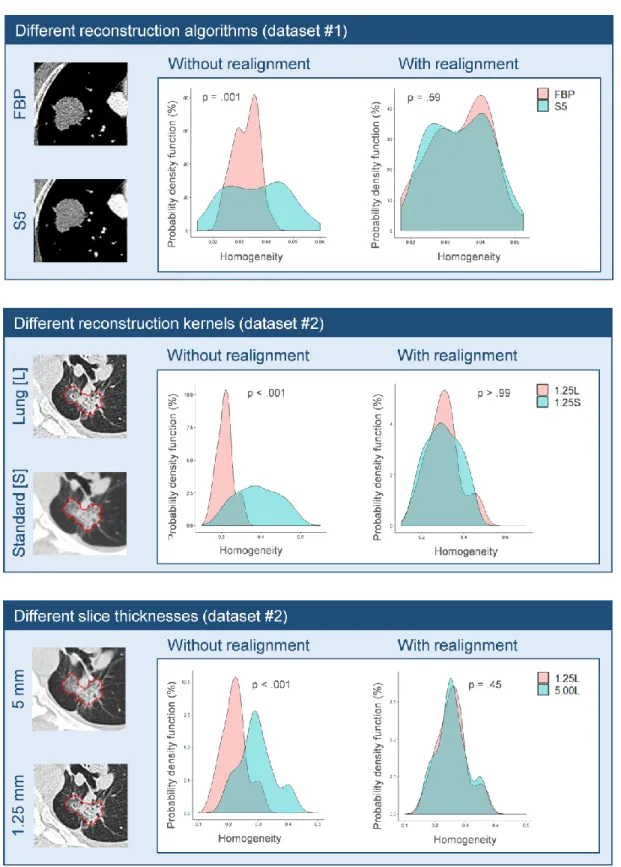
For patient datasets #1 and #2, 100% (10/10) and 98% (87/89) of Friedman tests respectively were lower than .05 between imaging protocols before ComBat (Table 2, Supplemental Tables 7-8). After ComBat, 30% (3/10) of p-values for dataset #1 and 15% (13/89) of p-values for dataset #2 were lower than .05. Visual inspection of the radiomic feature value distributions when Friedman tests remained significant after ComBat showed that the residual difference between protocols was always small and that the protocol effect was much reduced (Supplemental Figure 2), demonstrating the effectiveness of the compensation. As illustrated in Supplemental Figure 3 for Homogeneity feature, ComBat corrects the protocol effect with a realignment of feature values among the three protocols for dataset #1 and among the 6 protocols for dataset #2. For instance, before ComBat, the plot shows a shift in distribution with greater Homogeneity values for reconstruction S5 than for S3 and FBP. This was expected since S5 involved higher noise reduction. After compensation, the distributions between the three reconstructions better overlapped. Figure 3 shows three examples of realignment of features between different reconstruction algorithms, reconstruction kernels and slice thicknesses.

Discussion

As widely reported in the literature, radiomic features are sensitive to the acquisition and reconstruction parameters of CT images. Feature values are therefore not directly comparable between different imaging protocols, limiting their use in multicenter studies. Here, we demonstrated that the ComBat method can realign radiomic features computed from different CT imaging protocols. Using phantom data, we showed that ComBat removed the scanner and protocol effect while preserving the differences between texture patterns. The correction for the scanner effect was confirmed using patient images reconstructed with different imaging protocols.

(12)

The use of this compensation method should facilitate multicentric radiomic analyses that are absolutely needed to demonstrate the practical usefulness of radiomic features for patient management. Data harmonization is currently a hot topic in the international imaging community with increasing awareness of the need to reduce the variability in image quality between centers and machines (22,23). ComBat offers a solution to realign radiomic features with several advantages. ComBat is easily available to all and fast (a function available for free in R software). The transformations are estimated based on the measured feature values, without the need to go back to images or to perform phantom experiments. No learning set is needed. Unlike other options described in the literature, ComBat does not change the feature definitions (6,11) and can therefore be used with all software/algorithms and with any radiomic features. This is illustrated in three datasets using three different implementations for the radiomic feature calculation (Supplemental Table 5). ComBat does not require spatial resampling of the CT images to a single pixel size and/or image filtering (5). It is applicable when only radiomic features values are available or when images are not available. ComBat can account for covariates of interest if the patients scanned with different imaging protocols do not have the same characteristics (eg, different age distributions). ComBat can model these covariates in the compensation process as illustrated in PET imaging with different proportions of cancer subtypes in different departments (16), as long as enough patients with the same characteristics are available.

As demonstrated using the phantom data (Table 2), before compensation, the values of radiomic features were significantly different between imaging protocols for a given pattern. Ignoring this effect in multicentric studies might bias the findings and lower statistical power. A recent study highlighted that the 4 features selected in (13) to build the radiomic signature were highly correlated with tumor volume (24), which might explain why the model remained robust on data from different centers. Using ComBat might help determine whether radiomic features reflecting the lesion biological heterogeneity but affected by the center effect more than the lesion volume also have some predictive value.

(13)

Our study has some limitations: our findings should be confirmed on other cancer types, for other imaging protocols and scanners and the actual impact on diagnostic performance on clinical data needs to be demonstrated. Independent multi-center validation of radiomic models is also essential for them to become mainstream (1,25,26).

In summary, ComBat makes it possible to pool radiomic features from different CT protocols. This method appears promising to deal with the center effect in multicenter radiomic studies and to possibly raise the statistical power of such studies. ComBat is data-driven meaning that the transformations identified by ComBat to set all data in a common space should be estimated for each study involving data from different centers/protocols. Our analysis was based on less than 50 patients for each acquisition protocol demonstrating the efficiency of the method even for small patient cohorts. Using simulations in which we gradually removed patient data (results not shown), we found satisfactory results with as few as 20 patients per imaging protocol. The minimum number of patients required per imaging protocol to successfully apply ComBat remains to be comprehensively investigated.

(14)

References

1. Gillies RJ, Kinahan PE, Hricak H. Radiomics: Images Are More than Pictures, They Are Data.

Radiology. 2016;278(2):563–577. doi: 10.1148/radiol.2015151169.

2. Lubner MG, Smith AD, Sandrasegaran K, Sahani DV, Pickhardt PJ. CT Texture Analysis: Definitions, Applications, Biologic Correlates, and Challenges. Radiographics. 2017;37(5):1483–1503. doi: 10.1148/rg.2017170056.

3. Zhao B, Tan Y, Tsai WY, Schwartz LH, Lu L. Exploring Variability in CT Characterization of Tumors: A Preliminary Phantom Study. Transl Oncol. 2014;7(1):88–93. doi: 10.1016/j.tranon.2014.09.001.

4. Mackin D, Fave X, Zhang L, et al. Measuring Computed Tomography Scanner Variability of Radiomics Features. Invest Radiol. 2015;50(11):757–765. doi: 10.1097/RLI.0000000000000180.

5. Mackin D, Fave X, Zhang L, et al. Harmonizing the pixel size in retrospective computed tomography radiomics studies. PLoS ONE. 2017;12(9):e0178524. doi: 10.1371/journal.pone.0178524.

6. Shafiq-Ul-Hassan M, Zhang GG, Latifi K, et al. Intrinsic dependencies of CT radiomic features on voxel size and number of gray levels. Med Phys. 2017;44(3):1050–1062. doi: 10.1002/mp.12123.

7. Caramella C, Allorant A, Orlhac F, et al. Can we trust the calculation of texture indices of CT images? A phantom study. Med Phys. 2018;45(4):1529–1536. doi: 10.1002/mp.12809.

8. Berenguer R, Pastor-Juan MDR, Canales-Vázquez J, et al. Radiomics of CT Features May Be Nonreproducible and Redundant: Influence of CT Acquisition Parameters. Radiology. 2018;288(2):407–415. doi: 10.1148/radiol.2018172361.

9. Kim H, Park CM, Lee M, et al. Impact of Reconstruction Algorithms on CT Radiomic Features of Pulmonary Tumors: Analysis of Intra- and Inter-Reader Variability and Inter-Reconstruction Algorithm Variability. PLoS ONE. 2016;11(10):e0164924. doi: 10.1371/journal.pone.0164924.

10. Lu L, Ehmke RC, Schwartz LH, Zhao B. Assessing Agreement between Radiomic Features Computed for Multiple CT Imaging Settings. PLoS ONE. 2016;11(12):e0166550. doi: 10.1371/journal.pone.0166550.

11. Shafiq-Ul-Hassan M, Latifi K, Zhang G, Ullah G, Gillies R, Moros E. Voxel size and gray level

normalization of CT radiomic features in lung cancer. Sci Rep. 2018;8(1):10545. doi: 10.1038/s41598-018-28895-9.

12. He L, Huang Y, Ma Z, Liang C, Liang C, Liu Z. Effects of contrast-enhancement, reconstruction slice thickness and convolution kernel on the diagnostic performance of radiomics signature in solitary pulmonary nodule. Sci Rep. 2016;6:34921. doi: 10.1038/srep34921.

13. Aerts HJWL, Velazquez ER, Leijenaar RTH, et al. Decoding tumour phenotype by noninvasive imaging using a quantitative radiomics approach. Nat Commun. 2014;5:4006. doi:

10.1038/ncomms5006.

14. Yan J, Chu-Shern JL, Loi HY, et al. Impact of Image Reconstruction Settings on Texture Features in 18F-FDG PET. J Nucl Med. 2015;56(11):1667–1673. doi: 10.2967/jnumed.115.156927.

(15)

15. Johnson WE, Li C, Rabinovic A. Adjusting batch effects in microarray expression data using empirical Bayes methods. Biostatistics. 2007;8(1):118–127. doi: 10.1093/biostatistics/kxj037.

16. Orlhac F, Boughdad S, Philippe C, et al. A Postreconstruction Harmonization Method for Multicenter Radiomic Studies in PET. J Nucl Med. 2018;59(8):1321–1328. doi:

10.2967/jnumed.117.199935.

17. Nioche C, Orlhac F, Boughdad S, et al. LIFEx: A Freeware for Radiomic Feature Calculation in Multimodality Imaging to Accelerate Advances in the Characterization of Tumor Heterogeneity. Cancer Res. 2018;78(16):4786–4789. doi: 10.1158/0008-5472.

18. Orlhac F, Soussan M, Chouahnia K, Martinod E, Buvat I. 18F-FDG PET-Derived Textural Indices Reflect Tissue-Specific Uptake Pattern in Non-Small Cell Lung Cancer. PLoS ONE.

2015;10(12):e0145063. doi: 10.1371/journal.pone.0145063.

19. Armato SG, Meyer CR, Mcnitt-Gray MF, et al. The Reference Image Database to Evaluate Response to therapy in lung cancer (RIDER) project: a resource for the development of change-analysis software. Clin Pharmacol Ther. 2008;84(4):448–456. doi: 10.1038/clpt.2008.161.

20. Fortin J-P, Cullen N, Sheline YI, et al. Harmonization of cortical thickness measurements across scanners and sites. Neuroimage. 2018;167:104–120. doi: 10.1016/j.neuroimage.2017.11.024.

21. Benjamini Y, Hochberg Y. Controlling the False Discovery Rate: A Practical and Powerful Approach to Multiple Testing. Journal of the Royal Statistical Society Series B (Methodological).

1995;57(1):289–300. doi: 10.2307/2346101.

22. Sullivan DC, Obuchowski NA, Kessler LG, et al. Metrology Standards for Quantitative Imaging Biomarkers. Radiology. 2015;277(3):813–825. doi: 10.1148/radiol.2015142202.

23. O’Connor JPB, Aboagye EO, Adams JE, et al. Imaging biomarker roadmap for cancer studies. Nat Rev Clin Oncol. 2017;14(3):169–186. doi: 10.1038/nrclinonc.2016.162.

24. Vallieres M, Visvikis D, Hatt M. Dependency of a validated radiomics signature on tumor volume and potential corrections. J Nucl Med. 2018;59(supplement 1):640–640.

http://jnm.snmjournals.org/content/59/supplement_1/640

25. Buvat I, Orlhac F, Soussan M. Tumor Texture Analysis in PET: Where Do We Stand? J Nucl Med. 2015;56(11):1642–1644. doi: 10.2967/jnumed.115.163469.

26. Reuzé S, Schernberg A, Orlhac F, et al. Radiomics in Nuclear Medicine Applied to Radiation Therapy: Methods, Pitfalls, and Challenges. Int J Radiat Oncol Biol Phys. 2018;102(4):1117–1142. doi:

(16)

Table 1: Patient characteristics.

Patient dataset #1 Patient dataset #2

Sex-no. (%) Male 19 (45%) 16 (50%) Female 23 (55%) 16 (50%) Age-yr. Mean 60.4 62.1 Range 31-81 29-82 Lesion-no. (%)

Primary lung lesion 8 (19%) 29 (91%)

(17)

Table 2: number of significant Friedman tests (p<.05) without and with compensation in the phantom

and clinical datasets.

w/o realignment with realignment

Phantom (40 tests for each pattern)

Pattern 1: 20% filled ABS 40/40 (100%) 0/40 (0%)

Pattern 5: acrylic 40/40 (100%) 0/40 (0%)

Pattern 6: cork 40/40 (100%) 0/40 (0%)

Pattern 7: dense cork 39/40 (98%) 0/40 (0%)

Pattern 8: plaster resin 40/40 (100%) 0/40 (0%)

Pattern 9: rubber particles 40/40 (100%) 0/40 (0%)

Pattern 10: wood 40/40 (100%) 0/40 (0%)

Patient dataset #1 (10 tests) 10/10 (100%) 3/10 (30%)

Patients dataset #2 (89 tests) 87/89 (98%) 13/89 (15%)

(18)

Figure 1: Phantom data: principal component scores for 2560 samples corresponding to 16 VOI x 10

texture patterns (in colors) x 16 imaging protocols described by 40 radiomic features on the first two principal components before (A) and after ComBat (B). After compensation, each texture pattern was no longer composed of different clusters, demonstrating that the scanner effect has been correctly

(19)

Figure 2: Example of ComBat application in phantom experiments: two texture patterns (cork and dense

cork) were scanned using three different imaging protocols with 16 volumes of interest in each case (GE1, P2, S2, see Supplemental Table 2). When pooling all radiomic feature values, the optimal cutoff could not perfectly distinguish the patterns while after compensation of scanner effects, a perfect distinction was observed.

(20)

Figure 3: Probability density function(%) of Homogeneity before (left) and after ComBat (right) in patient

data using two CT reconstruction algorithms (FBP and S5), two reconstruction kernels (Standard and Lung) and two voxel thicknesses (1.25 mm and 5 mm). CT images are from Kim et al, PLoS ONE

2016;11:e0164924 and Lu et al, PLoS ONE 2016;11:e0166550. Displayed p-values are given for Friedman tests.

(21)

Supplemental Figure 1: Phantom experiments: distinction between two patterns (Cork vs Dense cork)

for 3 acquisition protocols with unbalanced groups (different numbers of cork and dense cork VOI for each scanner) without and with realignment.

(22)

Supplemental Figure 2: Probability density function of 4 radiomic features before (left) and after (right)

ComBat for patient dataset #1 (A, B) and #2 (C, D). For these features, the p-values of Friedman test remained statistically significant after ComBat but these plots demonstrate that the correction was effective.

(23)

Supplemental Figure 3: Boxplot before (left) and after (right) compensation for the homogeneity

feature. A) patient dataset #1 for 3 reconstruction algorithms (FBP, S3 and S5). B) patient dataset #2 for 6 different protocols involving three slice thicknesses (1.25 mm, 2.5 mm and 5 mm) and two

(24)

Supplemental Table 1: phantom characteristics.

No. Description Illustration

Pattern 1 Acrylonitrile butadiene styrene (ABS) plastic with 20% of air-filled (holes of

diameter = 6.0 mm)

Pattern 2 ABS plastic with 30% of air-filled (holes of diameter = 1.4 mm)

Pattern 5 Solid polymethyl methacrylate (acrylic)

Pattern 6 Standard cork

Pattern 7 Dense cork

Pattern 8 Plaster resin

Pattern 9 Rubber particles

(25)

Supplemental Table 2: acquisition characteristics for phantom experiments.

Designation Manufacturer/Model Reconstruc tion kernel

Scan

type Voxel size (mm3)

Spiral pitch factor

kVp mAs

GE1 GE/Discovery CT750 HD standard helical 0.49x0.49x2.5 0.98 120 81

GE3 GE/Discovery CT750 HD standard helical 0.78x0.78x2.5 0.98 120 122

GE4 GE/Discovery ST standard helical 0.98x0.98x2.5 1.35 120 143

GE5 GE/LightSpeed RT standard helical 0.98x0.98x2.5 0.75 120 1102

GE6 GE/LightSpeed RT16 standard helical 0.98x0.98x2.5 0.94 120 367

GE7 GE/LightSpeed VCT standard helical 0.74x0.74x2.5 0.98 120 82

P1 Philips/Brilliance Big Bore B helical 0.98x0.98x3 0.94 120 320

P2 Philips/Brilliance Big Bore C helical 0.98x0.98x3 0.94 120 369

P5 Philips/Brilliance 64 B helical 0.98x0.98x3 0.67 120 372

S1 Siemens/Sensation Open B31s axial 0.52x0.52x2 1.00 120 26-70

S2 Siemens/Somatom Definition Flash 170f, 2 helical 0.54x0.54x3 0.60 120 17-28

T1 Toshiba/Aquilion FC18 helical 0.63x0.63x3 1.11 120 135

T2 Toshiba/Aquilion FC18 helical 0.63x0.63x3 1.11 120 135

(26)

Supplemental Table 3: list of radiomic features extracted from phantom data. Complete description is

available on www.lifexsoft.org.

Category Features

Histogram Mean, Standard-Deviation, Maximum, Skewness, Kurtosis, Entropy (log2 and log10), Energy

Gray-Level Co-occurrence Matrix

(GLCM)

Homogeneity, Energy, Contrast, Correlation, Entropy (log2 and log10), Dissimilarity

Gray-Level Run Length Matrix (GLRLM)

Short-Run Emphasis (SRE), Long-Run Emphasis (LRE), Low Gray-level Run Emphasis (LGRE), High Gray-level Run Emphasis (HGRE), Short-Run Low Gray-level Emphasis (SRLGE), Short-Run High Gray-level Emphasis (SRHGE), Long-Run Low level Emphasis (LRLGE), Long-Run High level Emphasis (LRHGE), Gray-Level Non-Uniformity (GLNU), Run-Length Non-Uniformity (RLNU), Run Percentage (RP)

Neighborhood Gray-Level Different Matrix

(NGLDM)

Coarseness, Contrast, Busyness

Gray-Level Zone Length Matrix (GLZLM)

Short-Zone Emphasis (SZE), Long-Zone Emphasis (LZE), Low level Zone Emphasis (LGZE), High Gray-level Zone Emphasis (HGZE), Short-Zone Low Gray-Gray-level Emphasis (SZLGE), Short-Zone High Gray-Gray-level Emphasis (SZHGE), Long-Zone Low Gray-level Emphasis (LZLGE), Long-Zone High Gray-level Emphasis (LZHGE), Gray-Level Non-Uniformity (GLNU), Zone-Length Non-Uniformity (ZLNU), Zone Percentage (ZP)

(27)

Supplemental Table 4: acquisition characteristics for patient datasets.

Characteristics Patient dataset #1 Patient dataset #2

Manufacturer/Model Siemens/Somaton Definition GE/LightSpeed 16 or VCT

Voxel size (mm3₎ _{0.68x0.68x1.00} _{[0.50x0.50x1.25]-[0.90x0.90x5]}

Pitch factor 1 0.984-1.375

kVp 120 120

(28)

Supplemental Table 5: summary of data used in this study. Dataset Number of imaging protocols Number of Volume of Interest Number of radiomic features Algorithm/software for the radiomic

calculation

Number of Friedman tests

Phantom 16 16 by pattern (10 patterns) 40 LIFEx 40 features x 10 patterns  400 tests Patient dataset #1 3 42 patients x 3 segmentations = 126 10 In-house software by (9) 10 features  10 tests Patient dataset #2 6 32 patients x 2 acquisitions = 64 89 In-house software by (10) 89 features  89 tests

(29)

Supplemental Table 6: p-values of Friedman tests before and after realignment corrected using

Benjamini-Hochberg procedure for phantom data. Values in red demonstrate significant differences at p<0.05.

Pattern 1 Pattern 2 Pattern 3 Pattern 4 Pattern 5 Pattern 6 Pattern 7 Pattern 8 Pattern 9 Pattern 10

w /o rea lig n ment w it h rea lig n ment w /o rea lig n ment w it h rea lig n ment w /o rea lig n ment w it h rea lig n ment w /o rea lig n ment w it h rea lig n ment w /o rea lig n ment w it h rea lig n ment w /o rea lig n ment w it h rea lig n ment w /o rea lig n ment w it h rea lig n ment w /o rea lig n ment w it h rea lig n ment w /o rea lig n ment w it h rea lig n ment w /o rea lig n ment w it h rea lig n ment CONVENTIONAL_UHmean <.001 >.99 <.001 >.99 <.001 >.99 <.001 >.99 <.001 >.99 <.001 >.99 <.001 >.99 <.001 >.99 <.001 >.99 <.001 >.99 CONVENTIONAL_UHstd <.001 >.99 <.001 >.99 <.001 >.99 <.001 >.99 <.001 .96 <.001 >.99 <.001 >.99 <.001 >.99 <.001 >.99 <.001 >.99 CONVENTIONAL_UHmax <.001 >.99 <.001 >.99 <.001 >.99 <.001 >.99 <.001 >.99 <.001 >.99 <.001 >.99 <.001 >.99 <.001 >.99 <.001 >.99 HISTO_Skewness <.001 >.99 <.001 >.99 <.001 >.99 <.001 >.99 <.001 >.99 <.001 >.99 0.46 >.99 <.001 >.99 <.001 >.99 <.001 >.99 HISTO_Kurtosis <.001 >.99 <.001 >.99 <.001 >.99 <.001 >.99 <.001 >.99 <.001 >.99 <.001 >.99 <.001 >.99 <.001 >.99 <.001 >.99 HISTO_Entropy_log10 <.001 >.99 <.001 >.99 <.001 >.99 <.001 >.99 <.001 .98 <.001 >.99 <.001 >.99 <.001 >.99 <.001 >.99 <.001 >.99 HISTO_Entropy_log2 <.001 >.99 <.001 >.99 <.001 >.99 <.001 >.99 <.001 .98 <.001 >.99 <.001 >.99 <.001 >.99 <.001 >.99 <.001 >.99 HISTO_Energy <.001 >.99 <.001 >.99 <.001 >.99 <.001 >.99 <.001 .97 <.001 >.99 <.001 >.99 <.001 >.99 <.001 >.99 <.001 >.99 GLCM_Homogeneity <.001 >.99 <.001 >.99 <.001 >.99 <.001 >.99 <.001 >.99 <.001 >.99 <.001 >.99 <.001 >.99 <.001 >.99 <.001 >.99 GLCM_Energy <.001 >.99 <.001 >.99 <.001 >.99 <.001 >.99 <.001 >.99 <.001 >.99 <.001 >.99 <.001 >.99 <.001 >.99 <.001 >.99 GLCM_Contrast <.001 >.99 <.001 >.99 <.001 >.99 <.001 >.99 <.001 >.99 <.001 >.99 <.001 >.99 <.001 >.99 <.001 >.99 <.001 >.99 GLCM_Correlation <.001 >.99 <.001 >.99 <.001 >.99 <.001 >.99 <.001 >.99 <.001 >.99 <.001 >.99 <.001 >.99 <.001 >.99 <.001 >.99 GLCM_Entropy_log10 <.001 >.99 <.001 >.99 <.001 >.99 <.001 >.99 <.001 >.99 <.001 >.99 <.001 >.99 <.001 >.99 <.001 >.99 <.001 >.99 GLCM_Entropy_log2 <.001 >.99 <.001 >.99 <.001 >.99 <.001 >.99 <.001 >.99 <.001 >.99 <.001 >.99 <.001 >.99 <.001 >.99 <.001 >.99 GLCM_Dissimilarity <.001 >.99 <.001 >.99 <.001 >.99 <.001 >.99 <.001 >.99 <.001 >.99 <.001 >.99 <.001 >.99 <.001 >.99 <.001 >.99 GLRLM_SRE <.001 >.99 <.001 >.99 <.001 >.99 <.001 >.99 <.001 >.99 <.001 >.99 <.001 >.99 <.001 >.99 <.001 >.99 <.001 >.99 GLRLM_LRE <.001 >.99 <.001 >.99 <.001 >.99 <.001 >.99 <.001 >.99 <.001 >.99 <.001 >.99 <.001 >.99 <.001 >.99 <.001 >.99 GLRLM_LGRE <.001 >.99 <.001 >.99 <.001 >.99 <.001 >.99 <.001 >.99 <.001 >.99 <.001 >.99 <.001 >.99 <.001 >.99 <.001 >.99 GLRLM_HGRE <.001 >.99 <.001 >.99 <.001 >.99 <.001 >.99 <.001 >.99 <.001 >.99 <.001 >.99 <.001 >.99 <.001 >.99 <.001 >.99 GLRLM_SRLGE <.001 >.99 <.001 >.99 <.001 >.99 <.001 >.99 <.001 >.99 <.001 >.99 <.001 >.99 <.001 >.99 <.001 >.99 <.001 >.99 GLRLM_SRHGE <.001 >.99 <.001 >.99 <.001 >.99 <.001 >.99 <.001 >.99 <.001 >.99 <.001 >.99 <.001 >.99 <.001 >.99 <.001 >.99 GLRLM_LRLGE <.001 >.99 <.001 >.99 <.001 >.99 <.001 >.99 <.001 >.99 <.001 >.99 <.001 >.99 <.001 >.99 <.001 >.99 <.001 >.99 GLRLM_LRHGE <.001 >.99 <.001 >.99 <.001 >.99 <.001 >.99 <.001 >.99 <.001 >.99 <.001 >.99 <.001 >.99 <.001 >.99 <.001 >.99 GLRLM_GLNU <.001 >.99 <.001 >.99 <.001 >.99 <.001 >.99 <.001 .99 <.001 >.99 <.001 >.99 <.001 >.99 <.001 >.99 <.001 .97 GLRLM_RLNU <.001 >.99 <.001 >.99 <.001 >.99 <.001 >.99 <.001 >.99 <.001 >.99 <.001 >.99 <.001 >.99 <.001 >.99 <.001 >.99 GLRLM_RP <.001 >.99 <.001 >.99 <.001 >.99 <.001 >.99 <.001 >.99 <.001 >.99 <.001 >.99 <.001 >.99 <.001 >.99 <.001 >.99 NGLDM_Coarseness <.001 >.99 <.001 >.99 <.001 >.99 <.001 >.99 <.001 >.99 <.001 >.99 <.001 >.99 <.001 >.99 <.001 >.99 <.001 >.99 NGLDM_Contrast <.001 >.99 <.001 >.99 <.001 >.99 <.001 >.99 <.001 >.99 <.001 >.99 <.001 >.99 <.001 >.99 <.001 >.99 <.001 >.99 NGLDM_Busyness <.001 >.99 <.001 >.99 <.001 >.99 <.001 >.99 <.001 >.99 <.001 >.99 <.001 >.99 <.001 >.99 <.001 >.99 <.001 >.99 GLZLM_SZE <.001 >.99 <.001 >.99 <.001 >.99 <.001 >.99 <.001 >.99 <.001 >.99 <.001 >.99 <.001 >.99 <.001 >.99 <.001 >.99 GLZLM_LZE <.001 >.99 <.001 >.99 <.001 >.99 <.001 >.99 <.001 >.99 <.001 >.99 <.001 >.99 <.001 >.99 <.001 >.99 <.001 .96 GLZLM_LGZE <.001 >.99 <.001 >.99 <.001 >.99 <.001 >.99 <.001 >.99 <.001 >.99 <.001 >.99 <.001 >.99 <.001 >.99 <.001 >.99 GLZLM_HGZE <.001 >.99 <.001 >.99 <.001 >.99 <.001 >.99 <.001 >.99 <.001 >.99 <.001 >.99 <.001 >.99 <.001 .99 <.001 >.99 GLZLM_SZLGE <.001 >.99 <.001 >.99 <.001 >.99 <.001 >.99 <.001 >.99 <.001 >.99 <.001 >.99 <.001 >.99 <.001 >.99 <.001 >.99 GLZLM_SZHGE <.001 >.99 <.001 >.99 <.001 >.99 <.001 >.99 <.001 >.99 <.001 >.99 <.001 >.99 <.001 >.99 <.001 >.99 <.001 >.99

(30)

GLZLM_LZLGE <.001 >.99 <.001 >.99 <.001 >.99 <.001 >.99 <.001 >.99 <.001 >.99 <.001 >.99 <.001 >.99 <.001 >.99 <.001 .98

GLZLM_LZHGE <.001 >.99 <.001 >.99 <.001 >.99 <.001 >.99 <.001 >.99 <.001 >.99 <.001 >.99 <.001 >.99 <.001 >.99 <.001 .98

GLZLM_GLNU <.001 >.99 <.001 >.99 <.001 >.99 <.001 >.99 <.001 >.99 <.001 >.99 <.001 >.99 <.001 >.99 <.001 >.99 <.001 >.99

GLZLM_ZLNU <.001 >.99 <.001 >.99 <.001 >.99 <.001 >.99 <.001 >.99 <.001 >.99 <.001 >.99 <.001 >.99 <.001 >.99 <.001 >.99

(31)

Benjamini-Hochberg procedure for patient dataset #1. Values in red demonstrate significant differences at p<0.05. w/o realignment with realignment i.Mean (HU) <.001 .003 i.SD (HU) <.001 .003 i.Skewness <.001 .35 i.Kurtosis <.001 .50 i.Entropy <.001 .50 i.Homogeneity <.001 .90 i.GLCM moments <.001 .32 i.GLCM IDM <.001 .99 i.GLCM Contrast <.001 .001 i.GLCM Entropy <.001 .90

(32)

Benjamini-Hochberg procedure for patient dataset #2. Values in red demonstrate significant differences at p<0.05.

w/o realignment with realignment

Uni <.001 .99 Bi <.001 .27 Vol <.001 .01 Intensity_Mean <.001 .02 Intensity_SD <.001 .98 Intensity_Skewness <.001 >.99 Intensity_Kurtorsis <.001 .86 Intensity_Mean_MaxD <.001 .02 Intensity_SD_MaxD <.001 .98 Intensity_Skewness_MaxD <.001 >.99 Intensity_Kurtorsis_MaxD <.001 .98 Shape_Compact-Factor <.001 .21 Shape_Eccentricity_MaxD .70 .38 Shape_Solidity_MaxD <.001 .98 Shape_Round-Factor_MaxD <.001 .98 Shape_SI2 <.001 .001 Shape_SI3 <.001 .01 Shape_SI4 <.001 .24 Shape_SI5 <.001 .49 Shape_SI6 <.001 .39 Shape_SI7 .08 .27 Shape_SI8 <.001 .14 Shape_SI9 <.001 .10 Boundary_Sigmoid-Amplitude-Mean-d5 <.001 .001 Boundary_Sigmoid-Slope-Mean-d5 <.001 .98 Boundary_Sigmoid-Offset-Mean-d5 <.001 .87 Wavelet_DWT-D <.001 .86 Wavelet_DWT-V <.001 .27 Wavelet_DWT-H <.001 .91 Wavelet_DWT-LD <.001 .57 Wavelet_DWT-LV <.001 .39 Wavelet_DWT-LH <.001 .49 EdgeFreq_Mean-d1 <.001 .98 EdgeFreq_Coarseness-d1 <.001 .001 EdgeFreq_Contrast-d1 <.001 .39 Fractal_Dimension-Mean <.001 .85

(33)

GTDM_Coarseness-d1 <.001 <.001 GTDM_Contrast-d1 <.001 .39 GTDM_Busyness-d1 <.001 .005 GTDM_Complexity-d1 <.001 >.99 GTDM_Strength-d1 <.001 .39 Gabor_Energy-sum-w5 <.001 .97 Gabor_Energy-dir0-w5 <.001 .39 Gabor_Energy-dir45-w5 <.001 .98 Gabor_Energy-dir90-w5 <.001 .98 Gabor_Energy-dir135-w5 <.001 .86 Laws_Energy-1 <.001 .39 Laws_Energy-2 <.001 .77 Laws_Energy-3 <.001 .72 Laws_Energy-4 <.001 .85 Laws_Energy-5 <.001 .64 Laws_Energy-6 <.001 .98 Laws_Energy-7 <.001 .57 Laws_Energy-8 <.001 .39 Laws_Energy-9 <.001 .42 Laws_Energy-10 <.001 .57 Laws_Energy-11 <.001 .85 Laws_Energy-12 <.001 .57 Laws_Energy-13 <.001 .39 Laws_Energy-14 <.001 .21 LoG_MGI-s1 <.001 .48 LoG_Entropy-s1 <.001 .98 LoG_Uniformity-s1 <.001 .98 LoG_MGI-s4 <.001 .57 LoG_Entropy-s4 <.001 .98 LoG_Uniformity-s4 <.001 .14 Run_SPE <.001 .98 Run_LPE <.001 .98 Run_GLU <.001 <.001 Run_PLU <.001 .07 Run_PP <.001 .98 Spatial_Corr-d1 <.001 .02 GLCM_ASM-mean-d1 <.001 .57 GLCM_Contrast-mean-d1 <.001 .98 GLCM_Corr-mean-d1 <.001 .71 GLCM_Sum-Squares-mean-d1 <.001 .86 GLCM_Homogeneity-mean-d1 <.001 .98 GLCM_IDM-mean-d1 <.001 .98 GLCM_Sum-Average-mean-d1 <.001 .007

(34)

GLCM_Sum-Variance-mean-d1 <.001 .005 GLCM_Sum-Entropy-mean-d1 <.001 .39 GLCM_Entropy-mean-d1 <.001 .41 GLCM_Diff-Variance-mean-d1 <.001 .98 GLCM_Diff-Entropy-mean-d1 <.001 .57 GLCM_IMC1-mean-d1 <.001 .86 GLCM_IMC2-mean-d1 <.001 .86 GLCM_MCC-mean-d1 <.001 .50 GLCM_Max-Prob-mean-d1 <.001 .64 GLCM_Cluster-Tendency-mean-d1 <.001 .52