A Nonparametric model for Brain Tumor Segmentation and Volumetry in Longitudinal MR Sequences

HAL Id: hal-01205916

https://hal.inria.fr/hal-01205916

Submitted on 28 Sep 2015

HAL is a multi-disciplinary open access

archive for the deposit and dissemination of

sci-entific research documents, whether they are

pub-lished or not. The documents may come from

teaching and research institutions in France or

abroad, or from public or private research centers.

L’archive ouverte pluridisciplinaire HAL, est

destinée au dépôt et à la diffusion de documents

scientifiques de niveau recherche, publiés ou non,

émanant des établissements d’enseignement et de

recherche français ou étrangers, des laboratoires

publics ou privés.

A Nonparametric model for Brain Tumor Segmentation

and Volumetry in Longitudinal MR Sequences

Esther Alberts, Guillaume Charpiat, Yuliya Tarabalka, Thomas Huber,

Marc-André Weber, Jan Bauer, Claus Zimmer, Bjoern H. Menze

To cite this version:

Esther Alberts, Guillaume Charpiat, Yuliya Tarabalka, Thomas Huber, Marc-André Weber, et al.. A

Nonparametric model for Brain Tumor Segmentation and Volumetry in Longitudinal MR Sequences.

MICCAI Brain Lesion Workshop, Oct 2015, Munich, Germany. �hal-01205916�

A Nonparametric Model for Brain Tumor

Segmentation and Volumetry in Longitudinal

MR Sequences

Esther Alberts1,2,6, Guillaume Charpiat3, Yuliya Tarabalka4, Thomas Huber1, Marc-Andr´e Weber5_{, Jan Bauer}1_{, Claus Zimmer}1_{, Bjoern H. Menze}2,6

esther.alberts@tum.de 1

Neuroradiology, Klinikum Rechts der Isar, TU M¨unchen, Munich, Germany

2 _{Department of Computer Science, TU M¨unchen, Munich, Germany}

3

TAO Research Project, Inria Saclay, France

4

Titane Research Project, Inria Sophia-Antipolis, France

5 _{Diagnostic and Interventional Radiology, University of Heidelberg, Germany}

6

Institute for Advanced Study, TU M¨unchen, Munich, Germany

Abstract. Brain tumor image segmentation and brain tumor growth as-sessment are inter-dependent and benefit from a joint evaluation. Start-ing from a generative model for multimodal brain tumor segmentation, we make use of a nonparametric growth model that is implemented as a conditional random field (CRF) including directed links with infinite weight in order to incorporate growth and inclusion constraints, reflect-ing our prior belief on tumor occurrence in the different image modalities. In this study, we validate this model to obtain brain tumor segmenta-tions and volumetry in longitudinal image data. Moreover, we extend the framework with a probabilistic approach for estimating the likelihood of disease progression, i.e. tumor regrowth, after therapy. We present ex-periments for longitudinal image sequences with T1, T1c, T2 and FLAIR images, acquired for ten patients with low and high grade gliomas.

1

Introduction

The assessment of disease progression after brain tumor treatment is very im-portant in clinical practice for disease surveillance and treatment planning, but also in drug trials and clinical studies for evaluating drug or treatment efficacy. Automatic tumor segmentation is well-suited for tumor volumetry. In con-trast to expensive manual segmentations, they obtain fast, reproducible and objective results. Over the past years, several automatic tumor segmentation methods have been developed [1]. Among these, longitudinal methods have been implemented to explicitly use time information. For example in [2], 4-dimensional (4D) spatio-temporal cliques are included in a conditional random field (CRF), enforcing regularisation over time. However, this temporal regularisation tends to smooth sudden growth events and the empirical temporal smoothness pa-rameters are not easy to learn. [3] presents a model based on a 4D CRF using

infinite link functions that effectively constrain voxel classifications depending on predefined conditions, which allow to constrain tumor segmentations to grow or shrink for every time transition. This model can handle abrupt changes in tumor growth and only includes one parameter for spatial regularisation.

In literature, tumor growth is often modelled by means of parametric models based on cell kinetics and reaction-diffusion processes, as reported in [4]. These models often aim to predict tumor growth (rather than study it in retrospect) and do not calculate tumor segmentations in itself (prior tumor segmentations are included for initialisation purposes). [5] was the first to use a parametric growth model to assist in brain tumor segmentation. However, parametric models are computationally expensive, make assumptions about tumor growth regularity and cannot easily handle post-operative tumor structures with resection cavities. We believe tumor growth modelling and segmentation are inter-dependent, and aim to exploit this property by jointly optimising both in the same frame-work. We adopt the longitudinal segmentation model developed in [3] and im-plement it as a nonparametric tumor growth segmentation model. We further develop the model to include a fast and robust estimation of the spatial regulari-sation parameter and extend this model to detect tumor regrowth in longitudinal sequences. We consider the clinical scenario where a tumor shrinks after therapy and automatically detect the time point at which tumor regrowth begins.

2

Methods

We start from a set of 3-dimensional (3D) MR intensity images, consisting of M modalities (T1, T1c, T2 and FLAIR), each available for T time points: I = {Ist}s∈(1,...,M ),t∈(1,...,T ), where s is a modality index and t a time index. Furthermore, we use prior tumor probability maps as an input to our model: X = {Xst}s∈(1,...,M ),t∈(1,...,T ).

The growth model is specified through growth and inclusion constraints. The growth constraints specify whether the tumor is expected to grow or shrink for each time transition. They are represented by a binary array indexed over all time transitions, g = [g1, g2, . . . , gT −1], g ∈ {0, 1}T −1, where each element gi imposes growth (1) or shrinkage (0) in between time points i and i + 1. The inclusion constraints are represented by a set of pairs of modality indices, (s0, s00) ∈ Sincl, such that all tumor voxels in the first modality, s0, are a subset of the tumor voxels in the second modality, s00. We enforce the tumor voxels in T1 and T1c to be a subset of the tumor voxels in T2 and likewise T2 to be included in FLAIR.

2.1 A 4D CRF as a Nonparametric Growth Model (NPGM)

Graph construction. The CRF is implemented as a graph consisting of nodes, which are represented by the voxel grid and the tumor/non-tumor labels, and edges, which are quantified by edge weights and represent the affinity between nodes: G = hV, E i. The edge weights define an energy function E as a function of the output segmentation. The smaller this energy is, the better the output segmentation reflects the affinity between nodes, as specified by the edge weights.

Implementation of the energy function. The energy function is imple-mented as described in [3]. In general, the energy function consists of unitary potentials U and pairwise potentials P , weighted by a spatial regularisation pa-rameter λ. The unitary potentials describe individual label preferences and the pairwise potentials describe voxel interactions encouraging spatial coherency. In this study, we extended the energy function by two functions, f∞ and h∞, to account for edges of infinite weight, which we introduce in order to exclude pairs of labels violating our growth or inclusion constraints:

E(I, X, Y |Θ) = T X t=1 M X s=1   X p∈P U (xstp, ystp) + λ X (p,q)∈N P (istp, istq, ystp, ystq)   + T −1 X t=1 M X s=1 X p∈P f∞(gt, ystp, ys(t+1)p) + T X t=1 M X s0₌₁ M X s00₌₁ X p∈P h∞(Sincl, ys0_tp, y_s00_tp) , (1) where Y is the binary segmentation output, Θ = {g, Sincl} the growth and inclusion constraints, istp ∈ Ist, xstp ∈ Xst, ystp∈ Yst, P the voxel grid of the 3D volumes and N the set of voxel pairs within a spatial neighbourhood. We will briefly describe the implementation of each term.

The unitary potentials are implemented based on the tumor probability maps X:

U (xstp, ystp) = ystp(1 − xstp) + (1 − ystp) (xstp) . (2) The spatial pairwise potentials are implemented within the 3D volumes. They are quantified by a Gaussian, modelling the MR intensity difference between each voxel pair within a 3D neighbourhood matrix N26:

P (istp, istq, ystp, ystq) =    d(p, q)−1exp(istp− istq) 2 2σ2 if ystp6= ystq , 0 else , (3)

where d(p, q) is proportional to the voxel spacing and σ2 _{is set to the variance} of image intensities present in the 3D volume.

The growth constraints are imposed on voxel pairs belonging to the same modality, having the same index within the 3D volumes, and being strictly con-secutive in time. An infinite penalty is imposed if a) growth is imposed but the voxels switch from tumor, ystp= 1, to non-tumor, ys(t+1)p= 0, or b) shrinkage is imposed but the voxels switch from non-tumor, ystp= 0, to tumor, ys(t+1)p= 1:

f∞(gt, ystp, ys(t+1)p) =      ∞ if (gt= 1) ∧ (ystp> ys(t+1)p) , ∞ if (gt= 0) ∧ (ystp< ys(t+1)p) , 0 else . (4)

The inclusion constraints are imposed on voxel pairs of the same time point and having the same index within the 3D volumes. An infinite penalty is imposed if

the voxels belong to two modalities in between which the inclusion constraint holds, (s0, s00) ∈ Sincl, and if the voxel in s0 is tumor and the voxel in s00 is not:

h∞(ys0_tp, y_s00_tp) =

(

∞ if ((s0, s00) ∈ Sincl) ∧ (ys0_tp> y_s00_tp) ,

0 else . (5)

Once the edge weights have been assigned based on this energy function, the CRF is solved by graph cut, as described in [6].

Spatial regularisation parameter λ. The regularisation parameter, λ, is an important system parameter: an overly high value leads to under-segmentation and an overly low value leads to poor spatial regularisation. Moreover, a good value for λ differs from one case to another. There are several methods to learn this parameter. A fairly easy, fast and robust method is adopted in [7], where the parameter is made spatially adaptable. That is, λ is set to lower values for voxels close to the edges of the images:

λstp= (1 − Lstp)λmax , (6)

where Lstp is the edge probability of a single voxel and λmax is empirically set to 3. We calculate the edge probability map L based on the tumor probability maps X, by applying an edge detector and subsequent Gaussian smoothing.

2.2 Switching from Tumor Shrinkage to Tumor Regrowth

Once the CRF is solved by graph cut, we obtain an energy value. In [8] these energy values are used to calculate the confidence in spatial voxel classifications. More precisely, the confidence in a single voxel classification in [8] is based on the energies acquired from graph cuts with and without a voxel classification constraint, which is imposed by an infinite link.

As our growth constraints are enforced by the same infinite link functions, we can transfer this spatial uncertainty measure to the temporal domain and quantify uncertainties – or confidences – in specific tumor growth constraints.

First, consider a growth constraint for a single time transition from t to t + 1: gt = a. We define the min-marginal energy for this growth constraint ψt,a(t being the time index, a ∈ {0, 1} the shrinkage/growth constraint), as the minimal energy within the family of energies obtained from graph cuts for all growth constraint patterns where gtis kept equal to a:

ψt,a= C−1min

g,Y E(X, Y , g) , ∀g ∈ {{0, 1} T −1_|g

t= a} , (7)

with C as the number of voxels constrained with an infinite temporal link. Note that the calculation of ψt,a requires 2T −2 graph cuts. The confidence in the growth constraint for this single time transition, σt,a, can then be calculated as a function of the min-marginal energies ψt,a, similar to [8]:

σt,a=

exp (−ψt,a)

exp (−ψt,a) + exp (−ψt,1−a)

This calculation requires 2T −1 _{graph cuts. Note that this set of graph cuts} cov-ers all possible patterns of growth constraints. The energies of these graph cut solutions can be re-used to calculate σt0_,a0 for all other time points t0 6= t.

The confidence in the entire pattern of growth constraints, σg, is then calcu-lated as the product of confidences over all time transitions: σg =Q

T −1 i=1 σi,gi.

3

Experiments

Data specifications. We used ten datasets acquired at the German Cancer Research Center (DKFZ). Each patient-specific dataset contains multimodal se-quences (T1, T1c, T2 and FLAIR) for three to nine time points, with time intervals of ± 90 days. Patients initially suffered from low grade gliomas, but some developed high grade gliomas in the course of the study. All images within the same dataset are skull-stripped and affinely co-registered. For each image, manual ground truth segmentation is available in three orthogonal slices in-tersecting at the tumor centre. The manual segmentations were acquired by a clinical expert who took images of several time points into account at once.

We calculated tumor probability maps with a generative model based on an Expectation-Maximisation (EM) segmenter, as in [9]. The segmentation maps are concatenated over all time points, to obtain a valid input for the NPGM. Experiment 1: Segmentation accuracy. In this experiment we compare a) EM segmentations (i.e. acquired from generative model), b) NPGM segmen-tations (i.e. acquired from the nonparametric growth model) where no growth constraints are included, c) NPGM segmentations where the tumor is constrained to grow over all time transitions and d) NPGM segmentations where the spatial regularisation parameter is voxel-adaptive as in (6).

Table 1 reports the FLAIR Dice scores for all ten datasets, for each of these segmentations. Dice scores of T2 and T1 are comparable and not all datasets are suitable for T1c segmentations. The Dice scores are highest for the segmentation where the tumor is constrained to grow along time and where the spatial regu-larisation parameter is voxel-adaptive. Figure 1 shows tumor volumetry for three datasets along time. This figure illustrates that the use of growth constraints does not only attain higher Dice scores, but also results in a more realistic progress in tumor volume. T2 and FLAIR segmentations, corresponding to the volumetry in the rightmost plot in Fig. 1, are shown in Fig. 2. In terms of computation time, a NPGM segmentation of a dataset of eight time points and four modalities takes ± 10 s on a Intel R _Xeon R _{Processor E3-1225 v3.}

Experiment 2: Detection of tumor regrowth. We adopt the probabilistic formulation for different patterns of growth constraints (Sect. 2.2) to detect at which point tumor regrowth begins. We shorten the datasets to include three time points. Based on the ground truth volumes, we rearranged the order of the three time points in order to get a) 84 sequences with shrinking tumor for both time increments, g0 = [0, 0], and b) 84 sequences with shrinking tumor for the first time increment and growing tumor for the second time increment, g1 =

Table 1. FLAIR Dice scores for all ten datasets segmented by the EM segmenter and by the nonparametric growth model (NPGM) with different parameter settings concerning growth constraints and spatial regularisation parameter.

EM segmentation: [79% ± 8%]

63% 79% 89% 77% 67% 84% 80% 79% 84% 86%

NPGM - no growth constraints, adaptive λ: [81% ± 5%]

78% 80% 90% 82% 71% 84% 80% 80% 82% 87%

NPGM - constrained to grow, fixed λ: [82% ± 5%]

74% 78% 91% 81% 80% 85% 81% 82% 83% 86%

NPGM - constrained to grow, adaptive λ: [83% ± 4%]

81% 78% 93% 82% 81% 84% 83% 82% 83% 87% Time points 1 2 3 4 5 6 7 T u m or vo lu m e (c m 3) 2 4 6 8 10 12 T2 no growth Flair no growth T2 growth Flair growth T2 Ground Truth Flair Ground Truth

Time points 1 2 3 4 5 6 5.5 6 6.5 7 7.5 Time points 1 2 3 4 5 6 2 4 6 8 10

Fig. 1. Tumor volumetry of T2 (dashed lines) and FLAIR (solid lines) showing a clear advantage in the application of growth constraints (red ) rather than leaving them out (green) when comparing with ground truth (blue).

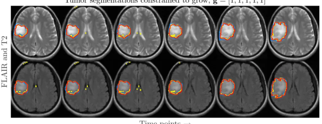
Tumor segmentations constrained to grow, g = [1,1,1,1,1]

Time points → F L A IR an d T 2

Fig. 2. FLAIR and T2 images for one patient (same patient as in the rightmost plot of Fig. 1) for six time points, annotated with EM segmentations (yellow ), NPGM segmentations with a strict growth constraint along time (red ) and ground truth (blue).

[0, 1]. This experiment is of clinical relevance: tumors tend to shrink temporarily after therapy and tumor regrowth needs to be detected as soon as possible. For each dataset, the algorithm will estimate confidence measures in g0 and g1. We obtain probabilities for both tumor growth patterns by normalising these confidence measures: [pg0, pg1] = [σg0, σg1]/(σg0+ σg1).

Figure 3 illustrates the amount of correctly classified tumor growth patterns. Of 168 datasets, 128 datasets were correctly classified, 35 datasets were falsely es-timated to grow after the second time point (false positives) and only 5 datasets were falsely estimated to keep shrinking after the second time point (false neg-atives). To the right in Fig. 3, one can see that the accuracy of tumor regrowth detection is highly related to the relative increase in tumor volume between the last time points. As expected, the difference in the tumor growth pattern probabilities (|pg1− pg0|) tends to be lower for misclassified tumor growth

pat-terns. Note that our classification detects either shrinkage or growth. In other words, it does not account for cases of ‘stable disease’, where the tumor is neither shrinking nor growing. This injects noise in our classification model, which gives rise to misclassifications. Figure 4 illustrates the segmentation of a rearranged dataset with a shrinking tumor that starts growing from the second time point on, together with tumor volumetry of T1, T1c, T2 and FLAIR.

Volumetric difference (%) -100 -50 0 50 100 150 P ro b ab il is ti c d iff er en ce (% ) 0 5 10 15 20 25 30 35 40 45 Volumetric difference 0 0.2 0.4 0.6 -1 Probabilistic difference 0 1 2 3 0.5 0 1 4 Accuracy: 0.7560 FN: 5, TN: 49 FP: 35, TP: 79 0.0530 ± 0.0646 0.2485 ± 0.5511 0.0898 ± 0.0852 _{-0.1068 ± 0.0861}

Fig. 3. Distribution of correctly (◦) and incorrectly (×) classified tumor growth

pat-terns as a function of the difference in the growth pattern probabilities (|pg1−pg0|) and

as a function of the relative increase in tumor volumes between the last time points.

4

Conclusion

In this study, we present a nonparametric model to segment brain tumors and to estimate the occurrence of tumor growth and/or shrinkage along time. We show the advantage of including longitudinal information in order to acquire more accurate tumor segmentations and volumetry. Furthermore, we adopt a fast and practical solution for the estimation of the spatial regularisation parameter

Tumor segmentations constrained to grow, g = [0,1] ← T im e p oi n ts

T1, T1c T2 and FLAIR Time points

1> 2< 3 4.5 5 5.5 6 6.5 7 7.5 8 Tumor volume in 2D annotated slices (cm3₎ T2 growth Flair growth T2 Ground Truth Flair Ground Truth

Time points 1> 2< 3 0 10 20 30 40 50 60 70 80 90 100 3D Tumor volume (cm3₎ T1 T1c T2 Flair

Fig. 4. Dataset depicting tumor regrowth occurring at the second time point, anno-tated with EM segmentations (yellow ), NPGM segmentations with g = [0, 1] (red ) and ground truth (blue). Volumes are given within the 2D ground truth annotated slices (in the middle) and for the entire 3D volumes (to the right ).

in the CRF energy function. Our model was extended to include probabilistic formulations for tumor regrowth after therapy, and it was shown to succeed in accurately estimating the occurrence of tumor regrowth.

References

1. Menze, B. H., Jakab, A., Bauer, S., et al.: The Multimodal Brain Tumor Image Segmentation Benchmark (BRATS). IEEE Trans. Med. Imag (2014)

2. Bauer, S., et al.: Integrated spatio-temporal segmentation of longitudinal brain tu-mor imaging studies. Proc MICCAI-MCV (2013)

3. Tarabalka, Y., et al.: Spatio-temporal video segmentation with shape growth or shrinkage constraint. IEEE Trans. Image Process. 23(9), 3829–3840 (2014) 4. Angelini, E. D., Clatz, O., Mandonnet, E., et al.: Glioma dynamics and

computa-tional models: a review. Current Medical Imaging Reviews 3, 262–276 (2007) 5. Gooya, A., et al.: Joint segmentation and deformable registration of brain scans

guided by a tumor growth model. Proc MICCAI (2), 532–540 (2011)

6. Boykov, Y., Kolmogorov, V.: An experimental comparison of min-cut/max- flow algorithms for energy minimisation in vision. IEEE Trans. Pattern Anal. Mach. Intell. 26(9), 1124–1137 (2004)

7. Candemir, S., Akgl, Y. S.: Adaptive parameter for graph cut segmentation. Lecture Notes in Computer Science 6111(1), 117–126 (2010)

8. Kohli, P., Torr, P.H.S.: Measuring uncertainty in graph cut solutions. Computer Vision and Image Understanding 112, 30–38 (2008)

9. Menze, B. H., Van Leemput, K., Lashkari, D., et al.: A generative model for brain tumor segmentation in multi-modal images. Proc MICCAI 13(2), 151–159 (2010)