HAL Id: hal-02372595
https://hal.archives-ouvertes.fr/hal-02372595
Submitted on 17 Dec 2020
HAL is a multi-disciplinary open access
archive for the deposit and dissemination of sci-entific research documents, whether they are pub-lished or not. The documents may come from teaching and research institutions in France or abroad, or from public or private research centers.
L’archive ouverte pluridisciplinaire HAL, est destinée au dépôt et à la diffusion de documents scientifiques de niveau recherche, publiés ou non, émanant des établissements d’enseignement et de recherche français ou étrangers, des laboratoires publics ou privés.
(CFEPS)-High-latitude Component
Jean-Marc Petit, J.J. Kavelaars, B.J. Gladman, R.Lynne Jones, J.W. Parker,
A. Bieryla, C. van Laerhoven, R.E. Pike, Phil D. Nicholson, M.L.N. Ashby, et
al.
To cite this version:
Jean-Marc Petit, J.J. Kavelaars, B.J. Gladman, R.Lynne Jones, J.W. Parker, et al.. The Canada– France Ecliptic Plane Survey (CFEPS)-High-latitude Component. Astronomical Journal, American Astronomical Society, 2017, 153 (5), pp.236. �10.3847/1538-3881/aa6aa5�. �hal-02372595�
arXiv:1608.02873v1 [astro-ph.EP] 9 Aug 2016
Pike , P. Nicholson , A. Bieryla , M.L.N. Ashby , S.M. Lawler
ABSTRACT
4
5 We report the orbital distribution of the Trans-Neptunian objects (TNOs) discovered
dur-ing the High Ecliptic Latitude (HiLat) extension of the Canada-France Ecliptic Plane Survey (CFEPS), conducted from June 2006 to July 2009. The HiLat component was designed to address one of the shortcomings of ecliptic surveys (like CFEPS), their lack of sensitivity to high-inclination objects. We searched 701 deg2of sky ranging from 12◦to 85◦ecliptic latitude
and discovered 24 TNOs, with inclinations between 15◦ to 104◦. This survey places a very
strong constraint on the inclination distribution of the hot component of the classical Kuiper Belt, ruling out any possibility of a large intrinsic fraction of highly inclined orbits. Using the parameterization of Brown (2001), the HiLat sample combined with CFEPS imposes a width 14◦ ≤σ ≤ 15.5◦, with a best match forσ = 14.5◦. HiLat discovered the first retrograde TNO,
2008 KV42, with an almost polar orbit with inclination 104◦, and (418993),a scattering object
with perihelion in the region of Saturn’s influence, witha ∼ 400 AU and i = 68◦.
Subject headings: Kuiper Belt, surveys
6
1. Introduction
7
The Kuiper Belt is widely thought of as a left-over flattened disk of planetesimals extending from
8
∼30 to a thousand AU from the Sun. Several Kuiper Belt surveys broke ground by investigating the gross
9
a
Institut UTINAM, CNRS-UMR 6213, Observatoire de Besanc¸on, BP 1615, 25010 Besanc¸on Cedex, France b
Department of Physics and Astronomy, 6224 Agricultural Road, University of British Columbia, Vancouver, BC, Canada c
Herzberg Institute of Astrophysics, National Research Council of Canada, Victoria, BC V9E 2E7, Canada d
Planetary Science Directorate, Southwest Research Institute, 1050 Walnut Street, Suite 300, Boulder, CO 80302, USA eDepartment of Planetary Sciences, University of Arizona, 1629 E. University Blvd, Tucson, AZ, 85721-0092, USA
f
Department of Physics and Astronomy, University of Victoria, Victoria, BC, Canada gCornell University, Space Sciences Building, Ithaca, New York 14853, USA h
Harvard-Smithsonian Center for Astrophysics, 60 Garden Street, Cambridge, MA 02138, USA i
properties of the TNO diameter and orbital distributions via large samples (Jewitt et al. 1996; Gladman et al.
10
2001; Millis et al. 2002; Trujillo et al. 2001). It is now obvious that this region must have been heavily
11
perturbed late in the process of giant planet formation. The Kuiper Belt’s small mass and the existence of
12
many objects with large orbital inclinations (i up to 50◦) indicate that a process either emptied most of the
13
mass out of the primordial Kuiper Belt or, more dramatically, that the Kuiper Belt was transported to its
14
current location during planetary migration. Recent models suggest stellar encounters (e.g., Levison et al.
15
(2010); Brasser et al. (2012)) or the existence of a 9th planet (Batygin & Brown 2016) may play an important
16
role in shaping the outer solar system.
17
The dynamical structure of the Kuiper Belt is much more complex than anticipated by the
commu-18
nity. Surveys with known high-precision detection efficiencies and which track essentially all their
ob-19
jects, to avoid ephemeris bias (Kavelaars et al. 2008; Jones et al. 2010), are needed to disentangle these
20
details and the cosmogonic information they provide. The Canada-France ecliptic plane survey (CFEPS)1
21
(Jones et al. 2006; Kavelaars et al. 2009; Petit et al. 2011, P1 hereafter), was a fully characterized2 survey
22
that tracked more than 80% of its discoveries to orbit classification3. Although discovering and tracking
23
only 169 TNOs, this survey produced solid science contributions to Kuiper Belt science (P1; Jones et al.
24
2006; Kavelaars et al. 2009; Gladman et al. 2012). Without this accurate calibration and extensive tracking,
25
it is risky to perform quantitative interpretation of the orbital distribution of the 800 multi-opposition TNOs
26
in MPC database with unknown detection and tracking biases (Jones et al. 2010).
27
The inclination distribution of the ‘main’ Kuiper Belt is now recognized as bimodal (Brown 2001;
28
Kavelaars et al. 2008), with a ‘cold’ component of objects with inclination width around 3◦ and a ‘hot’
29
component with a very broad inclination distribution, much like the disk/halo structure of the galaxy. This
30
discovery came at the same time as the realization that the cold component appears to have a different colour
31
distribution than the hot component (Doressoundiram et al. 2002; Tegler et al. 2003; Fraser & Brown 2012;
32
Peixinho et al. 2015). The orbital distribution of these high-inclination objects has a huge lever arm on
mod-33
els of outer Solar System formation and evolution, which include ideas like passing stars (Ida et al. 2000;
34
Kenyon & Bromley 2004; Morbidelli & Levison 2004; Kaib et al. 2011) that predict mean inclinations
in-35
creasing with semimajor axis, rogue planets (Gladman & Chan 2006) that predict inclination decreasing
36
with semimajor axis or transplanting almost all TNOs to their current locations during a large-scale
reorga-37
nization of the planetary system (Thommes et al. 1999; Levison et al. 2008; Nesvorny 2015).
38
For both components the distribution of orbital inclination can be modelled asP (i) ∝ sin (i) exp (−i2/2σ2)
39
(Brown 2001). The distribution of the hot component appears to have a Gaussian width σ of at least
40
15◦ (P1; Brown 2001; Kavelaars et al. 2009; Gulbis et al. 2010), but constraining the largest inclinations
41
is difficult because detection biases in ecliptic surveys strongly disfavour their discovery. About two dozen
42
1
http://www.cfeps.net
2A survey is characterized when all detection circumstances are known: telescope pointings, efficiency of detection w.r.t. mag-nitude and apparent motion, ..., so that one can simulate the survey. It is fully characterized if tracking has no orbital bias. An object is characterized when its detection efficiency is large enough that it is accurately determined (Petit et al. 2004)
3
Kuiper Belt objects with large inclinations spend the majority of their time at high ecliptic latitudes
46
(Fig. 1) and are poorly represented in the ecliptic surveys (including the main component of CFEPS). Even
47
more dramatically, it has become clear that the size distribution of the high inclination component is flatter
48
(number of objects increases slower when size decreases) than the ecliptic component (P1; Levison & Stern
49
2001; Bernstein et al. 2004; Fraser et al. 2014). So deeper surveys concentrating on the ecliptic will be
50
increasingly dominated by low inclination objects.
51
The situation at the end of 2006 was that a large fraction of the sky within a few degrees of the ecliptic
52
had been covered by a few large surveys, with magnitude limits in the range ofmR=20–23. Being insensitive
53
to high inclination objects (Fig. 2), ecliptic surveys have poor sensitivity to the width of the hot population.
54
Thanks to two deep blocks of 11 deg2(one at 10◦and another at 20◦ecliptic latitude) the CFEPS efficiency
55
decreases less than most other ecliptic surveys towards higher ecliptic latitudes. Still, although CFEPS
56
preferes a hot population inclination width σ of 16◦, it could not reject a width of 25◦. Actually what
57
limits the value ofσ is the relative decrease of the number of low and intermediate inclination objects when
58
increasingσ. Using the converted Palomar Schmidt, Trujillo & Brown (2003) had examined the majority of
59
the northern sky to a depth ofmR ∼ 20.5 (limit for median observing conditions), discovering several of
60
the largest known objects; several of these large-inclination objects (like Eris) were close to the depth and
61
motion limits of that survey due to their great distances. The ESSENCE Supernova Survey (Becker et al.
62
2008) announced the detection of 14 TNOs found in images covering ∼11 deg2 tor′ ∼23.7 in the ecliptic
63
latitude range -21◦ to -5◦; this work also showed that once outside of the ecliptic core, the sky density is
64
consistent with even a uniform distribution in latitude. Such a distribution would not be rejected by any
65
characterized surveys known at the time. We decided to perform a deep survey to magnitudemR ∼23.5–
66
24.0 at high (> 15◦) ecliptic latitudes, called HiLat, to probe the hot component of the Kuiper Belt at sizes
67
smaller than achieved by the Palomar wide area survey (Trujillo & Brown 2003) and SDSS. Although HiLat
68
is insensitive to objects with inclinations below 10◦ecliptic latitude (Fig. 2), it complements existing surveys
69
because its design makes it very sensitive to objects having inclinations beyond 20◦–30◦(Fig. 2).
70
This manuscript describes the observations carried out during the six years of the project and provides
71
our complete catalog (the HiLat release) of off-ecliptic detections and characterizations along with fully
72
linked high-quality orbits. In summary, the ‘products’ of the HiLat survey consist of four items:
73
1. A list of detected HiLat TNOs, associated with the sky location of discovery,
74
2. a characterization of each survey discovery observation (detection efficiency as a function of
magni-75
tude, motin on sky; rate range searched; pointing of observations; etc.),
76
3. a Survey Simulator that takes a proposed Kuiper Belt model, exposes it to the known detection biases
77
of the HiLat blocks and produces simulated detections to be compared with the real detections, and
78
4. the updated CFEPS model populations accounting for the HiLat detections.
−60
−40
−20
0
20
40
60
Latitude
0.00
0.01
0.02
0.03
0.04
0.05
0.06
Fra
cti
on
of
tim
e
Typical
Ecliptic Sur ey
Sample high ecliptic
latitude obser ation patch
50 degree inclination
Fig. 1.— Fraction of time spent at each ecliptic latitude for a sample object with an orbital inclination of 50 degrees. Previous surveys have mostly concentrated on low ecliptic latitudes where their sensitivity to high inclinations objects is comparatively low (central grey region). A survey concentrating on the area between 40–50◦latitude (like parts of HiLat, see Table 1 and Fig. 3, left grey region), where high inclination objects
0 10 20 30 40 50 60 70 80 90
Inclination (deg)
0.0 0.2 0.4 0.6 0.8 1.0A
rb
it
ra
ry
d
et
ec
ti
on
e
ff
ic
ie
nc
y
CFEPS and HiLat
relative survey efficiency
Fig. 2.— An illustration of the contrasting detection efficiencies of CFEPS (solid line) and HiLat (dashed line) as a function of ecliptic inclination, given their actual pointing histories. The orbital distribution model used here is the one derived from CFEPS, except for the inclination which was drawn uniformly between 0–90◦. The scaling of each histogram is arbitrary, what matters here is the relative efficiency of a given
2. Observations and Initial Reductions
80
The discovery component of the HiLat project imaged ∼700 square degrees of sky, all of which was
81
at ecliptic latitude larger than 12◦, extending almost to the North ecliptic pole (85◦, Fig. 3). Discovery
82
observations, comprising a triplet of images 1 hour apart each on the date listed in Table 1, and a nailing
83
observation, a single image acquired a few nights away from the discovery triplet, were all acquired using
84
the Canada-France-Hawaii Telescope (CFHT) MegaPrime camera which delivered discovery image quality
85
(FWHM) of 0.7–0.9 arc-seconds in queue-mode operations. The observations occured in blocks of 11 to
86
32 contiguous fields, cycling three times between the fields. The number of fields observed in a series was
87
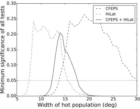
chosen such as to have ∼1 hour between two consecutive observations of the same field. When a block was
88
too large to be observed within one night, it was split into two sub-blocks observed during close-by nights,
89
with similar observing conditions. All discovery imaging data is publicly available from the Canadian
90
Astronomy Data Centre (CADC4).
91
The HiLat designation of a block was: a leading ‘HL’ followed by the year of observations (6 to
92
9) and then a letter representing the two week period of the year in which the search observations were
93
acquired (example: HL7j occured in the second half of May 2007), similar to CFEPS naming scheme.
94
Discovery observations occurred between June 2006 and June 2008 for the coverage below 60◦ ecliptic
95
latitude, followed by observations between 60◦ and 85◦ ecliptic latitude from May to July 2009. This last
96
part of the survey is simply named HL9 as it was acquired as 22 contiguous blocks over this time span.
97
The discovery fields were chosen in order to maximize our sensitivity to the latitude distribution of the
98
Kuiper Belt, in particular the high inclination TNOs. Observing at high ecliptic latitude ensured that we
99
observed only high-inclination TNOs, and greatly decreased the pressure for follow-up observations, as the
100
number of TNOs per unit area drops sharply away from the ecliptic. The ecliptic longitudes were chosen
101
to avoid the galactic plane, and maximize our chances to get discovery and tracking observations (due to
102
typical weather at time of opposition for the discovery field, observing request pressure on the telescope).
103
Each of the discovery blocks was searched for TNOs using our Moving Object Pipeline (MOP; see Petit et al.
104
2004). Table 1 provides a summary of the survey fields, imaging circumstances and detection thresholds.
105
Subsequent tracking, over the next 2 or more oppositions, occurred at a variety of facilities, including CFHT,
106
summarized in Table 2. The field sequencing and follow-up strategy of this survey are similar to those of
107
CFEPS (Allen et al. 2006; Kavelaars et al. 2009; Petit et al. 2011). Our discovery and tracking observations
108
were made using short exposures designed to maximize the efficiency of detection and tracking of the TNOs
109
in the field. These observations do not provide the high-precision flux measurements necessary for possible
110
taxonomic classification based on broadband colours of TNOs and we do not comment here on this aspect
111
of the HiLat sample.
112
4
Table 1. Summary of Field positions and Detections.
Block RA Dec Area Fill Detections Ecl. lat. Discovery limit Detection limits HRS deg deg2 Factor D T range (deg) date filter rAB rate (“/h) direction (deg)
HL6l 18:16 -06:49 15 0.80 0 0 11:50–20:50 2006-06-23 r.MP9601 22.37 0.5 to 6.1 -17.8 to 16.4 HL6r 22:37 +07:04 16 0.80 7 6 12:20–16:40 2006-09-18 r.MP9601 23.89 0.5 to 6.1 -43.6 to -8.2 HL7a 13:06 +55:00 32 0.90 0 0 49:40–60:00 2007-03-18 r.MP9601 23.58 0.5 to 5.7 6.6 to 47.8 HL7b 11:33 +37:30 32 0.88 0 0 27:00–35:40 2007-03-23 r.MP9601 22.89 0.5 to 5.4 -10.0 to 33.8 HL7c 11:33 +29:30 32 0.89 4 4 19:50–28:40 2007-03-21 r.MP9601 23.72 0.5 to 5.8 -3.1 to 36.3 HL7d 12:49 +57:00 32 0.84 0 0 49:30–59:50 2007-04-09 r.MP9601 23.28 0.5 to 4.6 -25.7 to 26.9 HL7e 13:23 +52:58 32 0.87 0 0 49:40–60:10 2007-04-22 r.MP9601 23.47 0.5 to 4.7 -25.2 to 27.0 HL7j 16:22 +12:53 32 0.90 5 5 22:50–40:20 2007-06-12 r.MP9601 23.49 0.5 to 5.6 -22.0 to 19.8 HL7l 17:47 +18:03 27 0.90 0 0 37:50–45:00 2007-06-12 r.MP9601 23.35 0.5 to 6.2 -10.1 to 22.1 HL7o 22:12 +22:02 32 0.90 0 0 20:30–39:40 2007-08-20 r.MP9601 22.74 0.5 to 6.3 -28.0 to 1.2 HL7p 22:06 +19:23 32 0.84 4 4 19:40–39:10 2007-09-06 r.MP9601 23.85 0.5 to 6.2 -41.3 to -7.3 HL7s 23:59 +27:54 31 0.98 0 0 19:30–37:00 2007-09-19 r.MP9601 23.38 0.5 to 6.3 -35.3 to -3.9 HL8a 09:24 +63:30 30 0.90 1 1 40:00–50:20 2008-01-08 r.MP9601 23.76 0.6 to 6.6 22.1 to 50.1 HL8b 09:52 +61:60 25 0.90 0 0 40:30–49:50 2008-01-09 r.MP9601 23.24 0.6 to 6.6 26.0 to 54.0 HL8h 16:32 +09:58 11 0.88 0 0 29:10–35:50 2008-05-05 r.MP9601 23.91 0.5 to 6.2 5.4 to 35.8 HL8i 16:21 +25:33 11 0.90 0 0 44:40–47:30 2008-05-09 r.MP9601 24.31 0.5 to 6.3 8.1 to 37.5 HL8k 17:35 +24:25 12 0.90 1 1 44:50–49:50 2008-05-11 r.MP9601 24.63 0.5 to 6.4 16.4 to 41.0 HL8l 17:36 +19:15 13 0.90 0 0 39:40–45:50 2008-05-13 r.MP9601 24.15 0.5 to 6.3 13.0 to 38.8 HL8m 16:58 +23:15 12 0.90 0 0 39:50–49:50 2008-05-30 r.MP9601 24.26 0.5 to 6.1 -7.9 to 26.1 HL8n 16:53 +22:33 11 0.89 1 1 39:40–50:30 2008-05-31 r.MP9601 24.80 0.5 to 6.1 -9.1 to 25.5 HL8o 16:48 +23:00 12 0.90 0 0 39:30–50:20 2008-06-07 r.MP9601 24.26 0.5 to 5.8 -17.7 to 21.1 HL9 18:45 +55:08 219 0.92 1 1 59:30–85:20 2009-06-16 r.MP9601 24.28 0.5 to 20.0 -20.0 to 90.0 Grand Total 701 24 21
Note. — RA/Dec is the approximate center of the field. Fill Factor is the fraction of the rectangle Area covered by the mosaic and useful for TNO searching. D is the number of TNOs detected in the block, T is the number of them that have been tracked to dynamical classification. Only one HL6r detection with apparent magnitude beyond the characterization limit, was not tracked to a high-quality orbit. The limiting magnitude of the survey, rAB,
is in the SDSS photometric system and corresponding to a 40% efficiency of detection. Detection limits give the limits on the sky motion in rate (“/hr) and direction (“zero degrees” is due West, and positive to the North).
Table 2. Follow-up/Tracking Observations.
UT Date Telescope Obs. UT Date Telescope Obs.
2006 Nov 22 WIYN 3.5-m 8 2008 Aug 31 CFHT 3.5-m 6
2007 Apr 13 CFHT 3.5-m 6 2008 Oct 22 WIYN 3.5-m 9
2007 May 14 Hale 5-m 13 2008 Dec 15 Hale 5-m 13
2007 May 14 KPNO 2.1-m 7 2008 Dec 20 WIYN 3.5-m 17
2007 Jul 26 CFHT 3.5-m 3 2009 Jan 26 CFHT 3.5-m 7
2007 Sep 10 WIYN 3.5-m 8 2009 Mar 25 Subaru 8.2-m 2
2007 Sep 13 CFHT 3.5-m 20 2009 Apr 22 Subaru 8.2-m 5
2007 Sep 15 Hale 5-m 25 2009 Jun 19 WIYN 3.5-m 30
2007 Oct 07 CFHT 3.5-m 6 2009 Jul 18 CFHT 3.5-m 5
2007 Nov 08 WIYN 3.5-m 17 2009 Jul 23 Hale 5-m 31
2008 Mar 04 CFHT 3.5-m 12 2009 Aug 17 Hale 5-m 6
2008 Mar 08 CFHT 3.5-m 3 2009 Aug 18 CFHT 3.5-m 6
2008 Apr 04 CFHT 3.5-m 10 2009 Sep 12 CFHT 3.5-m 4
2008 May 02 WIYN 3.5-m 21 2009 Sep 13 CFHT 3.5-m 27
2008 May 05 CFHT 3.5-m 21 2009 Oct 12 CFHT 3.5-m 8
2008 May 28 CFHT 3.5-m 14 2009 Nov 15 CFHT 3.5-m 4
2008 Jun 01 CFHT 3.5-m 3 2010 Jan 20 CFHT 3.5-m 3
2008 Jun 07 CTIO 4-m 20 2010 Mar 19 Hale 5-m 12
2008 Jun 22 MMT 6.5-m 4 2011 May 02 Magellan 6.5-m 8
2008 Jul 07 Gemini South 8.1-m 5 2013 Feb 06(a) Gemini North 8.1-m 42
2008 Aug 05 CFHT 3.5-m 24 2013 Jul 05 NOT 2.5-m 13
2008 Aug 30 CFHT 3.5-m 52 2013 AUg 05(a) Gemini North 8.1-m 32
Note. — All observations not part of the HiLat discovery survey are reported here. UT Date is the start of the observing run; Obs. is the number of astrometric measures reported from the observing run. Runs with low numbers of astrometric measures were either wiped out by poor weather, or not meant for HiLat object follow-up originally. (a) This is the date of the first observation; targets were observed twice a month throughout the semester.
0
50
100
150
200
250
300
350
RA (deg)
)20
0
20
40
60
80
DE
C (
de
g)
HL6
HL6r
HL7a
HL7b
HL7c
HL7d
HL7e
HL7j
HL7
HL7o
HL7p
HL7s
HL8a
HL8b
HL8h
HL8i
HL8k
HL8
HL8m,n,o
HL9
Nept(ne
Fig. 3.— Geometry of the HiLat discovery-blocks. The RA and Dec grid is indicated with dotted lines. The solid curves show constant ecliptic latitudes of 0◦, 30◦, 60◦, 80◦, from bottom to top. The blue rectangles
mostly along the eclitpic indicate CFEPS pointings, the cyan rectangles indicate the HiLat survey pointings. The red diamond indicates the position of Neptune on 2016-07-31.
3. Sample Characterization
113
As is now the norm (Trujillo & Jewitt 1998; Jewitt et al. 1998; Gladman et al. 1998; Trujillo et al.
114
2000; Gladman et al. 2001; Petit et al. 2006; Kavelaars et al. 2009; Petit et al. 2011), we characterized the
115
magnitude-dependent detection probability of each discovery block by inserting artificial sources in the
im-116
ages. We performed differential aperture photometry for each of our detected objects observed on
photomet-117
ric nights. Our photometry is reported in the Sloan system (Fukugita et al. 1996) with the calibrations
con-118
tained in the header of each image as provided by the ELIXIR processing software (Magnier & Cuillandre
119
2004). It can be found in Tables 3 and 4. All HiLat discovery observations that detected TNOs were acquired
120
in photometric conditions in a relatively narrow range of seeing conditions due to queue-mode acquisition.
121
Those real objects in each block that have a magnitude brighter than that block’s 40% detection
prob-122
ability are considered to be part of the HiLat characterized sample. Because detection efficiencies below
123
∼40% determined by human operators and our software diverge (Petit et al. 2004), and since
characteriza-124
tion is critical to our goals, we are unable to utilize the sample faint-ward of the measured 40% detection
125
efficiency level for quantitative analysis (although we report these discoveries, the majority of which were
126
tracked to precise orbits). The characterized HiLat sample consists of 21 objects of the 24 discovered
127
(Table 3). The magnitude distribution of objects detected brighter than our cutoff is consistent with the
128
shape of the TNO luminosity function (Petit et al. 2008) and the typical decay in detection efficiency due to
129
gradually increasing stellar confusion and the rapid fall-off at the SNR limit.
130
4. Tracking
131
For typical (i.e., low ecliptic latitude) surveys to depthr′ ∼23.5–24, the observing load of tracking
132
observations to secure the objects and determine their orbits represents many times the time spent for
discov-133
ery. In such a case, a ∼700 square degree survey with fully tracked objects would be prohibitive. However,
134
because HiLat covers very high ecliptic latitudes, the number of object per square degree at our limiting
135
magnitude goes down dramatically beyond 30–35◦ and we detected only 24 objects (21 characterized).
136
Hence the tracking observing load was much lower than for an ecliptic survey and
137
All of the 21 characterized and 2 of the 3 non-characterized objects were followed for at least 3
op-138
positions. Objects that still had uncertain dynamical classifications were then followed up to 7 oppositions,
139
mostly for resonant or near-resonant objects. The global release of the complete observing record for all
140
HiLat objects is available from the MPC (Petit et al. 2015) and the entire astrometric data for the HiLat
141
objects can be found on the Besanc¸on TNO database5. The correspondence between HiLat internal
designa-142
tions and MPC designations can be determined using Tables 3 and 4 or from the Besanc¸on TNO database.
143
All characterized and tracked objects are prefixed by HL and are used with the survey simulator for our
144
modelling below.
145
Table 3. Characterized Object Classification.
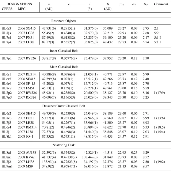
DESIGNATIONS a e i R mr σr Hr Comment CFEPS MPC (AU) (◦) (AU)
Resonant Objects
HL6r3 2006 SG415 47.931(6) 0.2915(1) 31.376(0) 35.009 23.27 0.03 7.75 2:1 HL7j3 2007 LG38 55.45(2) 0.4340(3) 32.579(0) 32.219 22.93 0.09 7.68 5:2 HL7c1 2007 FN51 87.49(3) 0.6188(2) 23.237(0) 39.100 23.20 0.06 7.17 5:1 I HL7j4 2007 LF38 87.57(3) 0.5552(2) 35.825(0) 48.432 22.53 0.09 5.54 5:1 I
Inner Classical Belt
HL7p1 2007 RY326 38.817(9) 0.06776(9) 25.479(0) 37.952 23.20 0.12 7.30 Main Classical Belt
HL6r1 2007 RL314 40.386(8) 0.0386(4) 21.057(1) 40.771 22.97 0.07 6.79 HL6r5 2006 SE415 42.599(8) 0.027(1) 18.517(1) 42.266 23.73 0.12 7.40 HL6r6 2006 SF415 43.20(2) 0.077(1) 15.712(0) 40.713 23.87 0.09 7.70 HL7c2 2007 FM51 45.53(1) 0.159(1) 29.221(1) 42.561 23.00 0.15 6.59 HL7p2 2007 RW326 45.92(1) 0.2355(2) 20.500(0) 35.127 23.70 0.10 8.16 I (17:9) HL7p3 2007 RX326 46.096(7) 0.1565(3) 25.029(0) 39.343 23.30 0.30 7.25
Detached/Outer Classical Belt
HL6r2 2006 SH415 49.759(9) 0.2539(3) 25.048(0) 38.189 23.60 0.06 7.71 HL7c3 2007 FO51 50.37(3) 0.2873(6) 27.946(0) 37.560 22.87 0.19 6.99 I (13:6) HL7j5 2007 LE38 54.05(1) 0.2267(1) 35.966(1) 41.800 23.27 0.07 6.93 HL6r4 2007 RM314 70.81(2) 0.4846(2) 20.884(0) 42.622 22.70 0.17 6.33 I (18:5) HL7j1 2007 LJ38 72.37(3) 0.4698(3) 31.540(0) 38.848 23.07 0.19 7.03 I (15:4) HL8k1 2008 JO41 87.35(2) 0.5431(1) 48.815(0) 44.453 24.57 0.12 7.91 Scattering Disk HL8a1 2008 AU138 32.392(3) 0.3745(2) 42.826(1) 44.518 22.93 0.23 6.29 HL8n1 2008 KV42 41.532(4) 0.49138(7) 103.447(0) 31.849 23.73 0.03 8.52 HL7j2 2007 LH38 133.93(4) 0.72523(8) 34.197(0) 37.376 23.37 0.03 7.50 I (19:2) HL9m1 2009 MS9 348.9(2) 0.96847(1) 68.016(0) 12.872 21.13 0.09 9.57
Note. — a: semimajor-axis (AU); e: eccentricity; i: inclination (degrees); R: distance to the Sun at discovery time (AU); mr: apparent magnitude of the object in MegaPrime r′filter; σr: uncertainty on the magnitude in that filter; Hris
the absolute magnitude in r band, given the distance at discovery; In Comment column, M:N: object in the M:N resonance; I: indicates that the orbit classification is insecure (see Gladman et al. (2008) for an explanation of the exact meaning); (M:N): the insecure object may be in the M:N resonance. For the orbital elements the number in “()” gives the uncertainty on the last digit.
Table 4. Non Characterized Object Classification.
DESIGNATIONS a e i R mr σr Hr Comment
CFEPS MPC AU ◦ AU
Resonant Objects
uHL7c4 2007 FP51 44.760(6) 0.2017(1) 25.606(0) 36.688 23.80 0.20 8.02 20:11 I Detached Classical Belt
uHL7p4 2007 RZ326 52.676(8) 0.3465(1) 37.268(0) 38.300 23.93 0.09 7.98 Non classified objects
uHL6r7 2006 SN415 — — — 38(7) 24.50 0.25 8.65
are as small as a few tenths of an arcsecond for several objects, others have uncertainties up to of order
149
10 arcseconds. Our protocol was to pursue tracking observations until the semimajor axis uncertainty was
150
< 0.1%; in Tables 3 and 4, orbital elements are shown to the precision with which they are known, with
151
typical fractional accuracies on the order of a few10−4. In the cases of resonant objects even this precision
152
may not be enough to precisely determine the amplitude of the resonant argument, or even securely classify
153
them as resonant. Thanks to our intensive tracking effort, dynamical classification is possible for 100% of
154
the characterized sample.
155
4.1. Orbit classification
156
We follow the dynamical classification scheme of Gladman et al. (2008), which was also used to
de-157
termine the classification of the CFEPS sample. In this scheme, the Kuiper Belt is divided into three broad
158
orbital classes based on orbital elements and dynamical behavior. We first check if the object is resonant
159
(currently in MMR with Neptune or Uranus), then see if it is currently scattering (practically defined as a
160
variation of semimajor axis of more than 1.5 AU in a forward time integration over 10 Myr). If not, it is
161
a classical or detached object: Inner classical if semimajor axis is interior to the MMR 3:2 with Neptune;
162
main classical if semimajor axis between the 3:2 and 2:1 MMR; outer classical if semimajor axis beyond
163
the 2:1 MMR ande < 0.24; detached if semimajor axis beyond the 2:1 MMR and e > 0.24).
164
Using this classification procedure, 7 of our 21 characterized objects remain insecure, as defined in
165
Gladman et al. (2008), due to their proximity to a (high-order) resonance border where the remaining
astro-166
metric uncertainty makes it unclear if the object is actually resonant. We list these “insecure” objects in the
167
category shown by the majority of the clones (Gladman et al. 2008) and give the nearby resonance in the
168
comment column. Table 3 gives the classification of all characterized objects. None of these objects had
169
archival observations before our discovery. Table 4 gives the classification of the tracked objects below the
170
40% detection efficiency threshold, hence deemed un-characterized and not used in our Survey Simulator
171
comparisons.
172
The apparent motion of TNOs in our opposition discovery fields is approximatelyθ(”/hr) ≃ (147 AU)/R,
173
whereR is the heliocentric distance in AU. With a typical seeing of 0.7–0.9 arcsecond and a time base of
174
70–90 minutes between first and third frames, we were sensitive to objects as distant asR ≃ 125 AU,
pro-175
vided they are brighter than our magnitude limit. Despite this sensitivity to large distances, the most distant
176
object discovered in HiLat lies at 48.4 AU from the Sun (HL7j4, an insecure resonant object in the 5:1 MMR
177
with Neptune (Pike et al. 2015)).
5. Results
179
CFEPS data presented in P1 were modelled independently for the inner, main, outer/detached classical,
180
the scattering and various resonant populations by P1 and Gladman et al. (2012). The model for the main
181
classical belt is refered as the L7 model hereafter. According to P1, the cold component may very well exist
182
only in the main classical belt. The hot component, on the contrary, permeates the whole belt, from the inner
183
classical, to the main classical, to the outer/detached belt and all the resonances. The cold component was
184
well constrained by the Ecliptic component of the survey.
185
HiLat was designed to have maximum sensitivity to high-inclination objects (Fig. 2), and thus places
186
strong constraints on the distribution of high-inclination objects, i.e., the hot population. The goal is thus to
187
improve the L7 model.
188
5.1. Main Classical belt and L7 model
189
Our aim is to create a model that is compatible with both the CFEPS and HiLat detections. We are able
190
to account for HiLat detections by slightly changing some parameters of the L7 orbital model, affecting only
191
regions of phase space not well constrainted by CFEPS detections. Here we concentrate on the model for
192
the main classical belt, because this dynamical class alone constitutes nearly a third of the full HiLat sample.
193
With the parameterization of L7 model, HiLat is sensitive almost exclusively to the hot component. Hence
194
this is the part of the model that will be modified in the following. However, in what follows, we always run
195
the full L7 model, including all components: kernel, stirred and hot components.
196
5.1.1. Orbital model
197
To estimate the quality of a model, we compare the survey detected sample to the sample returned by
198
passing our intrinsic model through a survey simulator (see Jones et al. 2006, for details). Acceptance of a
199
model is based on the Anderson-Darling statistic for each ofa, e, i, q [perihelion distance], R and r′and its
200
level of significances (probability of the null hypothesis [the simulated and the observed samples are drawn
201
from the same underlying distribution] being correct), determined using a bootstrap method (Press et al.
202
1992).1−s gives the rejectability of that hypothesis. As for CFEPS, we reject a model when the rejectability
203
exceeds 95%. We determine the rejectability on the maximum of all 6 indicators we consider. When creating
204
the L7 model, P1 split the phase space into sub-regions (see Appendix A of P1) to help separate the hot and
205
cold components and account for the kernel and stirred components. HiLat detects almost exclusively the
206
hot component, and the sample size is small, thus we determine the significance examining the full orbital
207
phase space occupied by the main-belt.
208
Using the improved survey simulator (see Bannister et al. (2016a) for a description of the
improve-209
ments) against the CFEPS detections, the L7 model for the main classical belt retains the same level of
210
significance (∼20%) as with the previous survey simulator.
different filters, and accepts as input the colours of each object. Here, for compatibility with previous works,
215
we assumeg′−r′= 0.7 and g′−R= 0.8 (this assumption agrees with more recent results from OSSOS, the
216
Outer Solar System Origin Survey; Bannister et al. 2016a).
217
When the biased L7 model is tested agaijnst the HiLat detections, thei and q distributions of the hot
218
component are rejectable at> 95%. An important feature of the L7 model for the main classical belt is the q
219
distribution of the hot component (see Appendix A of P1), which is essentially uniform between two limits,
220
with rapid roll-over at both ends, with a width of 0.5 AU. The upper limit is poorly constrained by CFEPS.
221
To account for HiLat detections, we moved the upper roll-over of the hot-componentq distribution from 40
222
to 41 AU, still with a width of 0.5 AU. Because HiLat did not detect any main classical belt object with
223
q < 35 AU, we must impose a sharp cut-off on top of the i-dependent lower-limit of the hot-component q
224
distribution. The new parameterization is described in Appendix A. Using this slight tuning of the L7 model
225
continues to provide an acceptable match to the CFEPS detected sample, when considered independent of
226
the HiLat sample. Extending the q-distribution of the L7 model somewhat allows compatibility with the
227
HiLatq-distribution.
228
Thei-distribution of the HiLat main classical belt detected sample is incompatible with the hot
compo-229
nent of the L7 model. The CFEPS detected sample strongly rejects a hot population with a narrow inclination
230
width because that model does not yield the correct ratio between low inclination and high inclination as
231
compared to the detections in the CFEPS sample. The CFEPS sample rejects much larger inclination
distri-232
butions (σ ≥ 30◦; see Fig. 4, dashed line) only because of the relative lack of low inclination objects in these
233
distributions. The HiLat detected sample, on the contrary, rejects any model with too wide an inclination
234
distribution because this survey is very sensitive to the high inclination orbits. Even the inclination width
235
σ = 16◦ preferred by CFEPS has a long tail containing too many objects withi > 35◦ which would have
236
been detected by HiLat. But being completely insensitive to low inclination orbits (HiLat cannot detect any
237
of them), it can accept any values ofσ as long at they allow enough objects up to i ≃ 35◦. Thus HiLat
238
is consistent with all values ofσ from 7.5◦ to 15.5◦ (Fig. 4, dash-dotted line). Together, the two surveys
239
combine high CFEPS sensitivity at low inclinations and HiLat’s improved sensitivity at high inclinations.
240
The result is shown in Fig. 4. Because our model rejection threshold is set at 5% significance, this analysis
241
indicates that an acceptable value for each of CFEPS and HiLat separately and for their combination, is an
242
inclination widthσ in the range 14◦–15.5◦, where all three curves exceed the threshold.
243
Separately, CFEPS and HiLat favor different values for the width and only marginally agree at the
244
intersection (see Fig. 4). There is tension between the models allowed by the two data sets. This raises
245
doubts on the parameterization used here. Gulbis et al. (2010) introduced an inclination distribution given
246
by sin (i) times a Gaussian of width σ, centered on a value ic greater than 0◦ to fit what they called the
247
Scattered population (Appendix A). Pike et al. (2015) did the same to study the 5:1 MMR population. P1
248
mentioned the possibility to use a similar functional form to represent the Classical belt hot population
249
inclination distribution, but concluded that the fit was good enough with the usual distribution and that the
5
10
15
20
25
30
Width of hot population (deg)
0.00
0.05
0.10
0.15
0.20
0.25
0.30
Mi
nim
um
si
gn
ific
an
ce
of
al
l te
sts
CFEPS
HiLat
CFEPS + HiLat
Fig. 4.— Modelling the hot component of the main classical belt. Minimum level of significance of all 6 Anderson-Darling tests fora, e, i, q, R, and r′, as a function of the hot population inclination distribution
width, for CFEPS alone (dashed line), HiLat alone (dash-dotted line) and CFEPS and HiLat combined (solid line). The dotted line shows the 95% rejection threshold; any model with significance level below that line is rejected. The bumpiness of the curves is due to randomness in the survey simulator and in the bootstrapping of the Anderson-Darling statistics.
distribution functional form, with a width σ = 14.5◦. We note, however, that the functional form here,
254
while useful for discussion, is not a good description of the physical distribution of high-inclination TNOs.
255
5.1.2. Population estimates
256
Population estimates are dependent on the orbital model used to describe each TNO component, which
257
we are slightly modifying from P1. They also depend on the correct modelling of the survey operation
258
and detection efficiency. As explained in Bannister et al. (2016a), the survey simulator has been improved
259
to better represent the exact selection and rejection effects of objects based on measured magnitude rather
260
than intrinsic magnitude. This has the potential of substantially affecting the population estimates due to the
261
steep slopes of the absolute magnitude H distributions.
262
We follow the same procedure as in Kavelaars et al. (2009), Gladman et al. (2012), and P1. We run
263
our model, generating simulated objects, passing them through the survey simulator until we have detected
264
the same number of objects in the simulation as in the real survey(s). We record this number and repeat
265
the procedure 500 times. This gives us the distribution of likely population size. Table 5, columns A, gives
266
the population estimates, using our new model, toHg ≤8.0 to compare with P1. Compared to P1, we use
267
the newq-distribution and an i-distribution with width σh = 14.5◦. Our CFEPS estimates are statistically
268
undistinguishable from P1 estimates.
269
Although the various population estimates for a given component have overlapping error bars, HiLat
270
estimates population sizes at just a little over half those of CFEPS. This is also reflected in the larger than
ob-271
served fraction of objects detected from HiLat when running our model through the combined CFEPS +
Hi-272
Lat survey simulator; 12% of the simulated detections are from HiLat, while they represent only 6% of
273
the real sample. This larger fraction from HiLat means the model plus survey simulator are more efficient
274
at detecting objects in HiLat survey, hence needing a smaller underlying population to reach the required
275
number of detections. This may be due to our choice ofg′−r′color for TNOs, a necessary parameter when
276
combining surveys done in different band passes.
277
Up to now we used theg′−r′= 0.7 colour derived from CFEPS sample for all components. However,
278
the cold belt objects are redder than the hot ones (Doressoundiram et al. 2002; Tegler et al. 2003). If the hot
279
objects detected by HiLat are bluer thang′−r′ = 0.7, then the number of objects brighter than H
g = 8.0
280
needed to match the real detections is larger. According to Fraser (private communication, 2016), the cold
281
component has a typical colour0.8 < g′−r′< 1.1, while the hot component comprise mostly neutral objects
282
with0.4 < g′−r′ < 0.7, and a small fraction of objects as red as the cold component. Table 5, columns B,
283
gives the population estimates when usingg′−r′ = 0.45 for the hot component and g′−r′ = 0.95 for the
284
cold component. The three population estimates become more compatible with each other, and the fraction
285
of simulated detections from HiLat in CFEPS+HiLat simulations becomes 7%, similar to the real detected
Table 5. Model dependent population estimates forHg ≤8.0.
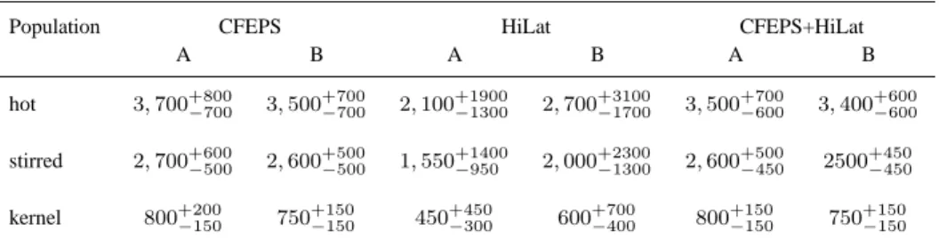
Population CFEPS HiLat CFEPS+HiLat
A B A B A B hot 3, 700+800−700 3, 500+700−700 2, 100−1300+1900 2, 700+3100−1700 3, 500+700−600 3, 400+600−600 stirred 2, 700+600−500 2, 600+500−500 1, 550−950+1400 2, 000+2300−1300 2, 600+500−450 2500+450−450 kernel 800+200 −150 750 +150 −150 450 +450 −300 600 +700 −400 800 +150 −150 750 +150 −150
Note. — Our model estimates are given for each sub-population within the Kuiper belt. The uncertainties reflect 95% confidence intervals for the model-dependent population estimate. Remember that the relative importance of each population will vary with the upper Hglimit. The A columns correspond to a uniform
colour g′− r′= 0.7, while B columns have g′− r′= 0.45 for the hot component and g′− r′= 0.95 for the
5.2. Other populations
289
The HiLat characterized sample included six outer classical or detached objects, roughly half as many
290
as were identified by CFEPS (P1 identified 13 non-scattering, non-resonant objects beyond 48 AU). P1
291
established that the outer-detached population can be interpreted as a smooth extention beyond the 2:1 MMR
292
of the hot main classical belt. We confirm this result with CFEPS+HiLat detection. We note however that
293
the HiLat sample alone allows inclination widths13◦ < σ < 30◦, possibly more excited than for the main
294
classical belt. The combined CFEPS+HiLat sample allows an inclination width12.5◦ < σ < 20◦. This is
295
in agreement with the outer-detached population being a smooth extension of the hot classical population.
296
We estimate the population beyond 48 AUN (Hg ≤8.0) = 9500+4500−3500, very similar to P1 estimate.
297
The HiLat characterized sample contains 4 resonant objects. One is in the 2:1 MMR and another one
298
in the 5:2 MMR with Neptune. These represent a small contribution to the known populations of these
reso-299
nances from characterized surveys like CFEPS. HiLat made an important contribution to our understanding
300
of the resonant population by discovering two objects in the 5:1 MMR (only 1 was known from CFEPS),
301
and another very close to the 5:1 MMR, HL8k1 = 2008 JO41at 87.356 AU; scientific interpretation of these
302
discoveries have been reported in Pike et al. (2015).
303
5.3. Exotic objects: 2008 KV42and (418993) 2009 MS9
304
Amongst its 21 characterized detections, HiLat discovered 2 extraordinary TNOs. Both are scattering
305
objects. The first one was discovered on May 31st, 2008 in a field at moderate ecliptic latitude (∼ 30◦). It
306
is HL8n1 = 2008 KV42, the first known retrograde TNO. Details about this object and what it tells us about
307
the origin and dynamical evolution of exotic scattering objects is developed in Gladman et al. (2009).
308
The second object is HL9m1 = (418993) 2009 MS9, discovered on the 26th of June 2009 at a distance
309
of 12.9 AU from the Sun and an ecliptic latitude of 71◦. It has a large (a ≃ 350 AU) and highly-inclined
310
(i ∼ 68◦) orbit (Fig. 5), which is also highly eccentric (e ≃ 0.968). Inbound at 13 AU at time of discovery,
311
the pericenter of this extreme orbit was ∼11 AU in February 2013, so (418993) is transiting the range of
he-312
liocentric distances where comets have been observed to become active (Meech & Svoren 2004). (418993)
313
thus may be the first observable object that has been in deep cold storage at hundreds of AU for of order
314
5,000 years. Under the hypothesis that this is a comet from a distant source (either the inner Oort Cloud, or
315
something else as yet unknown), it is also quite possible that (418993) has never been interior to Saturn’s
316
orbit (unlikely to be true for the known Centaurs, which often have their perihelia altered as they interact
317
with the giant planets).
318
A plausible scenario is that (418993) is a former Oort-cloud object that has had its orbit changed
100
200
300
400
500
600
semimajor
axis a(AU)
0
20
40
60
80
100
120
inc
lin
ati
on
i (
de
g)
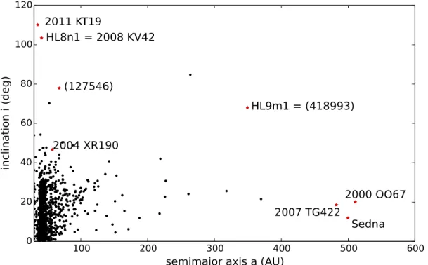
2004 XR190
2011 KT19
HL8n1 = 2008 KV42
(127546)
HL9m1 = (418993)
Sedna
2000 OO67
2007 TG422
Fig. 5.— Trans-Neptunian objects withq > 10 AU in orbital a/i space, in ASTORB database as of August 2nd, 2016. Since its discovery, 2009 MS9= (418993) stands out as unique (with othera > 300 AU TNOs
having inclinations in the ‘normal’ i < 20 deg range). 2008 KV42 is also very peculiar with a retrograde
after the development of a coma, but only after the comets have left the inner Solar System and are very dim
323
(Lamy et al. 2004). MS9 had the advantages that, at time of discovery, it was bright (r′∼22), inbound, and
324
had no obscuring coma. Assuming an albedo p=0.04 (common for comet nuclei, Lamy et al. 2004, but on
325
the lower end for TNOs), this object has a radius ≃20 km. Not only is (418993) unique dynamically, but if it
326
had become an active comet, it would have been the largest comet nucleus in recent times, after Hale-Bopp
327
(C/1995 O1; radius = 37 km; Lamy et al. 2004).
328
At its discovery distance of 13 AU, no coma has been detected in analysis of our deep August 2009
329
CFHT images, to a limit of 28 mag/arcsec2. Other shorter-period comets have been observed to start
330
cometary activity as far out as 12–14 AU from the Sun (1P/Halley at 14 AU and 2060 Chiron at 12 AU;
331
Meech & Svoren 2004). We observed (418993) at the Palomar 5m in August 2009, and determined that it
332
has a ∼ 0.4-mag lightcurve with a period of over either 6.5 (single peaked) or 13 hours (double peaked;
333
Fig. 6). Studying a possible cometary activity on this object requires determining the rotational phase to
334
remove this predictable brightness change. We obtained snapshot observations to monitor the cometary
ac-335
tivity from Aug. 2010 to Feb 2011 but detected none. From 2012 until end of 2014, many observations
336
of (418993) have been reported to MPC, around its perihelion passage, but none have reported detection of
337
cometary activity.
338
6. Summary and discussion
339
The HiLat survey was designed to address one of the shortcomings of CFEPS, its lack of sensitivity
340
to high-inclination objects. HiLat imaged about 700 sqr. deg. from 12◦to 85◦ecliptic latitude. The survey
341
was performed at CFHT in ther′ filter and achieved limiting magnitudes raging from r′ = 22.4 for the
342
shallowest field tor′ = 24.8 for the deepest field. Being at high ecliptic latitude, the survey detected only
343
24 objects, of which 21 are brighter than the characterization limit. Thanks to the small number of objects
344
and to our careful follow-up strategy, we tracked all characterized objects to precise orbit determination and
345
orbital classification.
346
HiLat detected 6 objects from the hot main classical belt. We confirm the global parameterization of
347
this component found by CFEPS. An important finding of CFEPS was that the q-distribution of the hot
348
classical component is essentially flat between 35 AU and 40 AU, with poor constraint on this upper limit.
349
The HiLat sample requires us to move the upper limit to 41 AU. Including the HiLat sample and survey in
350
the analysis, we decrease sightly the width of the inclination distribution of the hot component toσ = 14.5◦.
351
The high sensitivity of HiLat survey to TNOs on highly-inclined orbits permits formal rejection at high
352
confidence of ’wider’ orbital i-distributions for the hot classical belt, and to a lesser extent the detached
353
components. CFEPS survey already rejected ’narrower’i distributions. Having an i-distribution with little
354
contribution below about 10◦ and not extending much beyond 35◦–40◦ is difficult to achieve with a broad
1.6 1.7 1.8 1.9 JD-2455060
−0.3
−0.2
−0.1
0.0
0.1
0.2
rel
ati
ve
m
ag
s
r
-band g-band i-bandFig. 6.— Preliminary lightcurve from 18 and 19 August 2009 Palomar data. The magnitudes are relative to 8 field stars (with the mean removed). r-band (red diamond) and g-band (green triangle) photometry was obtained on both nights, while the i-band (blue star) was acquired only on the first night. The r- and g-band magnitudes have been arbitrarily adjusted to the same mean to show that there is no strong rotational colour dependence. The amplitude is ∼0.4 mag. Observations acquired on the 19 August 2009 have been arbitrarily shifted by 26 hours. This plot shows that the period is around 6.5 hour if single peaked or around if double peaked 13 hour. Although the single peaked solutino seems incompatible with this plot, the quality of the data does not allow to reject it firmly. Thus one needs a longer time span to really characterize the lightcurve.
cosmogonic implications that would need to be investigated.
359
The exotic higher-i objects like those found in HiLat (Fig. 5) do not fit into this picture; we will
360
call thesei ∼ 90◦ objects the ‘halo’ component. Due to our sensitivity to high inclinations, these do not
361
represent the tail of the 14.5◦ gaussian. Instead, these objects may point to a new source that feeds large-i
362
TNOs into the planetary system (Gladman et al. 2009). This may simultaneously be the source of the
Halley-363
Type comets (see Levison et al. 2006). Recently, Batygin & Brown (2016) pointed to (418993) as possible
364
evidence that this source might be related to an undiscovered planet in the distant solar system (a ∼ 500 au);
365
producinga < 50 objects like 2008 KV42requires pulling objects from such a large-a source down to such
366
small semimajor axes and is exceedingly difficult due to the high encounter speeds with Neptune and Uranus
367
(Gladman et al. 2009).
368
The OSSOS Survey (Bannister et al. 2016a,b) will allow a careful consideration of the details of the
369
i-distribution of the main hot component and the relative fraction of objects that must be in this halo
popula-370
tion. The use of our characterized Hilat survey (coupled to CFEPS and OSSOS) permits powerful constraints
371
to be placed on thea/q/i distribution generated by any proposed model of where these extreme objects are
372
coming from.
373
A. Appendix A
374
We here detail the minor tuning to the L7 algorithm used to generate the hot population of the main
375
classical belt, motivated by the HiLat sample’s greater sensitvity. The new algorithm becomes:
376
• a perihelion distanceq distribution that is mostly uniform between 35 and 41 AU, with soft shoulders
377
at both ends extending over ∼1 AU; the PDF is proportional to 1/([1 + exp ((35 − q)/0.5)][1 +
378
exp ((q − 41)/0.5)]); any object with q <35 AU is rejected;
379
• reject objects withq < 38 − 0.2i (deg) to account for weaker long-term stability of low-q orbits at
380
low inclination.
381
The inclination distribution for the hot component remains P (i) ∝ sin(i) exp (−i2/2σ2), but with σ =
382
14.5◦.
383
Acknowledgments: This work is based on observations obtained with MegaPrime/MegaCam, a joint project
384
of CFHT and CEA/DAPNIA, at the Canada-France-Hawaii Telescope (CFHT) which is operated by the
Na-385
tional Research Council (NRC) of Canada, the Institute National des Sciences de l’Universe of the Centre
386
National de la Recherche Scientifique (CNRS) of France, and the University of Hawaii. This research
387
was supported by funding from the Natural Sciences and Engineering Research Council of Canada, the
Canadian Foundation for Innovation, the National Research Council of Canada, and NASA Planetary
As-389
tronomy Program NNG04GI29G. This project could not have been a success without the dedicated staff of
390
the Canada-France-Hawaii telescope as well as the assistance of the skilled telescope operators at KPNO
391
and Mount Palomar. This work is based in part on data produced and hosted at the Canadian Astronomy
392
Data Centre.
393
Facilities: CFHT (MegaPrime), WIYN, Hale, KPNO:2.1m, Blanco, MMT, Gemini:South, Subaru,
394
Magellan:Clay, Gemini:Gillett (GMOS), NOT
Bannister, M. T., Kavelaars, J. J., Petit, J.-M., Gladman, B. J., Gwyn, S. D. J., Chen, Y.-T., Volk, K.,
398
Alexandersen, M., Benecchi, S., Delsanti, A., Fraser, W., Granvik, M., Grundy, W. M.,
Guilbert-399
Lepoutre, A., Hestroffer, D., Ip, W.-H., Jakubik, M., Jones, L., Kaib, N., Lacerda, P., Lawler, S.,
400
Lehner, M. J., Lin, H. W., Lister, T., Lykawka, P. S., Monty, S., Marsset, M., Murray-Clay, R., Noll,
401
K., Parker, A., Pike, R. E., Rousselot, P., Rusk, D., Schwamb, M. E., Shankman, C., Sicardy, B.,
402
Vernazza, P., & Wang, S.-Y. 2016a, AJ
403
—. 2016b, In preparation
404
Batygin, K. & Brown, M. E. 2016, AJ, 151, 22
405
Becker, A. C., Arraki, K., Kaib, N. A., Wood-Vasey, W. M., Aguilera, C., Blackman, J. W., Blondin, S.,
406
Challis, P., Clocchiatti, A., Covarrubias, R., Damke, G., Davis, T. M., Filippenko, A. V., Foley, R. J.,
407
Garg, A., Garnavich, P. M., Hicken, M., Jha, S., Kirshner, R. P., Krisciunas, K., Leibundgut, B.,
408
Li, W., Matheson, T., Miceli, A., Miknaitis, G., Narayan, G., Pignata, G., Prieto, J. L., Rest, A.,
409
Riess, A. G., Salvo, M. E., Schmidt, B. P., Smith, R. C., Sollerman, J., Spyromilio, J., Stubbs, C. W.,
410
Suntzeff, N. B., Tonry, J. L., & Zenteno, A. 2008, ApJ, 682, L53
411
Bernstein, G. & Khushalani, B. 2000, AJ, 120, 3323
412
Bernstein, G. M., Trilling, D. E., Allen, R. L., Brown, M. E., Holman, M., & Malhotra, R. 2004, AJ, 128,
413
1364
414
Brasser, R., Duncan, M. J., Levison, H. F., Schwamb, M. E., & Brown, M. E. 2012, Icarus, 217, 1
415
Brown, M. E. 2001, AJ, 121, 2804
416
Brown, M. E., Trujillo, C. A., & Rabinowitz, D. L. 2005, ApJ, 635, L97
417
Doressoundiram, A., Peixinho, N., de Bergh, C., Fornasier, S., Th´ebault, P., Barucci, M. A., & Veillet, C.
418
2002, AJ, 124, 2279
419
Fraser, W. C. & Brown, M. E. 2012, ApJ, 749, 33
420
Fraser, W. C., Brown, M. E., Morbidelli, A., Parker, A., & Batygin, K. 2014, ApJ, 782, 100
421
Fukugita, M., Ichikawa, T., Gunn, J. E., Doi, M., Shimasaku, K., & Schneider, D. P. 1996, AJ, 111, 1748
422
Gladman, B. & Chan, C. 2006, ApJ, 643, L135
423
Gladman, B., Kavelaars, J., Petit, J., Ashby, M. L. N., Parker, J., Coffey, J., Jones, R. L., Rousselot, P., &
424
Mousis, O. 2009, ApJ, 697, L91
425
Gladman, B., Kavelaars, J. J., Nicholson, P. D., Loredo, T. J., & Burns, J. A. 1998, AJ, 116, 2042
Gladman, B., Kavelaars, J. J., Petit, J.-M., Morbidelli, A., Holman, M. J., & Loredo, T. 2001, AJ, 122, 1051
427
Gladman, B., Lawler, S. M., Petit, J.-M., Kavelaars, J., Jones, R. L., Parker, J. W., Van Laerhoven, C.,
428
Nicholson, P., Rousselot, P., Bieryla, A., & Ashby, M. L. N. 2012, AJ, 144, 23
429
Gladman, B. J., Marsden, B. G., & van Laerhoven, C. 2008, in The Solar System Beyond Neptune, ed.
430
A. Barucci, H. Boehnhardt, D. Cruikshank, & A. Morbidelli, LPI (Tucson: University of Arizona
431
Press), 43–57
432
Gulbis, A. A. S., Elliot, J. L., Adams, E. R., Benecchi, S. D., Buie, M. W., Trilling, D. E., & Wasserman,
433
L. H. 2010, AJ, 140, 350
434
Ida, S., Larwood, J., & Burkert, A. 2000, ApJ, 528, 351
435
Jewitt, D., Luu, J., & Chen, J. 1996, AJ, 112, 1225
436
Jewitt, D., Luu, J., & Trujillo, C. 1998, AJ, 115, 2125
437
Jones, R. L., Gladman, B., Petit, J., Rousselot, P., Mousis, O., Kavelaars, J. J., Campo Bagatin, A., Bernabeu,
438
G., Benavidez, P., Parker, J. W., Nicholson, P., Holman, M., Grav, T., Doressoundiram, A., Veillet,
439
C., Scholl, H., & Mars, G. 2006, Icarus, 185, 508
440
Jones, R. L., Parker, J. W., Bieryla, A., Marsden, B. G., Gladman, B., Kavelaars, J., & Petit, J. 2010, AJ,
441
139, 2249
442
Kaib, N. A., Roˇskar, R., & Quinn, T. 2011, Icarus, 215, 491
443
Kavelaars, J., Jones, L., Gladman, B., Parker, J. W., & Petit, J. The Orbital and Spatial Distribution of the
444
Kuiper Belt, ed. Barucci, M. A., Boehnhardt, H., Cruikshank, D. P., & Morbidelli, A. , 59–69
445
Kavelaars, J. J., Jones, R. L., Gladman, B. J., Petit, J., Parker, J. W., Van Laerhoven, C., Nicholson, P.,
446
Rousselot, P., Scholl, H., Mousis, O., Marsden, B., Benavidez, P., Bieryla, A., Campo Bagatin, A.,
447
Doressoundiram, A., Margot, J. L., Murray, I., & Veillet, C. 2009, AJ, 137, 4917
448
Kenyon, S. J. & Bromley, B. C. 2004, Nature, 432, 598
449
Lamy, P. L., Jorda, L., Toth, I., Weaver, H. A., Cruikshank, D., & Fernandez, Y. 2004, in COSPAR Meeting,
450
Vol. 35, 35th COSPAR Scientific Assembly, ed. J.-P. Paill´e, 1824
451
Levison, H. F., Duncan, M. J., Brasser, R., & Kaufmann, D. E. 2010, Science, 329, 187
452
Levison, H. F., Duncan, M. J., Dones, L., & Gladman, B. J. 2006, Icarus, 184, 619
453
Levison, H. F., Morbidelli, A., Vanlaerhoven, C., Gomes, R., & Tsiganis, K. 2008, Icarus, 196, 258
454
Levison, H. F. & Stern, S. A. 2001, AJ, 121, 1730
455
Magnier, E. A. & Cuillandre, J.-C. 2004, PASP, 116, 449
Millis, R. L., Buie, M. W., Wasserman, L. H., Elliot, J. L., Kern, S. D., & Wagner, R. M. 2002, AJ, 123,
459
2083
460
Morbidelli, A. & Levison, H. F. 2004, AJ, 128, 2564
461
Nesvorny, D. 2015, AJ, 150, 73
462
Peixinho, N., Delsanti, A., & Doressoundiram, A. 2015, A&A, 577, A35
463
Petit, J., Holman, M., Scholl, H., Kavelaars, J., & Gladman, B. 2004, MNRAS, 347, 471
464
Petit, J., Holman, M. J., Gladman, B. J., Kavelaars, J. J., Scholl, H., & Loredo, T. J. 2006, MNRAS, 365,
465
429
466
Petit, J., Kavelaars, J. J., Gladman, B., & Loredo, T. Size Distribution of Multikilometer Transneptunian
467
Objects, ed. Barucci, M. A., Boehnhardt, H., Cruikshank, D. P., & Morbidelli, A. , 71–87
468
Petit, J.-M., Allen, L., Gladman, B., Kavelaars, J., Nicholson, P., Jacobson, R., Brozovic, M., Lawler, S.,
469
Parker, J. W., & Williams, G. V. 2015, Minor Planet Electronic Circulars, 1
470
Petit, J.-M., Kavelaars, J. J., Gladman, B. J., Jones, R. L., Parker, J. W., Van Laerhoven, C., Nicholson,
471
P., Mars, G., Rousselot, P., Mousis, O., Marsden, B., Bieryla, A., Taylor, M., Ashby, M. L. N.,
472
Benavidez, P., Campo Bagatin, A., & Bernabeu, G. 2011, AJ, 142, 131
473
Pike, R. E., Kavelaars, J. J., Petit, J. M., Gladman, B. J., Alexandersen, M., Volk, K., & Shankman, C. J.
474
2015, AJ, 149, 202
475
Press, W. H., Teukolsky, S. A., Vetterling, W. T., & Flannery, B. P. 1992, Numerical recipes in FORTRAN.
476
The art of scientific computing
477
Tegler, S. C., Romanishin, W., & Consolmagno, G. J. 2003, ApJ, 599, L49
478
Thommes, E. W., Duncan, M. J., & Levison, H. F. 1999, Nature, 402, 635
479
Trujillo, C. & Jewitt, D. 1998, AJ, 115, 1680
480
Trujillo, C. A. & Brown, M. E. 2003, Earth Moon and Planets, 92, 99
481
Trujillo, C. A., Jewitt, D. C., & Luu, J. X. 2000, ApJ, 529, L103
482
—. 2001, AJ, 122, 457
483