Spatiotemporal evolution of seismic and aseismic slip on the Longitudinal Valley Fault, Taiwan
27
0
0
Texte intégral
Figure
![Figure 3. Plots of time series recorded at cGPS stations chen and s105 (http://gps.earth.sinica.edu.tw) and creepmeter measurements [Chang et al., 2009; Lee et al., 2005]](https://thumb-eu.123doks.com/thumbv2/123doknet/14772050.591745/6.918.268.861.133.688/figure-plots-series-recorded-stations-sinica-creepmeter-measurements.webp)


+7
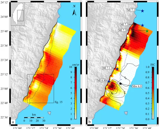
![Figure 6. (a) Secular motion of the Central Range (black arrows) and Coastal Range (green arrows) blocks relative to the Philippine Sea Plate, as defined by Philippine/ITRF [DeMets et al., 2011]](https://thumb-eu.123doks.com/thumbv2/123doknet/14772050.591745/12.918.290.839.135.498/figure-secular-central-coastal-relative-philippine-defined-philippine.webp)

Documents relatifs