HAL Id: hal-01162796
https://hal.inria.fr/hal-01162796
Submitted on 11 Jun 2015
HAL is a multi-disciplinary open access
archive for the deposit and dissemination of
sci-entific research documents, whether they are
pub-lished or not. The documents may come from
teaching and research institutions in France or
abroad, or from public or private research centers.
L’archive ouverte pluridisciplinaire HAL, est
destinée au dépôt et à la diffusion de documents
scientifiques de niveau recherche, publiés ou non,
émanant des établissements d’enseignement et de
recherche français ou étrangers, des laboratoires
publics ou privés.
Finding Paths in Grids with Forbidden Transitions
Mamadou Moustapha Kanté, Fatima Zahra Moataz, Benjamin Momège,
Nicolas Nisse
To cite this version:
Mamadou Moustapha Kanté, Fatima Zahra Moataz, Benjamin Momège, Nicolas Nisse. Finding Paths
in Grids with Forbidden Transitions. WG 2015, 41st International Workshop on Graph-Theoretic
Concepts in Computer Science, Jun 2015, Munich, Germany. �hal-01162796�
Finding Paths in Grids with Forbidden
Transitions
M. M. Kant´e1, F. Z. Moataz2,3?, B. Mom`ege2,3, and N. Nisse3,2
1
Univ. Blaise Pascal, LIMOS, CNRS, Clermont-Ferrand, France
2
Univ. Nice Sophia Antipolis, CNRS, I3S, UMR 7271, 06900 Sophia Antipolis, France
3
INRIA, France
Abstract. A transition in a graph is a pair of adjacent edges. Given a graph G = (V, E), a set of forbidden transitions F ⊆ E × E and two vertices s, t ∈ V , we study the problem of finding a path from s to t which uses none of the forbidden transitions of F . This means that it is forbidden for the path to consecutively use two edges forming a pair in F . The study of this problem is motivated by routing in road networks in which forbidden transitions are associated to prohibited turns as well as routing in optical networks with asymmetric nodes, which are nodes where a signal on an ingress port can only reach a subset of egress ports. If the path is not required to be elementary, the problem can be solved in polynomial time. On the other side, if the path has to be elementary, the problem is known to be NP-complete in general graphs [Szeider 2003]. In this paper, we study the problem of finding an elementary path avoiding forbidden transitions in planar graphs. We prove that the problem is NP-complete in planar graphs and particularly in grids. In addition, we show that the problem can be solved in polynomial time in graphs with bounded treewidth. More precisely, we show that there is an algorithm which solves the problem in time O((3∆(k + 1))2k+4n)) in n-node graphs
with treewidth at most k and maximum degree ∆.
1
Introduction
Driving in New-York is not easy. Not only because of the rush hours and the taxi drivers, but because of the no-left, no-right and no U-turn signs. Even in a “grid-like” city like New-York, prohibited turns might force a driver to cross several times the same intersection before eventually reaching their destination. In this paper, we give hints explaining why it is difficult to deal with forbidden-turn signs when driving in grid-like road networks.
Let G = (V, E) be a graph. A transition in G is a pair of two distinct edges incident to a same vertex. LetF ⊆ E × E be a set of forbidden transitions in G. We say that a not necessarily elementary path P = (v0, . . . , vq) is F-valid
if it contains none of the transitions of F, i.e., {{vi−1, vi}, {vi, vi+1}} /∈ F for
?
This author is supported by a grant from the ”Conseil r´egional Provence Alpes-Cˆote d’Azur”.
i ∈ {1, . . . , q − 1}. Given G, F and two vertices s and t, the Path Avoiding Forbidden Transitions (PAFT) problem consists in finding anF-valid s-t-path. The PAFT problem arises in many contexts. In optical networks for instance, nodes can be highly asymmetric with respect to their switching capabilities as pointed out in [2]. This means that an optical node might have some restrictions on its internal connectivity and that, consequently, signal on a certain ingress port can only reach a subset of the egress ports. As explained in [2, 4, 7], a node can be asymmetrically configured for many reasons such as the limitation on the number of physical ports of optical switch components and the low cost of asymmetric nodes compared to symmetric ones. The existence of asymmetric nodes adds some connectivity constraints in the network. This has motivated some studies to re-investigate, under the assumption of the existence of asym-metric nodes, some classical problems in optical network, such as routing [2, 4, 9] and protection with node-disjoint paths [7]. These studies do not highlight the computational complexity of the problems they consider. We point out here that the optical nodes configured asymmetrically can be modeled as vertices with forbidden transitions and the routing problem is an application of PAFT. The study of PAFT is also motivated by its relevance to vehicle routing. In road networks, it is possible that some roads are closed due to traffic jams, construc-tion, etc. It is also frequent to encounter no-left, no-right and no U-turn signs at intersections. These prohibited roads and turns can be modeled by forbidden transitions.
When the PAFT problem is studied, a distinction has to be made accord-ing to whether the path to find is elementary (cannot repeat vertices) or elementary. Indeed, PAFT can be solved in polynomial time [6] for the non-elementary case while finding an non-elementary path avoiding forbidden transitions has been proved NP-complete in [12]. In this paper, we study the elementary version of the PAFT problem in planar graphs and more particularly in grids. Our interest for planar graphs is motivated by the fact that they are closely re-lated to road networks. They are also an interesting special case to study while trying to capture the difficulty of the problem. Furthermore, to the best of our knowledge, this case has not been addressed before in the literature.
Related work PAFT is a special case of the problem of finding a path avoiding forbidden paths (PFP) introduced in [15]. Given a graph G, two vertices s and t, and a setS of forbidden paths, PFP aims at finding an s-t-path which contains no path of S as a subpath. When the forbidden paths are composed of exactly two edges, PFP is equivalent to PAFT. Many papers address the non-elementary version of PFP, proposing exact polynomial solutions [15, 8, 1]. The elementary counterpart has been recently studied in [10] where a mathematical formulation is given and two solution approaches are developed and tested. The computa-tional complexity of the elementary PFP can be deduced from the complexity of PAFT which has been established in [12]. Szeider proved in [12] that finding an elementary path avoiding forbidden transitions is NP-complete and gave a complexity classification of the problem according to the types of the forbidden transitions. The NP-completeness proof in [12] does not extend to planar graphs.
PAFT is also a generalization of the problem of finding a properly colored path in an edge-colored graph (PEC). Given an edge-colored graph Gc and
two vertices s and t, the PEC problem aims at finding an s-t-path such that any consecutive two edges have different colors. It is easy to see that PEC is equivalent to PAFT when the set of forbidden transitions consists of all pairs of adjacent edges that have the same color. The PEC problem is proved to be NP-complete in directed graphs [5] which directly implies that the PAFT problem is NP-complete in directed graphs4.
Contribution Our main contribution is the proof that the PAFT problem is NP-complete in grids. We also prove that the problem can be solved in time O((3∆(k + 1))2k+4n)) in n-node graphs with treewidth at most k and maximum
degree ∆. In other words, we prove that the PAFT problem is FPT in k + ∆. Our NP-completeness result strengthens the one of Szeider [12] established in 2003 and extends to the problem of PFP.
The paper is organized as follows. The problem of PAFT is formally stated in Section 2. In Section 3, the problem is proven NP-complete in grids. A polynomial time algorithm for graphs with bounded treewidth is presented in Section 4. Finally, some directions for future work are presented in Section 5
2
Problem statement
Let G = (V, E) be a graph. Given a subgraph H of G, a transition in H is a (not ordered) set of two distinct edges of H incident to a same vertex. Namely, {e, f} is a transition if e, f ∈ E(H), e 6= f and e ∩ f 6= ∅. Let T denote the set of all transitions in G. LetF ⊆ T be a set of forbidden transitions. A transition in A = T \ F is said allowed. A path is any sequence (v0, v1,· · · , vr) of vertices such
that vi 6= vj for any 0≤ i < j ≤ r and ei ={vi, vi+1} ∈ E for any 0 ≤ i < r.
Given two vertices s and t in G, a path P = (v0, v1,· · · , vr) is called an s-t-path if
v0= s and vr= t. Finally, a path P = (v0, v1,· · · , vr) isF-valid if any transition
in P is allowed, i.e.,{ei, ei+1} /∈ F for any 0 ≤ i < r.
Problem 1 (Problem of Finding a Path Avoiding Forbidden Transitions, PAFT). Given a graph G = (V, E), a set F of forbidden transitions and two vertices s, t∈ V . Is there an F-valid s-t-path in G?
3
NP-completeness in grids
We start by proving that the PAFT problem is NP-complete in grids. For this purpose, we first prove that it is NP-complete in planar graphs with maximum
4
Note that, in [5], the authors state that their result can be extended to planar graphs. However, there is a mistake in the proof of the corresponding Corollary 7: to make their graph planar, vertices are added when edges intersect. Unfortunately, this transformation does not preserve the fact that the path is elementary.
degree at most 8 by a reduction from 3-SAT. Then, we propose simple transfor-mations to reduce the degree of the vertices and prove that the PAFT problem is NP-complete in planar graphs with degree at most 4. Finally, we prove it is NP-complete in grids.
Lemma 1. The PAFT problem is NP-complete in planar graphs with maximum degree 8.
Proof. The problem is clearly in NP. We prove the hardness using a reduction from the 3-SAT problem. Let Φ be an instance of 3-SAT, i.e., Φ is a boolean for-mula with variables{v1,· · · , vn} and clauses {C1,· · · , Cm}. We build a grid-like
planar graph G where rows correspond to clauses and columns correspond to variables. In what follows, the colors are only used to make the presentation eas-ier. Moreover, we consider undirected graphs but, since the forbidden transitions can simulate orientations, the figures are depicted with directed arcs for ease of presentation. Please note also that we use a multigraph in the reduction for the sake of simplicity. This multigraph can easily be transformed into a simple graph without changing the maximum degree.
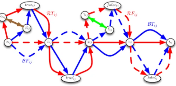
Gadget Gij. For any i≤ n and j ≤ m, we define the gadget Gij depicted in
Figure 1 and that consists of 4 edge-disjoint paths from sij to tij: two “blue”
pathsBTij andBFij, and two “red” pathsRTij andRFij defined as follows.
– RTij = (sij, αij, trueij, xij, true0ij, yij, zij, tij);
– BTij= (sij, βij, trueij, xij, true0ij, yij, zij, tij);
– RFij = (sij, xij, yij, γij, f alseij, zij, f alse0ij, tij);
– BFij = (sij, xij, yij, δij, f alseij, zij, f alse0ij, tij).
The forbidden transitions Fij of the gadget Gij are defined in such a way
that the only way to go from sij to tij is by following one of the paths in
{BTij,BFij,RTij,RFij}. It is forbidden to use any transition consisting of two
edges from two different paths of the set{BTij,BFij,RTij,RFij}.
Intuitively, assigning the variable vi to T rue will be equivalent to choosing
one of the pathsBTij orRTij (called positive paths) depicted with full lines in
Fig. 1. Respectively, assigning vi to F alse will correspond to choosing one of the
pathsBFij orRFij(called negative paths) and depicted by dotted line in Fig. 1.
So far, it is a priori not possible to start from sij by one path and arrive
in tij by another path. In particular, the color by which sij is left must be
the same by which tij is reached. If Variable vi appears in Clause Cj, we add
one edge to Gij as follows. If vi appears positively in Cj, we add the brown
edge {αij, βij} that creates a “bridge” between BTij and RTij. Similarly, if vi
appears negatively in Cj, we add the green edge{γij, δij} that creates a “bridge”
between BFij and RFij. When the gadget Gij contains a brown (resp. green)
edge, all the transitions containing the brown (resp. green) edge are allowed; this makes it possible to switch between the positive (resp. negative) pathsBTij
andRTij (resp.BFij andRFij) when going from sij to tij. Hence, if vi appears
sij xij yij zij tij f alseij trueij true� ij f alse�ij αij βij γij δij BTij RTij BFij RFij
Fig. 1: Example of the Gadget-graph Gij for Variable vi, and j ≤ m. Brown
(resp. green) edge is added if vi appears positively (resp., negatively) in Cj. If
vi ∈ C/ j, none of the green nor brown edge appear.
a different one. Note that, the type of path (positive or negative) cannot be modified between sij and tij.
We characterize theFij-valid sij-tij-paths in Gij with the following
straight-forward claims.
Claim 1 TheFij-valid sij-tij-paths in Gij are RTij,BTij,RFij,BFij and
– if variable vi appears positively in ClauseCj:
• the path RBTij that starts with the first edge {sij, αij} of RTij, then
uses brown edge {αij, βij} and ends with all edges of BTij but the first
one;
• the path BRTij that starts with the first edge{sij, βij} of BTij, then uses
brown edge {αij, βij} and ends with all edges of RTij but the first one;
– if variable vi appears negatively in ClauseCj:
• the path RBFij that starts with the subpath (sij, xij, yij, γij) of RFij,
then uses green edge {γij, δij} and ends with the subpath of BFij that
starts atδij and ends attij;
• the path BRFij that starts with the subpath (sij, xij, yij, δij) of BFij,
then uses green edge {δij, γij} and ends with the subpath of RFij that
starts atγij and ends attij;
Claim 2 LetP be a Fij-validsijtij-paths inGij. Then, either
– P passes through trueij and true0ij and does not pass through f alseij nor
f alse0 ij, or
– P passes through f alseij andf alse0ij and does not pass through trueij nor
true0 ij.
Claim 3 Let P be aFij-validsijtij-paths inGij. Then the first and last edges
of P have different colors if and only if P uses a green or a brown edge, i.e., if P ∈ {RBTij,BRTij,RBFij,BRFij}.
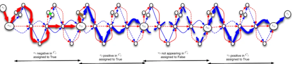
Clause-graphGj. For any j≤ m, the Clause-gadget Gj is built by combining
the graphs Gij, i≤ n, in a “line” (see Fig. 2). The subgraphs Gij are combined
from “left to right” (for i = 1 to n) if j is odd and from “right to left” (for i = n to 1) otherwise. In more details, for any j ≤ m, Gj is obtained from a copy of
each gadget Gij, 1≤ i ≤ n, and two additional vertices sj and tj as follows:
– If j is odd, the subgraph Gj starts with a red edge {sj, s1j} and then, for
1 < i≤ n, the vertices sij and ti−1,j are identified. Finally, there is a blue
edge from tnj to vertex tj.
– If j is even, the subgraph Gj starts with a blue edge{sj, snj} and then, for
1 < i≤ n, the vertices tij and si−1,j are identified. Finally, there is a red
edge from t1j to vertex tj.
The forbidden transitions Fj include, besides all transitions in Fij, i =
1, . . . , n , new transitions which are defined such that, when passing from a gadget Gij to the next one, the same color must be used. This means that if we
enter a vertex tij = si,j+1 by an edge with a given color, the same color must
be used to leave this vertex. However, in such vertices, we can change the type (positive or negative) of path.
Note that if we enter a Clause-graph with a red (resp. blue) edge, we can only leave it with a blue (resp. red) edge. This means that a path must change its color inside the Clause-graph, and must hence use a brown or green edge in some gadget-graph. The use of a brown (resp. green) forces a variable that appears positively (resp. negatively) in the clause to be set to true (resp. false) and validates the Clause.
The key property of Gj relates to the structure ofFj-valid paths from sj to
tj, which we summarize in Claims 4 and 5.
Claim 4 AnyFj-valid pathP from sj totj inGj consists of the concatenation
of:
Case j odd. the red edge {sj, s1j}, then the concatenation of Fij-valid paths
from sij to tij in Gij, for 1 ≤ i ≤ n in this order (from i = 1 to n), and
finally the blue edge{tnj, tj};
Case j even. the blue edge{sj, snj}, then the concatenation of Fij-valid paths
fromsij totij inGij, for 1≤ i ≤ n in the reverse order (from i = n to 1),
and finally the red edge{t1j, tj}.
By the previous claim, for anyFj-valid path P from sj to tj, the colors of the
first and last edges differ. Hence, by Claim 3 and the definition of the allowed transitions between two gadgets:
Claim 5 Any Fj-valid pathP from sj totj must use a green or a brown edge
t3j
t2j
v1 negative in Cj
assigned to True v2 positive in Cj
assigned to True
v3 not appearing in Cj
assigned to False v4 positive in Cj
assigned to True
s1j t1j t4j
sj
tj
Fig. 2: Case j odd. Clause-graph Gj for a Clause Cj= ¯v1∨ v2∨ v4in a formula
with 4 Variables. The bold path corresponds to an assignment of v1, v2 and v4
to T rue, and of v3 to F alse.
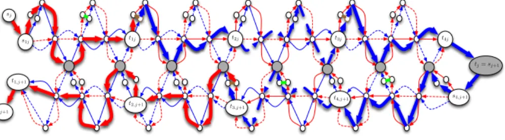
Main graph. To conclude, we have to be sure that the assignment of the variables is coherent between the clauses. For this purpose, let us combine the subgraphs Gj, j ≤ m, as follows (see Fig 3). First, for any 1 ≤ j < m, let
us identify tj and sj+1. Then, some vertices (depicted in grey in Fig 3) of Gij
are identified with vertices of Gi,j+1 in such a way that using a positive (resp.,
negative) path in Gij forces the use of the same type of path in Gi,j+1. That
is, the choice of the path used in Gij is transferred to Gi,j+1 and therefore it
corresponds to a truth assignment for Variable vi.
Namely, for each 1≤ j < m and for each 1 ≤ i ≤ n, we identify the vertices truei,j+1 and f alse0ij on the one hand, and the vertices true0ij and f alsei,j+1 on
the other hand to obtain the ”grey” vertices. Finally, forbidden transitionsF of G, include, besides all transitions inFj for j = 1, . . . , m, new transitions which
are defined in order to forbid “crossing” a grey vertex, i.e., it is not possible to go from Gi,j to Gi,j+1 via a grey vertex. The following claims present the key
properties of anF-valid path in G.
Claim 6 AnyF-valid path P from s1 totm inG consists of the concatenation
of Fj-valid paths fromsj totj inGj from j = 1 to m.
Claim 7 LetP be an F-valid s1tm-path inG. Then, for any 1≤ i ≤ n, either
– for any 1 ≤ j ≤ m, the subpath of P between sij and tij passes through
trueij and true0ij and does not pass throughf alseij nor f alse0ij, or
– for any 1 ≤ j ≤ m, the subpath of P between sij and tij passes through
f alseij andf alse0ij and does not pass throughtrueij nor true0ij.
Proof. By Claims 4 and 6, for any 1≤ i ≤ n and any 1 ≤ j ≤ m, there is a subpath Pij of P that goes from sij to tij. Moreover, the paths Pij are pairwise
vertex-disjoint.
For 1≤ i ≤ n, by Claim 2, Pi1 either passes through truei1 and true0i1, or
through f alsei1 and f alse0i1. Let us assume that we are in the first case (the
second case can be handled symmetrically). We prove by induction on j ≤ m that Pijpasses through trueij and true0ij and does not pass through f alseij nor
f alse0 ij.
Indeed, if P passes through trueij = f alse0i,j+1 and true0ij = f alsei,j+1,
then Pi,j+1 cannot use f alsei,j+1 nor f alse0i,j+1 since Pij and Pi,j+1 are
vertex-disjoint. By Claim 2, Pi,j+1 passes through truei,j+1 and true0i,j+1.
u t sj s1j t1j t2j t3j t4j tj= sj+1 s4,j+1 t4,j+1 t3,j+1 t2,j+1 t1,j+1 tj+1
Fig. 3: Combining Cj = ¯v1∨ v2∨ v4 and Cj+1= v2∨ ¯v3∨ ¯v4 (Case j odd).
Note that (G,F) can be constructed in polynomial-time. Moreover, G is clearly planar with maximum degree 8. Hence, the next claim allows to prove Lemma 1.
Claim 8 Φ is satisfiable if and only if there is anF-valid s1-tm-path inG.
Proof. Let ϕ be a truth assignment which satisfies Φ. We can build an F-valid s1-tm-path in G as follows. For each row 1≤ j ≤ m, we build a path Pj from
si to tj by concatenating the paths Pij, 1≤ j ≤ m, which are built as follows.
Among the variables that appear in Cj, let vk be the variable with the smallest
index, which satisfies the clause.
– For 1≤ i < k, if ϕ(vi) = true, then Pij =RTij if j is odd and Pij =BTij
if j is even, respectively. If ϕ(vi) = f alse, then Pij =RFij if j is odd, and
Pij =BFij if j is even.
– If ϕ(vk) = true, then Pij =RBTij if j is odd, and Pij=BRTij if j is even.
If ϕ(vk) = f alse, then Pij =RBFij if j is odd, and Pij =BRFij if j is even.
– For k < i≤ n, if ϕ(vi) = true, then Pij =BTij if j is odd, and Pij =RTij
if j is even. If ϕ(vi) = f alse, then Pij =BFij if j is odd, and Pij =RFij
otherwise.
The path P obtained from the concatenation of paths Pj for 1≤ j ≤ m is an
F-valid path from s1to tm.
Now let us suppose that there is anF-valid path P from s1to tm. According
to Claim 7, for any 1≤ i ≤ n, for any 1 ≤ j ≤ m, P passes through trueij and
true0ij or for any 1≤ j ≤ m, P passes through falseij and f alse0ij. Let us then
consider the truth assignment ϕ of Φ such that for each 1≤ i ≤ n: – If P uses trueij and true0ij in all rows 1≤ j ≤ m, then ϕ(vi) = true.
– If P uses f alseij and f alse0ij in all rows 1≤ j ≤ m, then ϕ(vi) = f alse.
Thanks to Claim 7, ϕ is a valid truth assignment. We need to prove that ϕ satisfies Φ. According to Claim 6, for each row 1≤ j ≤ m, P contains an Fj
-valid path Pj from sj to tj. Each path Pjuses a green or a brown edge as stated
by Claim 3. With respect to the possible ways to use a green or a brown edge which are stated in Claim 2, the use of a brown edge in Pj forces Pj (and hence
P ) to use, for a variable vithat appears positively in Cj, the vertices trueij and
true0
ij. Similarly, the use of a green edge in Pjforces Pj (and hence P ) to use, for
a variable vithat appears negatively in Cj, the vertices f alseijand f alce0ij. This
means that for each clause Cj, for one of the variables that appear in Cj which
we denote vi, ϕ(vi) = true (ϕ(vi) = f alse) if vi appears positively (negatively)
in Cj, respectively. Thus, the truth assignment ϕ satisfies Φ. ut
Due to lack of space, we only give a sketch of the proof of the next lemma. The full proof can be found in the Appendix.
Lemma 2. The PAFT problem is NP-complete in planar graphs with maximum degree 4.
Proof (sketch). The graph G used in the reduction of the proof of Lemma 1 is planar and each vertex of G has either degree 8, degree 5 or degree at most 4. We transform G into a planar graph G0 with maximum degree 4 and an
associated set of forbidden transitions F0 such that finding anF-valid path in
G is equivalent to finding anF0-valid path in G0:
– We transform vertices of degree 5 to vertices of degree 3 as follows. For vertices s1j (resp. t1j) where j is odd we delete the 2 blue edges incident to
s1j (resp. t1j). For vertices snj (resp. t1j) where j is even, we delete the 2
red edges incident to snj (resp. t1j).
– We replace each vertex v of degree 8 by a gadget gv of maximum degree 4.
Gadget gv is designed such that it can be crossed at most once by a path of
G0 and only if the edges used to enter and leave g
vcorrespond to an allowed
transition around v. Figure 5 gives an example of a vertex v in G and the corresponding gadget gv in G0. ut
Theorem 1. The problem of finding a path avoiding forbidden transitions is NP-complete in grids.
Proof. To prove the theorem we use the notion of planar grid embedding [13]. A planar grid embedding of a graph G is a mapping Q of G into a grid such that Q maps each vertex of G into a distinct vertex of the grid and each edge e of G into a path of the grid Q(e) whose endpoints are mappings of vertices linked by e. For every pair {e, e0} of edges of G, the corresponding paths Q(e) and Q(e0)
have no points in common, except, possibly, the endpoints. It has been proved in [14], that if G = (V, E) is a planar graph such that |V | = n and ∆ ≤ 4, then a planar grid embedding of G in a grid of size at most 9n2 can be found in
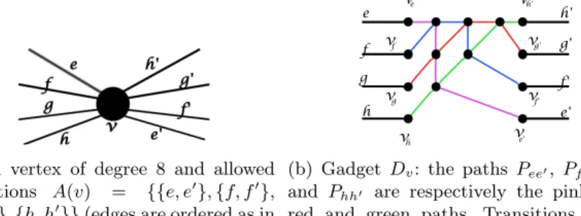
e f g h e' f' g' h' v
(a) A vertex of degree 8 and allowed transtions A(v) = {{e, e0}, {f, f0},
{g, g0}, {h, h0}} e f g h e' f' g' h' v v v v v v v ve f g h h' g' f' e'
(b) Gadget gv: the paths Pee0, Pf f0,Pgg0,
and Phh0 are respectively the pink,
yel-low, black and green paths. Only transitions around vertices vi and transitions of paths
Pee0, Pf f0,Pgg0, and Phh0 are allowed
Fig. 4: Example of a vertex v and the corresponding gadget gv
polynomial-time. Let us consider an instance of the problem of finding a path avoiding forbidden transitions in a planar graph G = (V, E) of maximum degree at most 4 with a set of allowed transitionsA (A = E × E \ F). Let Q be a grid planar embedding of G into a grid K of size at most O(|V |2). Finding a PAFT
between two nodes s and t in G with the setA is equivalent to finding a PAFT between the nodes Q(s) and Q(t) in K with the set of allowed transitions A0
defined such that:
– For each e∈ E, all the transitions in the path Q(e) are allowed.
– For each {e, e0} ∈ A, the pair of edges of Q(e) and Q(e0), which share a vertex, is an allowed transition.
u t
4
Parameterized complexity
On the positive side, by using dynamic programming on a tree-decomposition of the input graph, we prove that the problem is FPT when the parameter is the sum of the treewidth and the maximum degree.
A tree-decomposition of a graph [11] is a way to represent G by a family of subsets of its vertex-set organized in a tree-like manner and satisfying some connectivity property. The treewidth of G measures the proximity of G to a tree. More formally, a tree decomposition of G = (V, E) is a pair (T,X ) where X = {Xt|t ∈ V (T )} is a family of subsets, called bags, of V , and T is a tree,
such that: S
t∈V (T )Xt = V , for any edge uv ∈ E, there is a bag Xt (for some
node t ∈ V (T )) containing both u and v, and for any vertex v ∈ V , the set {t ∈ V (T )|v ∈ Xt} induces a subtree of T . The width of a tree-decomposition
(T,X ) is maxt∈V (T )|Xt|−1 and its size is order |V (T )| of T . The treewidth of G,
denoted by tw(G), is the minimum width over all possible tree-decompositions of G.
Theorem 2 proves that when the treewidth of the graph is bounded, the PAFT can be solved in polynomial time. Complete proof of the theorem can be found in the Appendix.
Theorem 2. The problem of finding a path avoiding forbidden transitions is FPT when parameterized by k + ∆ where k is the treewidth and ∆ is the maxi-mum degree. In particular, there exists an algorithm that finds the shortest path avoiding forbidden transitions between two vertices in timeO((3∆(k+1))2k+4n))
The Algorithm uses dynamic programming techniques and its key idea is similar to the one used to find a Hamiltonian cycle in graphs with bounded treewidth [3].
In more details, let G = (V, E) be a graph with bounded treewidth k, F a set of forbidden transitions , and s and t two vertices of V . Let (T,X ) be a tree-decomposition of width k of G rooted in an arbitrary node. Let G[A] be the subgraph of G induced by the set of vertices A. For each u∈ V (T ), we denote by Xu,Tu and Vu the set of vertices of the bag corresponding to u, the subtree
of T rooted at u, and the set of vertices of the bags corresponding to the nodes of Tu , respectively.
If there exists an F-valid path P from s to t, then the intersection of this path with G[Vu] for a node u∈ T consists of a set of paths avoiding forbidden
transitions each having both endpoints in Xu. If t∈ Vu, then one of the paths
has only one endpoint in Xu. With respect to the parts of path P that are in
G[Vu], vertices in Xucan be partitioned into three subsets Xu0, Xu1, and Xu2which
are the vertices of degree 0, 1 and 2 in P ∩ G[Vu], respectively. Furthermore, a
matching M of X1
udecides which vertices are endpoints of the same subpath and
a set of edges S defines which edges incident to X1
uare in P . For each node u∈ T
and each subproblem (X0
u, Xu1, Xu2, M, S) where (Xu0, Xu1, Xu2) is a partition of
Xu, M is a matching of Xu1 and S is a set of edges incident to the vertices of
X1
u, we need to check if there exists a set of paths avoiding forbidden transitions
in Vu such that their endpoints are exactly Xu1 according to the matching M ,
they contain the edges of S and the vertices of X2
u and they do not contain any
vertex of X0
u. For each node, we will need to solve at most 3k+1(k + 1)k+1∆k+1
subproblems; there are at most 3k+1 possible partitions of the vertices of X u
into the 3 different sets, (k + 1)k+1possible matchings for a set of k + 1 elements
and ∆ possible edges for each element of X1 u.
5
Conclusion
We have proven that the problem of finding a path avoiding forbidden transi-tions is NP-complete even in well-structured graphs as grids. We have also proved that PAFT can be solved in polynomial time when the treewidth is bounded. We believe that the PAFT is actually W [1]-hard when parameterized by the treewidth. Future work might focus on proving this conjecture and also on us-ing structural properties of planar graphs to improve the runnus-ing time of the algorithm for solving PAFT in planar graphs with bounded treewidth. Another
interesting direction in the study of PAFT could be to consider the optimization problem where the objective is to find a path with minimum number of forbidden transitions and to investigate possible approximation solutions.
References
1. Ahmed, M., and Lubiw, A. Shortest paths avoiding forbidden subpaths. Networks 61, 4 (2013), 322–334.
2. Bernstein, G., Lee, Y., Gavler, A., and Martensson, J. Modeling WDM wavelength switching systems for use in GMPLS and automated path computation. Optical Communications and Networking, IEEE 1, 1 (June 2009), 187–195. 3. Bodlaender, H. Dynamic programming on graphs with bounded treewidth. In
Automata, Languages and Programming, vol. 317 of Lecture Notes in Computer Science. Springer Berlin Heidelberg, 1988, pp. 105–118.
4. Chen, Y., Hua, N., Wan, X., Zhang, H., and Zheng, X. Dynamic lightpath provisioning in optical wdm mesh networks with asymmetric nodes. Photonic Network Com. 25, 3 (2013), 166–177.
5. Gourv`es, L., Lyra, A., Martinhon, C. A., and Monnot, J. Complexity of trails, paths and circuits in arc-colored digraphs. Discrete Applied Mathematics 161, 6 (2013), 819 – 828.
6. Guti´errez, E., and Medaglia, A. L. Labeling algorithm for the shortest path problem with turn prohibitions with application to large-scale road networks. An-nals of Operations Research 157, 1 (2008), 169–182.
7. Hashiguchi, T., Tajima, K., Takita, Y., and Naito, T. Node-disjoint paths search in wdm networks with asymmetric nodes. In Optical Network Design and Modeling (ONDM), 2011 15th International Conference on (Feb 2011), pp. 1–6. 8. Hsu, C.-C., Chen, D.-R., and Ding, H.-Y. An efficient algorithm for the shortest
path problem with forbidden paths. In Algorithms and Architectures for Parallel Processing, A. Hua and S.-L. Chang, Eds., vol. 5574 of Lecture Notes in Computer Science. Springer Berlin Heidelberg, 2009, pp. 638–650.
9. Jaumard, B., and Kien, D. Optimizing roadm configuration in wdm networks. In Telecommunications Network Strategy and Planning Symposium (Networks), 2014 16th International (Sept 2014), pp. 1–7.
10. Pugliese, L. D. P., and Guerriero, F. Shortest path problem with forbidden paths: The elementary version. European Journal of Operational Research 227, 2 (2013), 254 – 267.
11. Robertson, N., and Seymour, P. D. Graph minors. II. algorithmic aspects of tree-width. J. Algorithms 7, 3 (1986), 309–322.
12. Szeider, S. Finding paths in graphs avoiding forbidden transitions. Discrete Applied Mathematics 126, 2 - 3 (2003), 261 – 273.
13. Tamassia, R. On embedding a graph in the grid with the minimum number of bends. SIAM J. Comput. 16, 3 (June 1987), 421–444.
14. Valiant, L. G. Universality considerations in VLSI circuits. IEEE Transactions on Computers 30, 2 (1981), 135–140.
15. Villeneuve, D., and Desaulniers, G. The shortest path problem with forbidden paths. European Journal of Operational Research 165, 1 (2005), 97 – 107.
Appendix
We provide in this appendix the proofs of Lemma 2 and Theorem 2.
A Proof of Lemma 2
Let G be the graph obtained from the reduction in the proof of lemma 1 and letE be the planar embedding of G that is obtained by embedding the smaller gadgets as in Figures 1,2,3. the graph G has the following properties:
– G is planar.
– Each vertex of G has either degree 8 or degree≤ 4. In fact, there are also vertices of degree 5 which we transform to vertices of degree 3 as follows. For vertices s1j (resp. t1j) where j is odd we delete the 2 blue edges incident
to s1j (resp. t1j). For vertices snj (resp. t1j) where j is even, we delete the
2 red edges incident to snj (resp. t1j). This transformation does not affect
the reduction or the proof.
– According to its forbidden transitions and to its disposition in the planar embeddingE, a vertex v of G of degree 8 has one of three following types: Type 1: The edges incident to v are ω(v) ={e, e0, f, f0, g, g0, h, h0} and the
allowed transitions around v are A(v) ={{e, e0}, {f, f0}, {g, g0}, {h, h0}}.
The edges of v in the planar embeddingE. (v is a vertex of type xij, yij
or zij in the graph G)
Type 2: The edges incident to v are ω(v) ={e, e0, f, f0, g, g0, h, h0} and the
allowed transitions around v are A(v) ={{e, e0}, {f, f0}, {g, g0}, {h, h0}}.
The edges of v in the planar embeddingE. (v is a vertex of type trueij,
true0
ij, f alseij, or f alse0ij in the graph G)
Type 3: The edges incident to v are ω(v) ={e, e0, f, f0, g, g0, h, h0} and the
allowed transitions around v are A(v) ={{e, e0}, {e, f0}, {f, f0}, {f, e0},
{g, g0}, {g, h0}, {h, h0}, {h, g0}}. The edges of v in the planar embedding
E are as depicted in Figure7a. (v is a vertex of type sij in the graph G)
To prove the lemma, we are going to replace each vertex v of degree 8 in G with a gadget Dv. After replacing all vertices of degree 8, we will obtain a graph
G0 of maximum degree 4 and a new set of forbidden transitions F0 such that
finding an F−valid path from s to t in G is equivalent to finding an F0-valid
path from s to t in G0. Let v be a vertex of degree 8 of G. D
v is constructed
according to the type of v as follows:
Type 1 In this case, Dv is constructed as follows. For each i∈ ω(v), a vertex vi
is created. For each{i, j} ∈ A(v), vertices vi and vj are linked with a path
Pij of length four . The four paths Pij are pairwise intersecting in distinct
vertices as illustrated in Figure 5b. The allowed transitions in Dv are the
transitions of the paths Pij. Now to replace v with Dv in G, we do the
following: each edge i∈ ω(v) of G is linked to vertex vi of Dv. The gadget
Dvis planar, and edges i∈ ω(v) are connected to it in the same ”order” they
Note the gadget Dv cannot be crossed twice with the same path, otherwise
the path is not simple. Moreover, Dv can be crossed if and only if the edges
used to enter and leave form an allowed transition around v.
(a) A vertex of degree 8 and allowed transtions A(v) = {{e, e0}, {f, f0}, {g, g0}, {h, h0}} (edges are ordered as in
the planar embedding E of G)
e f g h e' f' g' h' v v v v v v v ve f g h h' g' f' e'
(b) Gadget Dv: the paths Pee0, Pf f0,Pgg0,
and Phh0 are respectively the pink, blue,
red and green paths. Transitions around vertices vi and transitions of paths Pee0,
Pf f0,Pgg0, and Phh0 are allowed
Fig. 5: Type 1
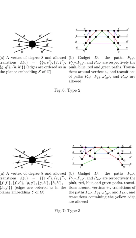
Type 2 In this case, Dv is constructed as follows. For each i∈ ω(v), a vertex vi
is created. For each{i, j} ∈ A(v), vertices vi and vj are linked with a path
Pij of length 7 . Each two of the four paths Pij intersect in two different
vertices as illustrated in Figure 6b. The allowed transitions in Dv are the
transitions of the paths Pij. Now to replace v with Dv in G, we do the
following: each edge i∈ ω(v) of G is linked to vertex vi of Dv. The gadget
Dv is planar, and edges i ∈ ω(v) are connected to it in the same ”order”
they were connected to v in the planar embeddingE of G as illustrated in Figure 6. Note that the gadget Dv cannot be crossed twice with the same
path, otherwise the path is not simple. Moreover, Dv can be crossed if and
only if the edges used to enter and leave form an allowed transition around v.
Type 3 In this case, Dv is constructed as follows. For each{i, i0} ∈ A(v) ,
ver-tices viand vj are linked with a path Pij of length 7. Each two of the paths
Pij intersect twice in distinct vertices as illustrated in Figure 7b.
Further-more, we add two edges linking the paths Pee0 and Pf f0, and Pgg0 and Phh0,
respectively. Now to replace v with Dv in G, we do the following: each edge
i ∈ ω(v) of G is linked to vertex vi of Dv. The gadget Dv is planar, and
edges i∈ ω(v) are connected to it in the same ”order” they were connected to v in the planar embeddingE of G as illustrated in Figure 7. Note that the gadget Dv cannot be crossed twice with the same path, otherwise the path
is not simple. Moreover, Dv can be crossed if and only if the edges used to
enter and leave form an allowed transition around v.
The graph G0 is the one obtained from G after replacing vertices of degree
(a) A vertex of degree 8 and allowed transtions A(v) = {{e, e0}, {f, f0}, {g, g0}, {h, h0}} (edges are ordered as in
the planar embedding E of G)
e f g h e' f' g' h' ve vf vg vh vh' vg' vf' ve'
(b) Gadget Dv: the paths Pee0,
Pf f0,Pgg0, and Phh0are respectively the
pink, blue, red and green paths. Transi-tions around vertices viand transitions
of paths Pee0, Pf f0,Pgg0, and Phh0 are
allowed Fig. 6: Type 2
(a) A vertex of degree 8 and allowed transtions A(v) = {{e, e0}, {e, f0},
{f, f0}, {f, e0}, {g, g0}, {g, h0}, {h, h0}, {h, g0}} (edges are ordered as in the
planar embedding E of G) e f g h e' f' g' h' ve vf vg vh vh' vg' vf' ve'
(b) Gadget Dv: the paths Pee0,
Pf f0,Pgg0, and Phh0are respectively the
pink, red, blue and green paths. transi-tions around vertices vi, transitions of
the paths Pee0, Pf f0,Pgg0, and Phh0, and
transitions containing the yellow edge are allowed
of the transitions of the set F and the forbidden transitions of the gadgets Dv
as described above. The maximum degree of G0 is 4 and G0 is planar.
Let us now suppose that there is an F-valid path P from s to t in G. Let P0 be the s-t-path of G0 constructed as follows: P0 uses all edges used by P .
Furthermore, if P uses a degree 8 vertex of type 1 or 2 with a transition{e, e0}
then P0 uses e, subpath P
ee0, and e0. If P uses a degree 8 vertex of type 3 with
transition{e, e0} (or {e, f0}), then P0 uses e, e0 and the subpath P
ee0 (e,f0, and
the subpath Pef0 which is the concatenation of a subpath of path Pee0, a yellow
edge and a subpath of path Pee0), respectively. The path P0 isF0-valid.
Now, let us suppose that there is anF0-valid path P0 from s to t in G0. If P0 only uses edges from G, then it can be considered as anF-valid path from s to t in G. If P0 uses an edge that is not in G, then P0crosses one of the gadgets Dv.
As we have specified above, the gadgets Dvcan only be crossed in specified ways
that ensure that the edges used to enter and leave the gadget form an allowed transition. We can then remove the edges of P0that do not belong to G to obtain anF-valid path P in G. For any v of degree 8, the path P does not pass twice through v since gadget Dv in G0 cannot be crossed twice by the same path.
B Proof of Theorem 2
To prove theorem 2, we first introduce the following definition and lemma. Definition 1. A rooted tree decomposition ((T,X ), r) of G is nice if for every nodeu∈ V (T ):
– u has no children and|Xu| = 1 (u is called a leaf node), or
– u has one child v with Xu ⊂ Xv and |Xu| = |Xv| − 1 (u is called a forget
node),or
– u has one child v with Xv⊂ Xuand|Xu| = |Xv|+1 (u is called an introduce
node), or
– u has two children v and w with Xu= Xv = Xw (u is called a join node.).
Lemma 3. When given a tree decomposition of width w of G, in polynomial time we can construct a nice tree decomposition (T,X ) of G of width k, with |V (T )| ∈ O(kn), where n = |V (G)|.
We use the notion of nice tree decomposition and adapt the dynamic pro-gramming algorithm for finding a Hamiltonian cycle in a graph to prove Theo-rem 2.
Let G = (V, E) be a graph with bounded treewidth k, F ⊆ E × E a set of forbidden transitions (andA ⊆ E ×E the set of allowed transitions), and s and t two vertices of V . We would like to find the shortest path P from s to t avoiding the forbidden transitionsF.
Let Ge,f such that e and f are edges incident to s and t, respectively, be the
graph obtained from G, by deleting all edges incident to s and t except for e and f . Finding the shortest path avoiding forbidden transitionsF from s to t in G is equivalent to finding the shortest path among all shortest paths avoiding
forbidden transitions F from s to t in Ge,f, for each possible pair e, f . In the
following we will present how to solve the CFT problem in Ge,f. To obtain the
solution in G, we will need to repeat the algorithm at most ∆2times.
Let (T,X ) be a nice tree-decomposition of width k of Ge,f. We assume that
s appears in one introduce bag and t in two bags, a leaf and its introduce parent. We root T at the node containing s. Let G[A] be the subgraph of Ge,f induced
by the set of vertices A. . For each u∈ V (T ) we denote by Xu,Tu and Vu the
vertices of the bag corresponding to u, the subtree of T rooted at u, and the vertices of the bags corresponding to the nodes of Tu , respectively.
If there exists anF-valid path P from s to t, then the intersection of this path with G[Vu] for a node u ∈ T is a set of paths (avoiding forbidden transitions)
each having both endpoints in Xu. If t∈ Vu, then one of the paths has only one
endpoint in Xu.
With respect to the parts of path P that are in G[Vu], vertices in Xu can
be partitioned into three subsets: X0
u, Xu1, and Xu2 which are the vertices of
degree 0, 1 and 2 in P∩ G[Vu], respectively. Furthermore, a matching M of Xu1
decides which vertices are endpoints of the same subpath and a set of edges S defines which edges incident to X1
u are in P . For each node u ∈ T and each
subproblem (X0
u, Xu1, Xu2, M, S) where (Xu0, Xu1, Xu2) is a partition of Xu, M is a
matching of X1
u and S is a set of edges incident to the vertices of Xu1, we need
to see if there exists a set of paths avoiding forbidden transitions in Vu such
that their endpoints are exactly X1
u according to the matching M , they contain
the edges of S and the vertices of X2
u and they do not contain any vertex of
X0
u. For the case where t∈ Vu, we will need to check the possible matchings of
each subset of X1
uof size|Xu1| − 1. For each node, we will need to solve at most
3k+1(k + 1)k+1∆k+1subproblems; there are at most 3k+1possible partitions of
the vertices of Xu into the 3 different sets, (k + 1)k+1 possible matchings for a
set of k + 1 elements and ∆ possible edges for each element of X1 u.
Let us see how to solve a problem (X0
u, Xu1, Xu2, M, S) at a node u supposing
that all the problems at its descendants have been solved:
– If u is a leaf, then Xu = {a}. The only problem that has a solution is
(X0
u={a}, Xu1=∅, Xu2=∅, M = ∅, S = ∅).
– If u is a forget node, let v be the child of u. We have Xu= Xv\ a. We can
distinguish two cases:
• If a 6= t, then the problem (X0
u, Xu1, Xu2, M, S) has a solution if and
only if one of the problems (X0
u∪ {a}, Xu1, Xu2, M, S) and (Xu0, Xu1, Xu2∪
{a}, M, S) at node v has a solution. • If a = t, then the problem (X0
u, Xu1, Xu2, M, S) has a solution if and only
if the problem (X0
u, Xu1∪ {a}, Xu2, M, S) at v has a solution.
– If u is an introduce node, let v be the child of u. We have Xu= Xv∪ a (all
neighbors of a in Vu are in Xu). Note that a6= t since t appears in a forget
node and its introduce parent. In this case we proceed as follows. • If a ∈ X0
u, then solving (Xu0, Xu1, Xu2, M, S) at u is equivalent to solving
(X0
• if a ∈ X1
u, let ab be the edge incident to a in S. Since all neighbors of a
in Vu are in Xu, then b∈ Xu∩ Xv. Let us consider the following cases:
∗ If b = t, then the only problem that has a solution at u is (Xu\
{a, t}, {a, t}, ∅, {(a, t)}, {(a, t)}). To solve it, we need to check at v the solution of the problem (Xu\ {a}, ∅, ∅, ∅, ∅).
∗ If b ∈ X1
u (b6= t), (the problem has a solution only if (a, b) ∈ M and
the edge incident to b in S is ab) then check at v the solution of the problem (Xu0∪ {b}, Xu1\ {a, b}, Xu2, M0, S0) where M0 = M \ (a, b)
and S0 = S\ ab.
∗ If b ∈ X2
u (b 6= t), then check at v the solution of the problem
(X0
u, Xu1\ {a} ∪ {b}, Xu2\ {b}, M0, S0) where M0= M\ (a, h) ∪ (b, h)
and S0 contains the set S minus the edge ab plus an edge incident to
b that forms an allowed transition with edge ba (there are at most ∆ such problems).
• If a ∈ X2
u, then for every two neighbors b and c of a in Xu such that
(ba, ac) is an allowed transition do the following. ∗ If b ∈ X1
u and c ∈ Xu1, then check the solution at v of the problem
(X0
u∪ {b, c}, Xu1\ {b, c}, Xu2\ {a}, M0, S0) where M0= M\ (b, c) and
remove ab and bc from S to obtain S0. ∗ If b ∈ X2
u and c ∈ Xu2, then check the solution at v of the problem
(X0
u, Xu1∪{b, c}, Xu2\{a, b, c}, M0, S0) where M0= M∪{bh, ch0}\hh0
(bc should not be in the matching) and to obtain S0, add to S two edges incident to b and c and forming allowed transitions with ab and ac, respectively (there are k+1
2 possible choices for hh0 and ∆ 2
possible choices for the two edges to add to S). ∗ If b ∈ X1
u and c ∈ Xu2, then check the solution at v of the problem
(X0
u∪ {b}, Xu1\ {b} ∪ {c}, Xu2\ {a, c}, M0, S0) where M0 = M\ bh ∪ ch
and to obtain S0 remove ab from S and add an edge incident to c
that forms an allowed transition with ca. (There are ∆ possibilities). Note that the number of pairs of neighbors of a to consider are of order of k2.
– If u is a join node, let v and w be its children. For any two subproblems at v and w we check if the union of the two solutions is a solution for (X0
u, Xu1, Xu2, M, S) of node u. (At most (3k+1k + 1(k + 1)∆k+1)2
possibili-ties).
At the node containing s, we only need to solve subproblems where s and t are of degree 1 and all other vertices have either degree 2 or 0.
To find the shortest path, one has to choose, whenever having a choice be-tween different solutions for a subproblem at a node, the solution with the min-imum number of edges.