Dispersed flow film boiling

Graydon L. Warren M.

Yoder Jr. Rohsenow

Report No. 85694-103

Contract No. NSF Grant 76-82564-CME

Heat Transfer Laboratory Department Massachuset Cambridge, March 1980 of Mechanical Engineering ts Institute of Technology Massachusetts 02139

-

1-TECHNICAL REPORT NO. 85694-103

DISPERSED FLOW FILM BOILING

by

Graydon L. Yoder Jr. Warren M. Rohsenow

Sponsored by

National Science Foundation Contract No. NSF Grant ENG 76-82564

D.S.R. Project No. 85694 March 1980

Department of Mechanical Engineering Massachusetts Institute of Technology Cambridge, Massachusetts 02139

ABSTRACT

Dispersed flow consists of small liquid droplets entrained in a flowing vapor. This flow regime can occur

in cryogenic equipment, in steam generators, and during nuclear reactor loss of coolant accidents. A

theoretical analysis of dispersed flow film boiling has been performed using mass, momentum and energy conser-vation equations for both phases.

A numerical solution scheme, including wall-to-drop, vapor to drop, and wall-to-vapor heat transfer mechanisms was used to predict wall temperatures for constant heat flux, vertical upflow conditions. Wall temperature pre-dictions were compared to liquid nitrogen, Freon-12 and water data of four separate investigators with reasonable results.

A local conditions solution was developed by simpli-fying the governing equations, using conclusions from the numerical model. A non-dimensional group was found which solely determined the non-equilibrium with the flow,

and allowed hand calculation of wall temperatures. The local conditions solution was compared to data taken by five investigators with good results.

3

-ACKNOWLEDGEMENTS

The authors are grateful to Professors Peter Griffith, Bora Mikic, and Anin Sonin for their help and advice. Thanks also to Professor Gail McCarthy and Mr. Larry Hull for their comments and suggestions. The typingwas done by Ms. Gisela Rinner whose assistance is sincerely appreciated.

This research was supported by a grant from the National Science Foundation.

-5-TABLE OF CONTENTS Page Abstract 2 Acknowledgement List of Figures 8 List of Tables 12 Nomenclature 13 CHAPTER I: INTRODUCTION 18

1.1 Dispersed Flow Heat Transfer 18

1.2 Review of Related Work 24

1.3 Objectives of Research 30

CHAPTER II: FORMATION OF DISPERSED FLOW,

DROP SIZING MECHANISMS 31

2.1 Formation and Breakup of Liquid Droplets 31

2.la Inverted Annular Flow 38

2.lb Annular Flow 41

2.2 Average Drop Size at Burnout 48

2.2a Inverted Annular Flow 48

CHAPTER III: DISPERSED FLOW HEAT TRANSFER MODEL 3.1 Formulation

3.la Dryout Conditions 3.lb Governing Equations 3.lc Correlations

3.2 Numerical Solution and Results 3.2a Comparison of Numerical Model 3.2b Contribution of Individual Hea

fer Mechanisms

3.3 Discussion of the Numerical Solution

CHAPTER IV: LOCAL CONDITIONS SOLUTION

with Data t

Trans-4.1 Formulation

4.la Dryout Conditions 4.lb Governing Equations 4.2 Calculation Procedure

4.2a Calculation of Initial Drop Size at _{X = Xb}

4.2b Calculation of Constant K

4.2c Calculation of Local Wall Temperature 4.3 Local Condi tions Sol ution and Results

4.3a Comparison of the Local Conditions Model with Data

4.3b Effect of a Variation in the Constant K

Page 52 52 59 61 69 89 91 116

-7-Page 4.4 Discussion of the Local Conditions Solution 171

CHAPTER V: SUMMARY 174

APPENDICES

Appendix Al Free Stream Slip Determination 178

Appendix A2 Radiation 182

Appendix A3 Effect of Drops on Boundary 184 Layer Growth

Appendix A4 Sample Calculation 193

Appendix A5 Droplet Entrainment and Deposition 200

207 REFERENCES

Figure Page

1-1 Annular Flow 20

1-2 Inverted Annular Flow 21

2-la _{Helmholtz-Instability-Drop Formation 32} 2-lb Film Slip Weber Number-Drop Formation 33

2-lc Weber Number Breakup 34

2-2 Void Fraction Comparison ₃₇

2-3 Drop Formation in Inverted Annular Flow 39

2-4 Drop Sizing Mechanisms ₄₃

2-5 Drop Sizing Mechanisms: Fr-12 46

2-6 Drop Sizing Sequences 47

3-1 _{Heat Transfer Mechanisms in Dispersed Flow 53} 3-2 _{Drop Impaction Temperature Profile}

-Droplet Dominated 83

3-3 _{Drop Impaction Temperature Profile}

-Convection Dominated 83

3-4 Axial Conduction in the Tube 88

3-5 _{Comparison of Numerical Model with}

Forslund's Nitrogen Data 92

3-6 _{Comparison of Numerical Model with}

Forslund's Nitrogen Data 93

3-7 Comparison of Numerical Model with

Groeneveld's Freon-12 Data 95

3-8 _{Comparison of Numerical Model with}

-9-Figure vage

3-9 Comparison of Numerical Model with

Bennett's Water Data 98

3-10 Effect of Altering Vapor Heat Transfer

Coefficients: Water 99

3-11 Comparison of Numerical Model with

Cumo's Freon-12 Data 101

3-12 Comparison of Numerical Model with

Cumo's Freon-12 Data 102

3-13 Comparison of Complete Equilibrium

Prediction to Cumo's Freon-12 Data 103 3-14 Effect of Axial Conduction in the

Tube Wall 105

3-15 Actual Heat Flux Entering Fluid with

Conduction Present in the Tube Wall 107 3-16 Ratio of Wall-to-Drop Heat Transfer

to Total Drop Heat Transfer:

Equa-tion (3-17) 109

3-17 Ratio of Drop-Wall Heat Transfer to

Total Heat Transfer: Equation (3-28) 110 4-1 Drop Diameter History After Burnout 119

4-2 Non-Equilibrium Constant 135 4-3 (X eq - Xb) vs. X for Xb = 0.1 138 4-4 (Xeq - Xb) vs. X for Xb = 0.2 139 4-5 (X eq - Xb) vs. X for Xb = 0.3 140 4-6 (X - Xb) vs. X for Xb = 0.4 141 4-7 (X eq - Xb) vs. X for Xb = 0.5 142 4-8 (Xeq - Xb) vs. X for Xb = 0.6 143

(X q

(x

eq

= 0.7

= 0.8

= 0.9 Conditions Model rogen Data

Comparison of Local Conditions with Forslund's Nitrogen Data Comparison of Local Conditions with Bennett's Water Data

Comparison of Local Conditions with Bennett's Water Data

Comparison of Local with Groeneveld's Fr Comparison of Local with Cumo's Freon-12

Comparison of Local with Cumo's Freon-12

Conditions eon-12 Data Conditions Data Conditions Data 4-12 4-13 4-14 4-15 4-16 4-17 4-18 4-19 4-20 4-21 4-22 Al-1 Model Model Model Fi gure 4-9 4-10 4-11 Model Model Model Model Model Ueda's Apparatus

Effect of a Variation in the Constant K Comparison Slip and Sl tion (3-5): Comparison Slip and Sl tion (4-6): of Numerically Calculated ip Calculated from

Equa-Equilibrium of Numeri ip Calcul Non-Equi 167 168 170 179 cally Calculated

ated from

Equa-librium ₁₈₁ Page 144 145 146 157 158 159 160 162 163 164 166 Comparison of Local Conditions

with Ueda's Freon-113 Data Comparison of Local Conditions with Ueda's Freon-113 Data

-11-Figure Page

A3-1 Boundary Layer Growth with a Sink

Present ₁₈₅

A3-2 Comparison of Integral Boundary Layer Solution with Yao's Numerical

Calcu-1 ations ₁₉₁

A5-1 Drop Deposition in Annular Flow 201

A5-2 Hewitt's Entrainment Curve 203

A5-3 Single Sized Droplet Group His tory 204 A5-4 Cumulative Mass Distribution Function 206

LIST OF TABLES

Table

Single Phase Vapor Correlations

Nusselt Number Comparison of Methods for

Radiative Heat Exchange

Calculated Wall Temperatures

Calculating 154 183 199 3-1 4-1 Page A2-1 A4-1

13-NOMENCLATURE

A area (ft )

Ac non-dimensional acceleration group B mass transport number

C concentration (lbm/ft

)

C p vapor specific heat at constant pressure (Btu/ lbm 0R)

CD drag coefficient

D drop diameter (ft)

DT tube diameter (ft)

E mass cumulative distribution (lbm) e mass locally entrained (lbm/hr)

FW-D grey body factor

f friction factor

G mass flux (lbm/ft 2hr)

Gr non-dimensional gravity group g gravitational constant (ft/hr

)

gc proportionality constant between mass and force (ft lbm/lbf hr2

₎

hD heat transfer coefficient between the vapor and the drop (Btu/ft 2hr)

h, wheat transfer coefficient between the wall and the vapor (Btu/ft 2hr)

h g heat of vaporization (Btu/lbm) I integral constant

K non-equilibrium constant

k thermal conductivity (Btu/ft hr R) M droplet loading parameter

m mass (ibm)

m mass flow rate (lbm/hr) n number density (#/ft 3₎

n number flow rate (#/hr) Nu Nusselt number

Nu0 zero mass transfer Nusselt number Pr Prandtl number

Q heat flow rate (Btu/hr)

Qc conduction heat flow rate (Btu/hr) Qr elemential heat flow rate (Btu/hr) q heat flow rate (Btu/hr)

R drop extension radius (ft) Re Reynolds number

ReD' Reynolds number defined by Equation (4-22)

S slip ratio

T temperature (OR)

t time (hr)

t tube thickness (ft)

-15-non-dimensional velocity Weber number

thermodynamic quality distance from the wall (ft) axial coordinate (ft)

distance to burnout from beginning of heated length (ft)

non-dimensional axial coordinate

Greek

void fraction coefficient

droplet deposition(lbm/hr) emissivity

drop wall separation (ft) effectiveness

mass transfer coefficient (ft/hr) viscosity (lbm/ft hr)

local velocity (ft/hr)

boundary layer thickenss (ft)

non-dimensional boundary layer thickness 2 [Arcsine (1)] mass density (lbm/ft

)

T T+ shear stress at non-dimensional Stefan-Boltzman Subscripts a B b c D eq f hn I N 0 R s TA T t v vD the wall (lb f/ft) relaxation time constant (Btu/hr ft2 oR 4₎ intercept: pre-burnout bulk burnout cri ti cal drop equilibrium film homogeneous nucleation intercept: post burnout liquid node number average at burnout radiation saturation tangent point total tube vapor vapor-to-drop

-17-wal 1 wall-to-vapor wall-to-drop Superscri pts "'I per "' per ' per unit unit unit vol ume area length w wv wD

CHAPTER I INTRODUCTION 1.1 Dispersed _{Flow Heat Transfer}

Two phase heat transfer has many applications for both heating and cooling. Cryogenic machinery, steam generators, wet steam turbines, and boiling water nuclear reactors all incorporate two phase heat transfer to some extent. In recent years, reactor safety analysis has spurred even more research in the area.

Because a phase change is occuring, high heat trans-fer rates are possible with low temperature diftrans-ferences. However, the heat transfer characteristics are highly de-pendent on the type of two phase flow regime present. Re-gimes are normally characterized by the distribution of liquid and vapo

Dispersed liquid droplets material temper make it signifi analysis. Wall frost temperatu the presence of by acting as a Dispersed r in the flow.

flow is a regime which consists of small entrained by flowing vapor. The high

atures which characterize this flow pattern cant in any two phase flow heat transfer

temperatures are higher than the Leiden-re, so drops do not wet the wall. However,

liquid can alter the vapor heat transfer sink within the flow.

flow film boiling is normally found in combination with other two phase boiling regimes. Two

-19-general types of the formation of the other of thes the wall

ow patte spersed regimes temperature preced Low initial wall temp to the flow regime shown in the bottom of the tube is h form at the walls. In the remains in contact with the transfer and low wall tempe ated vapor collects in the by a liquid film attached t annular flow. Because of t

rns have been observed to precede flow [1]. The presence of one or depends on the heat flux, and/or ing flow initiation.

eratures or low heat fluxes lead Figure 1-1. As liquid entering eated, vapor bubbles begin to nucleate boiling region, liquid

walls assuring good heat

ratures. As more vapor is gener-center of the tube, surrounded o the wall. This is termed he large density difference be-tween the vapor and liquid, the vapor travels at a much higher velocity than the liquid. Instabilities on the liquid surface cause droplets to be torn from the film and entrained in the vapor core. Eventually, evaporation and entrainment deplete the liquid on the wall and dryout or burnout occurs.

Inverted annular flow, the second flow pattern which may precede dispersed flow, occurs when wall temperatures

are high previous to flow initiation, or when high heat fluxes are imposed. This pattern is shown in Figure 1-2. In inverted annular flow, the burnout point is very near

0

_V

_IV

z i

a

* 0'

FIGURE

1-1

-21-V

Dryout

Inverted

Annular Flow

the beginning of the heated section. Wall high enough to cause the liquid to form a of the tube, with a vapor annulus next to

temperatures are core in the center the wall. Vapor velocities are

and eventually core ruptures, established.

The qua shows low wall with the wall. mary heat tran temperatures i to cause mater again much hi the liquid co droplets rapi litativ temper Once sfer is n this ial fai

gher than the liquid velocities, re becomes unstable. Once the dly form and dispersed flow is

e wall temperature profile in Figure 1-1 atures while liquid remains in contact the dryout point is reached, the

pri-between the wall and vapor. Observed region are high, sometimes high enough lure. Thus, dispersed flow heat tran-fer must be correctly understood in order to safely design any equipment operating in this region.

The presence of liquid in the flow poses the primary difficulty in analyzing any two phase system. The inter-action between the two phases becomes important if any accuracy is desired when modeling flows of this type. In dispersed flow, the vapor flowing volume is much higher

than the liquid volume (void fractions are typically 90% to 100%), however, the liquid mass flow can be comparable to the vapor mass flow due to the large density ratio. Separation of the two phases must be carried out for both

-23-energy and momentum analysis. The liquid can travel at a velocity differing from the vapor velocity, and heat trans-ferred from the walls must first heat the vapor before evap-orating the drops. Vapor temperatures are normally higher

than the liquid temperatures, and non-equilibrium exists in the flow. In addition, complications arise if drop-wall interactions are included in the analysis.

1.2 Review of Related Wo EXPERIMENTAL

Dispersed flow expe many fluids over a large fering ten wat hot [5] 12 con perat er as h tak and while stant Ba in analy flow geometries. ure d the en wa Cumo Koiz heat sical zi ng ata flu 11 et umi fl ly dis under iid. Fo tempera al [6] et al ux wall two typ persed co rs tu ha [7 rk

rimental data is available for range of flow conditions and Bennett et al [1] has taken wa nstant heat flux conditions us lund [3J and Hynek [1] have re data for nitrogen. Groene'i ve published similar data for ] used Freon 113, and determin temperatures.

es of approaches have be flow heat transfer data.

en uti 1 They i zed can e a niently nalyses

be divided into correlative and

phenomenologi-CORRELATIVE

Correlations are normally developed using data from ted number of sources, and as such are typically limi range of flow conditions and one fluid. However, th convenient to use because they do not require a compu tion and are therefore very attractive.

Many such correlations begin with an accepted equa-for pure vapor such as the McAdams or Dittus-Boelter elation and modify it to account for such things as

a ted ey ter di f-11 ing eld Freon ed conv cal limi to a are sol u tion corr

-25-non-equilibrium, slip (the ratio of vapor to liquid veloci-ties), and entrance length effects in the flow.

Miropolski [8] developed a film boiling correlation for water including a correction for slip in the flow. He modified the Dittus-Boelter correlation to describe the heat transfer to pure steam, and applied the resulting

correlation to two phase steam-water flows.

Polomik et al [9] modified the Colburn equation for 100% steam to correlate high pressure steam-water data. Bevi et al [10] also used a modified Colburn equation to predict two phase heat transfer data.

Groeneveld[ll] presented a heat transfer correlation including a slip factor similar to Miropolki's. The equa-tion was generalized for different flow geometries by determining a set of constants appropriate for each geome-try.

Mattson et al [12] used a regression analysis on several data sets for different flow geometries and devel-oped a separate correlation for each geometry. His cor-relations included a heat flux effect and a gas conductivity to critical point conductivity ratio.

More recently, Chiang et al [13] developed a correla-tion including both vapor and droplet-wall effects and

heat source. Saha [14] has developed a correlation based on vapor generation rates in steam-water flow.

A partial list of available correlations is presented by Groeneveld[15].

PHENOMENOLOGICAL

Most phenomenological approaches begin with an assumed heat transfer model, and follow the flow as it moves down

the tube. _{This requires a step by step solution scheme and} must be implemented on a computer. The advantage in this approach is that it accounts for specific heat transfer mechanisms within the flow.

Early work using this technique was performed by Dugall [16] who modeled the heat transfer as though it were to pure vapor flowin

Laverty

L

g at the local vapor velocity. d this analysis to include a me at exchange . Forslund [3] and B

step by step solution scheme wh etween the drops and vapor, and as it traveled down the tube. F -wall interaction term which all ed directly between the droplet Hynek [1] extended this analysis

include the effect of a twisted tape on the heat transfer. chani sm ennett i ch allowed orsl und owed and to

-27-He also observed the existance of both annular and inverted annular flow patterns at burnout. Groeneveld[5] used a similar calculation technique, but modified the wall-to-droplet heat transfer term. Plummer [18] developed a simplified approach to heat transfer calculations based on this type of numerical scheme. More recently, Koizumi et al [7] has used this approach to predict wall tempera-tures for Fr-113 two phase flow.

The accuracy of these models depend on how well indi-vidual heat transfer mechanisms are understood. Analysis has focused primarily on the droplets in the flow. One area of major concern has been the heat transfer between the heated wall and the drops upon impact. A convenient measure of the drop-wall heat transfer is the effectiveness, the ratio of the amount of heat transferred to the drop to that which would be required to completely evaporate the drop.

Experimental measurements of heat transfer to drops impacting a heated surface have been conducted by Pederson

[19]. His results show a distinct drop in heat transfer effectiveness as the surface temperature is increased, as do practically all other experimental results. Ueda et al [20] has studied the heat transfer characteristics of

Experimental results for water droplets show the effective-ness ranging from .5% to 2% for surface temperatures above 90 C. Styriocivich et al [21] studied the same phenomenon,

using water droplets. Their photographic results indicate drop contact with the heated surface even at high surface temper-atures. Effectiveness was in the range of 10%. McCarthy [22] also investigated impingement of water droplets. Her experimental results show heat transfer effectiveness on the order of 10% also, but she concluded that much of the heat transfer was due to vapor entrainment by the droplet stream. She developed a dynamic model which agreed well with her experimental results once the entrainment effect was deducted.

Particle deposition in turbulent flows has been

studied by Liu and Ilori [23]. Their deposition model is based on the eddy diffusivity present in turbulent flows. Visual studies of drop motion in dispersed flow by Cumo et al [24] show drop velocities perpendicular to the wall

similar to that predicted by Liu and Ilori. Their studies also show that drop velocities in the direction of flow are independent of drop diameter . Lee and Skinivasan [25] have shown a tendency for drop stratification in some

cases of dispersed flow, however, no analysis is presently available which predicts this behavior.

-29-Ganic [26] has studied drop motion within the laminar sublayer of turbulent flow. His results show that the lam-inar sublayer has little effect on drops larger than about 10 y . This is much smaller than average drop sizes found

in dispersed flow, thus this effect may be ignored in analysis of this regime.

1.3 Objectives of Research

In order to include the pertinent physical mechanisms in dispersed flow, the phenomenological approach was used in this investigation. The objectives were as follows:

1) To develop a new computer model based on the energy, momentum, and mass transport equations including recent correlations and analytic models which de-scribe specific heat transfer mechanisms in

dis-persed flow.

2) To compare this computer model with world data. 3) To isolate specific areas where this model is

deficient and more research is required. 4) To simplify portions of the numerical model

until a closed form solution is obtainable with-out discarding physical relationships important to modeling the flow.

5) To compare this new closed form solution to world data.

-31-CHAPTER II

FORMATION OF DISPERSED FLOW: DROP SIZING MECHANISMS

2.1 Formation and Breakup of Liquid Droplets

Dispersed flow is composed of droplets with differing diameters. Four significant mechanisms contribute to drop-let sizing.

1. Helmholtz Instability - Droplet Formation

Vapor flowing over a liquid film ultimately produces waves on the surface, and entrains liquid in the form of droplets, Fig. 2-la. Wicks and Duckler [27] measured drop sizes in unheated annular flow, using an electrical

conduc-tion technique. Their data, along with other annular flow data, was correlated by Tatterson et al [29]. Drop sizes were characterized by an upper limit log normal

distribu-tion, suggested by Muegele and Evans [28] for sprays.

Tatterson included the effect of vapor velocity by assuming drops are formed by the rupture of waves on the liquid film. A Kelvin-Helmholtz instability analysis resulted in a

0 0

Q

0

9

Film Slip Weber-Drop Formation FIGURE 2-lb

-33-O

O

I

vI

I

I

4

I

I

I

I

-35-D DT

1 .6 x 10- 2

2

/

g

with the appropriate friction factor.

.046 Re v.2 where Re flowing a v is the Re lone in the

ynolds number based on the vapor channel.

2. Film Slip Weber Number If vigorous boiling takes chunks of liquid may be thrown i The relative velocity between th and vapor is then postulated to resulting from a critical Weber

- Droplet Formation

place in the channel, large nto the stream, Fig. 2-lb. e liquid film on the wall determine the drop size number criterion.

p ,(V - V 2D

We = C g 2-3

To predict drop diameter, D from these equations, it is necessary to know We c and (V - V ). Single drop measurements by Ishiki [30] suggested that the critical Weber number was 6.5. Later, magnitudes of 6.5 to.7.5 were used in predicting heat transfer rates and drop sizes in

2-1

dispersed flow (3,18,5).

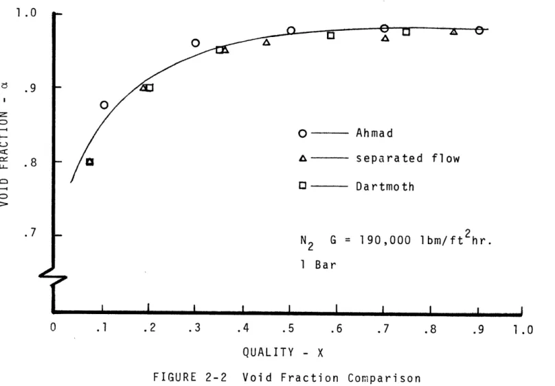
Ahmad [33] arrived at an expression for slip ratio based on void fraction data,

V Pk .205 - 0.016

S _{- = ~-}

2-4

V pf yP '

Void fractions calculated using this correlation agree favorably with those calculated using the Dartmouth corre-lation and the separated flow model presented in Wallis [34] for annular flow, Fig. 2-2.

3. Free Stream Weber Number - Droplet Break-Up. Droplets entrained by the vapor experience drag as the vapor velocity increases due to heat addition and evaporation. _{Equation (2-3) may again be used with Wec}

-6.5 and V _{equal to the free stream droplet velocity.} Whenever the relative velocity produces a Weber number

greater than 6.5, it is assumed that the droplet breaks up reducing We c _{stepwise, Fig. 2-lc. For analytical} pur-poses, we may hold the Weber number equal 6.5

and relate the drop diameter, D continuously with the relative velocity, (V - V )2

o

& - separated flow

D Dartmoth N2 G = 190,000 ibm/ft 2hr. 1 Bar I _I .1 .2 .3 .4 .5 .7 .8 .9 1.0 QUALITY - X

FIGURE 2-2 Void Fraction Comparison

1 .0

.9

4. Evaporation- Drop Size Decrease

Downstream of burnout, non-equilibrium may _{exist in the} flow, and heat can be transferred to the drops from super-heated vapor in addition to that from the hot wall to the drops. _{Thus, droplet size decreases due to evaporation.}

2.1.a _{Inverted Annular Flow}

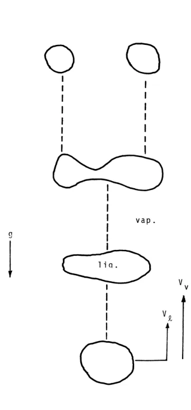
If the burnout quality is less than about 10%, the flow regime is normally inverted annular. Visual studies in the M.I.T. Heat Transfer Laboratory show that drops break from the liquid core with a size the scale of the core dia-meter. Baum [31] investigated heat transfer during inverted annular flow. _{From flow pattern maps developed by Hosler} [32], Baum concluded that inverted annular flow can exist only where void fractions are below 60%. Thus, initial drop sizes would be about 80% of tube diameter.

Figure 2-3 shows drop formation in inverted annular flow. The large drops formed from the liquid core break up because surface tension forces are not strong enough to keep the drop intact in the presence of high relative

velocities. A Weber number criterion should be important in determining initial drop size.

The definition of Weber number, Equation (2-3) can be combined with the definition of vapor and liquid

-39-2-3,a 2-3b cre vap. c

9

/U

velocities,

Vv

pyca

V 92-6

S

and the definition of void fraction 1

1

p 1

- X

P X

to yield an equation for drop diameter as a function of quality and free stream slip at burnout.

D pv a gc _Wec

-- =22 _2-8

DT G DT (S ~ l)2(pv

+(1

As the drops travel downstream, they experience in-creasing relative velocity due to evaporation in the flow. The free stream Weber number could again be exceeded,

and droplets would break up once more. Equation 2-8 could again be used to calculate a new drop diameter using local slip and quality (curve C, Fig. 2-3b).

-41-size (curve D, Fig. 2-3b) and no more break up occurs. This phenomenon is explained in more detail in section 2-lb under Annular Flow.

2,1 b Annular Flow

During annular flow, drops are formed at all points in the tube before burnout. Two types of sizing mechanisms may be important. The first is based on wave formation on

the liquid film due to Helmholtz instability.

Tatterson's analysis was for unheated annular flows where the vapor velocity remains constant throughout the tube. In heated annular flow, the vapor velocity is con-stantly changing and an average drop diameter can be

calcu-lated from Equation (2-1) using the local vapor velocity. Thus, the characteristic drop diameter will decrease as quality increases. Equation (2-1) can be rewritten in

terms of the quality and film slip using Equations (2-5) and (2-7),

D .106 C gc Pv 1/2 G DT 1 2-9

D D G2) v f + (1 - S )X

Thus, one characteristic drop size is associated with each point (or quality) before burnout.

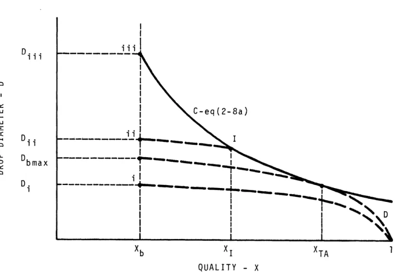
The variation of drop diameter due to Helmholtz instability, Equation (2-9) is shown sketched as a function of quality in Fig. 2-4 (curve A).

The film slip Weber number mechanism may also be im-portant in determining the size of drops originating from the liquid film. The critical Weber number, Equation (2-5) and definitions of liquid velocity, Equation (2-6) and void fraction (assuming a film slip determined void fraction), Equation (2-7) can again be combined using the film slip, Equation (2-4)

D pv a gc _Wec

DT G2 DT (S 1 2/ P + p ) ) 2 2-10 This is sketched as curve B in Fig. 2-4.

The free stream slip Weber number mechanism determines the droplet diameter due to increasing relative velocity caused by the accelerating vapor stream. The drop diameter as a

function of quality X and local free stream slip velocity is given by Equation (2-8) and is sketched as curve C on Fig. 2-4. Curve C lies above curve B because (V - V

)

Because non-equilibrium exists in the flow after burnout, the drops evaporate as they travel down the tube

Weber Number-Free Stream Slip (C)

---- Weber Number-Film Slip (B)

Helmhol tz Ins tability-Film Slip(A

--- Evaporation (D) C <rJ SIb Db B I 0TA it -F l Sl p A e TA _-. SI I 0 .1 Xb XTA 1.0 QUALITY - X

When the drop diameter gradient larger than the diameter gradie critical Weber number (the deri point TA of Fig. 2-4, brea evaporation alone determines dr the number of droplets in the f variation of drop diameter with can be determined using a mass

The liquid mass flow rate terms of the drop number flux,

42

nt due to the free stream vative of equation 2-8), k up no longer occurs and op size. After breakup ends,

low remains constant. The quality due to evaporation balance on the drops.

m can be defined in n ,

m = D3 _2-11

The definition of flowing quality,

X = 1 - m /m _2-12

can be combined with Equation (2-11) to give an equation for the quality in terms of drop diameter

3.

X = 1 - p₉nrD /6m

-45-D <. (1 - X) _2-13

and the drop diameter variation can be calculated.

D1

D 1 - X 3

._ =2-14

DTA _{I - TA}

This equation is curve D in Fig. 2-4, where

XTA and DTA are the quality and diameter at the tangent point of curves D and C (Equations (2-14) and (2-8))

Figure 2-5 is a plot of Equations (2-8), (2-9), (2-10), and (2-14) for Freon 12 (G = 486,940 lbm Q = 39371

Btu ~ft 2hr

Btu r . In this case, the gradient of the evaporation curve ft2hr

(Equation (2-14)) is greater than the gradient of the Weber number curve (Equation (2-8)) at burnout. Thus, no break-up would occur after the burnout point.

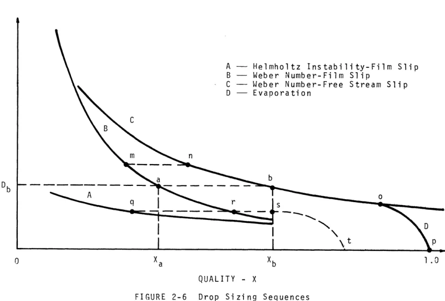
Figure 2-6 shows various sizing sequences a drop may undergo after initial formation.

Any drops formed during-annular flow larger than Db (Fig. 2-6), for example point m , follow a path n-n-b-o-p with no diameter change between m and n . Drops

formed with diameters smaller than Db , for example D9

70 X10~4

Weber no.- free stream slip; C

60 Weber no. - film slip; B

Helmholtz Instability; film slip; A Evaporation; D 4- 50 -Fr- 12 40 G = 486940 Q = 39371 30 uj c 20 _C 10 B 10 0 I I I .1 .2 .3 .4 .5 .6 .7 .8 .9 1 Xb QUALITY - X

A - Helmholtz Instability-Film Slip

B - Weber Number-Film Slip

C - Weber Number-Free Stream Slip

D - Evaporation LU C B m n b D b q r s

I

D

I

I

film slip criterion, remain at the initial diameter until they reach the burnout point, Xb . After burnout, they decrease in size due to evaporation, along paths q-r-s-t-or r-s-t

2.2 _{Average Drop Size at Burnout}

Most dispersed flow analyses use the concept of an average drop size to determine properties downstream of burnout. Drops are formed at points upstream of burnout, and the characteristic drop sizes are dependent on local conditions. _{It is necessary to find a method of averaging} these various drop sizes in order to facilitate dispersed flow heat transfer calculations.

2.2a _{Inverted Annular Flow}

Drops in inverted annular flow are formed after the burnout point. Initial average drop diameters for dispersed flow analyses should be based on the free stream Weber

number criterion, Equation (2-8), at the point of liquid core breakup, for example point C in Fig. 2-la.

2.2b Annular Flow

-49-drops formed upstream of burnout must be considered. All drops originating upstream of point a (Figure 2-6) form with initial drop diameter D > Db , due to Weber number

breakup from the film. As they travel downstream, they break up bythe freestream weber number criterion, to a

diameter Db at the burnout point. Those drops that form from curves B or A _{with initial diameters less than Db} remain at that size until they reach the burnout point. In order to determine the average drop size at burnout, the contribution of all of these drops must be considered. High speed photographic studies at the M.I.T. Heat Transfer Laboratory show that most entrained liquid forms from

pieces of liquid being thrown from the film. The local drop size would best be characterized by the film slip

Weber number mechanism. We therefore ignore the drop contri-bution from Helmholtz instability (Curve A, Fig. 2-6),

Eq. 2-9).

In order to compute average drop diameters at burnout, it is necessary to know the cumulative mass distribution, E at the burnout point with respect to quality. The cumula-tive distribution is that amount of mass entrained previous to a quality X which remains in the flow at burnout after accounting for deposition.

The mass entrained previous to point a (Fig. 2-6) which remains in the flow at burnout is E a All of this

mass can be characterized by a qualities X a and Xb, the entrai burnout, (Eb - Ea) will appear below Db as given by Equation ( average diameter is then

drop ned 1 at di 2-10) - _Xb D 1 D D dE

- = -

E

+

We assume that the mass cumulati varies linearly with quality, X from annular flow is assumed to begin (thi sed more fully in Appendix A-5).

diameter Db. Between iquid remaining at ameters decreasing

The mass weighted

dX] 2-15 ve distribution, E E=0 at X=0.l where s assumption is discus-E X - 0.1 Eb Xb ~ 0.1 2-16 Equation (2-15) becomes D DT X Xa _{- 0.1 Db b} Xb _{- 0.1 DT} X

x

- and integrating, the average DT determined. dX Xb - 0.1 into drop Equation(2-17) for diameter can be 2-17

-51-D 1 Db P 2 We v 4 gc

DT

Xb

~

0.1

DT

Xa

_(Vi

_(Sf

_{_}

₂

_G

_DT

S1

12-18

(v vflbv

a

vb

Sf

(P

v

-f

DTcan be calculated using Equation (2-8) evaluated at burnout conditions.

The quality, X a where the film slip drop diameter equals the free stream slip drop diameter at burnout (Db) is obtained by equating drop diameters from Equations

(2-6) and (2-8).

S+ )X S - 1

--

)

=

2-19

+ pI- S

If

x

CHAPTER III

DISPERSED FLOW HEAT TRANSFER MODEL 3.1 Formulation

The dispersed flow consists of three of the Fig. 3-1. A sma

vapor travelling ling with axial velocity gradien toward the wall are high enough droplets ride on tion. The kinet drop deformation 11 portion v t t i

heat transfer model L1,2,3,5,18] heat transfer mechanisms shown i

of the tube wall is shown with with velocity V v an

elocity V 9 . Becaus

s in the flow, the en ith velocity Vp . W

o prevent drop wettin a vapor layer produce c energy of the drop and stored as surface

d e t a g d i droplets travel-of turbulence and rained drops move 11 temperatures

, and approaching by rapid evapora-s abevapora-sorbed by energy. Surface forces try to restore the drop to a

the drop rebounds from the wall and Four heat transfer mechanisms from this representation.

spherical shape, and travels downstream. can be identified

1. Heat transfer directly from the wall to the vapor - Qw'v _'

\

\

\

\~\

\ \

Q" II

Qc

FIGURE 3-1 Heat Transfer Mechanisms in Dispersed

V V wv 0 Flow

Q It

2. Heat Transfer from the Vapor to the Entrained Droplets - QvD

Non equilibrium exists in the flow, and super-heated vapor transfers heat to the drops.

3. Heat Dropl lish the the local

Transfer from the Wall ets in close proximity local temperature profi

heat transfer.

to to le,

the Drops -

QwD

the wall estab-and therefore

Included not contained

this analysis is one additional mechanism previous analyses.

4. Heat Transfer by Axial Conduction in the Tube - Qc' High temperature gradients can exist in the tube wall near burnout and axial conduction could be

impor-tant.

The emphasis of this chapter is to develop a mech-anistic heat transfer model which can predict tube wall temperatures in constant heat flux dispersed upflow.

-55-ASSUMPTIONS

Several assumptions are made which simplify the heat transfer model. These assumptions and their reasoning follow:

1. The Flow is Steady State

Solution schemes have been compared to steady state experimental data. In some real world cases, this is a good approximation. For example, a once through steam generator operating under constant power condi-tions would be essentially a steady state process. Other cases might not be steady state, however, could

be considered "quasi" steady state. During the re-flood portion of a nuclear reactor loss of coolant accident, cold water is used to cool fuel rods which are well above the Leidenfrost temperature. In this case, the burnout point or quench front velocities are on the order of inches per minute, and "quasi" steady state analysis should be appropriate. In other cases, where quench fronts move faster, as might occur in quench cooling of metals, the steady state assumption would not be appropriate, and a modification of this

2. The System is under Constant Heat Flux Conditions.

3. Equilibrium Quality Exists at Burnout.

Before the burnout point, vapor generated at the wall must travel through the liquid film, and little vapor

superheat could exist . Therefore, the vapor and liquid temperatures must be equal at burnout.

4 out and pletely

. The liquid is at saturation temperature at burn-remains at the saturation temperature until com-evaporated.

5. The Drop Size Distribution can be Characterized by One Average Drop Size.

Drops of many sizes are present in dispersed flow. The assumption of a single drop size in the flow will cause a slight overprediction of equilibrium near actual

qualities of 1 , since drops larger than the average drop

size will exist in the flow, and will take longer to evaporate than a drop of average size.

Over the major portion of the flow pattern, the as-sumption of a single drop size would have little effect on the calculated wall temperatures, since the number of very large droplets existing in the flow is very small.

-57-6. The Wall Temperature at the Dryout Point is the Homogeneous Nucleation Temperature. A liquid spontaneously boils at the homogeneous nucleation temperature. Any surface with temperature greater than the homogeneous nucleation temperature would prevent wetting. Previous to the burnout point, the liquid on the wall is in transition boiling. Once dryout occurs, liquid can no longer wet the wall. At this point, the wall temperature is thus assumed to be at the homogeneous

nucleation temperature.

7. Liquid and Vapor Velocities are Uniform Across the Tube.

The vapor flow regimes present are turbulent, and vapor velocities would be nearly uniform. As stated earlier, experimental evidence shows that liquid drop velocities are approximately uniform across the tube and

KNOWNS AND UNKNOWNS Knowns: Xb -G -Q" -Fluid Properties Tube Properties a burnout quality mass flux heat flux nd Dimensions Unknowns: Initial Co D -0 S-ndi tions drop diameter slip

Local Condi tions

X -D -V -T -

Tw-V, , V

and

a

calculated from Equations (2-5),(2-6) known.

-59-The model begins at burnout, where initial drop size is calculated by the procedure outlined in Chapter II, and the liquid velocity is calculated using the droplet momen-tum equation. The solution proceeds downstream using gradients of droplet diameter, actual quality, liquid velocity, vapor temperature, and an algebraic energy bal-ance at the wall. Correlations are used for droplet heat transfer coefficient, droplet drag coefficient, and heat transfer coefficient between the wall and vapor. An analytic model is used to determine wall to droplet heat transfer.

3.la Dryout Conditions

The droplet momentum equation can be solved for free stream slip ratio at burnout, once the liquid accelera-tion is known. The liquid acceleraaccelera-tion at burnout

dV dz

can be rewritten using the definition of liquid velocity Equation (2-6).

dVi, V d d z G d -V k- --a s

p-

dz

Under dispersed flow conditions, void fractions slightly less than one increase with distance while slip ratios, slightly greater than one decrease with distance.

There-1 d X

dso 1 X q

fore, at burnout, we assume that X s

-eq d z ct s d z (see Appendix A-1 ).

The equilibrium quality at any point in the tube is,

3-2 X Q(4Q(z + Zb

GhfgD _T

differentiating and substituting into Equation (3-1) with Xq d(s-) dXe ' eq dz 'st d z dz 1 d z s Ot The droplet acceleration, the the drop. 4 QD p vh f gD T

momentum equation consists of force due to gravity, and the

dropl et drag on

Acceleration dV 7

D3

T D2 2

(p9 - pv ) + - _{C D P v 9} 8

-1) 2 3-4

on (3-3) for dV _dz9 and the definition Equation (2-6), results in an equation slip _ratio. 1 +/1 4 3 - (1 p p~g(1 - D"1-a2 G2 CD D -G CD X / 4 p p g 1 - 2 3 D a- 2 3 G2 CD X2 16 Q'" D 3 Gh D

The definition of void fraction, Equation (2-7) the free stream Weber number criterion, Equation (2-8) be combined with Equation (3-5) in an iterative soluti

to solve for slip, void fraction and drop diameter at out. 3-5 and can on . burn-3.lb Governing Equations

When modeling two phase flow, transport equations must be written for both phases. A set of equations which describe dispersed flow have been used by several

investigators [1-3,5]. A good review of dispersed flow -61-Gravity 7r D 6 Drag

(1

transport equations is given by Crowe [36J.

The equations presented here are those used by Forslund [3], Plummer [18] and Groeneveld [5].

1. Liquid Velocity Gradient

The droplet momentum balance Equation(3-4) presented in section 3-la is rewritten here

dV dz g p 3 p

1

_-CD

_Dv+

_V(s

where CD is the droplet drag coefficient.

2. Droplet Diameter Gradient

The liquid mass decreases due to droplet evaporation. An energy balance on the liquid includes heat transferred

tI

to the liquid from the superheated vapor - vD and heat

transferred from the wall to the liquid -

Q

This in turn determines the rate of liquid mass decrease.

h -m9 _{Q 'D + Q wD}

d

t

i

where _{m ,}

_Q'vD'

_D

, are per

of change

unit length of tube. dm,

-63-distance down the tube.

dm dma9

dt dz 3-7

For a unit length of tube, the relationship between the liquid mass and the drop diameter is:

7T D3 T T2

m = n p 3-8

6 4

where n is the number of drops per unit volume. Or, using Equations (3-7) and (3-8) and a constant drop number

over dz ,

dm 1 2 2 2 dD

- - V n p 9 DT D

dt 8 d z

3-9

VAPOR TO DROP HEAT TRANSFER - QD

The heat transfer from the vapor to a single drop-let is:

(T - Ts) ₃

qvD _{- ' D2}

hD

The heat transfer to all (again for a unit length

entrained droplets becomes: of tube) , DT2

QvD

QvD

D

hD

Ts) n

WALL TO DROP HEAT TRANSFER -

QD

The heat transfer from the wall to a single droplet is:

T[ D3

q wD o k h f 3-12

where the effectiveness, e is defined as the heat transfer to the drop divided by the total amount of heat needed to completely evaporate the drop.

The liquid mass flux toward the wall per length of tube is:

-65-m=

2 VP rDT (1 - c:)

assuming half of the liquid is travelling toward with velocity V and half is travelling away from

The drop deposition rate (#/hr ft) is iip by the mass per drop.

however, (1

6

ip

3

VP

DT

(1

- a)

The wall to drop heat transfer is the product of the num-ber of drops impacting per unit time and the heat trans-fer per impact. Combining Equations (3-12), (3-14) and (3-15)

, v2 D3 DT

wD = 12 hfg Vp p Yn e 3-16

Placing Equations (3-9), (3-lla) and (3-16) into Equation (3-6) 3-13

dD h (T -T ) - = -2 [Dv s+

dz _{-V 91pz h f}

3. Actual Quality The liquid flux,

1

D V

]

3 D T V 9

Gradient

G(l - X) can be written in terms of the axial droplet flux, n

G(l - X) - 3 r

D

is the number of drops passing a cross section time.

Differentiating with respect to z and assuming droplet flux is uniform across an element

P G

2 d z G 7T D T _{d z} back substituting Equation (3-18) for

dx 3(1 - x) dD

4. Vapor Temperature

D dz

Gradient

The enthalpy increase in the vapor is the differ-ence between total heat flux into the fluid minus that used

to evaporate the liquid.

3-17 TrDT 2 3-18 the V 9 n n D2 dz dDl 3-19 3-20

-67-Qy= QT ~

VAPOR ENTHALPY INCREASE: _Q

The vapor enthalpy increase across an element dz is:

2 = IdT

Qv

4 Pdz

The total heat transferred into the system is:

QT= Q 7r DT

LIQUID EVAPORATION: Q

The heat needed to evaporate the resulting vapor to free stream

3-23

the liquid and raise temperature is:

I dx

Q =

4 Tdz

combining Equations (3-21) through (3-24),

3-24 3-21

dT 4

Q"

dz _D TG _{X C}

5. Energy Bal The heat into impacting the wall

h f

gf dX

VAPOR HEAT TRANSFER: Heat transfer to the

at the Wall

luid must all go into the or into the vapor Qwy

QI' wv

vapor/unit length:

QWV

where _{h is the wall to vapor heat transfer coefficient,} and a is the void fraction which approximates the frac-tion of wall area free of drop interacfrac-tion.

WALL TO DROP HEAT TRANSFER: Q _wD'

QwD is obtained is obtained by combining Equations (3-15) and (3-16) 3-27 -wD = (1 - a)T DT hfg V p % 3-25 drops

-69-A non-linear temperature profile may exist under the drop, i.e. some heat from the wall may be used to super-heat the vapor evaporated from the drop as well as evapo-rate the drop itself. A factor 1 is included in the

2

analysis to account for a non-linear temperature profile beneath the drop.

Thus, combining Equations (3-26) and (3-27) with the total energy into the system Q , Equation (3-23) and

a2 Q" 1 (1 _{a) h f V pYI} T -_w T 1 ( - P 3-28 v _{2 hw} w ~ w2 3-lc Correlations

Droplets in dispersed flow are exposed to an environ-ment which may alter both the heat transfer and drag

char-acteristics from that expected for simpler flows. Some of the more important effects are discussed below.

1. Droplet Heat Transfer Coefficient - Eq. (3-lla) Droplet heat transfer coefficients may be affected by evaporation or free stream turbulence.

EFFECT OF EVAPORATION

Mass transfer away from the drop has been found to decrease the heat transfer. Empirical shielding factors have been used to account for this effect. One common form which has been used by Ross et al [37] and Yuen et al [38] is:

NuD(1 + CB)n = Nu _3-29

where Nu0 is the Nusselt number for zero mass transfer, and B is the Spalding transport, or mass transfer

number,

Cp(T - Ts 3

B = 3-30

h _hfg -g R/*_m

q R is the radiative heat exchange, which was

present in their experiment, and m is the mass transfer rate from the drop.

Ross experimentally investigated water drops

evaporating in a steam environrent. Drop Reynolds num-bers were in the range of 30 - 200 and the empirical shielding function which gave a satisfactory fit was

-71-The zero mass transfer Nusselt number which Ross used was:

Nu1=2 + .369 Pr 1/3 Re.5 8

Yuen and Chen [38] chose the form

a shielding function in

NuD _{(1 + B) =}

Nu₀

to fit data of water and m drop Reynolds numbers from stream temperatures (qR/m as it had little effect on Yuen and Chen used the Ran the zero mass transfer Nus

ethanol evaporating in air for 200 - 1000 and various free was neglected in their analysis

the overall heat transfer). z and Marshall correlation as selt number.

Nu = 2 + .6 Re 1/2 Pr 1/3

0 f f

Because the drop Reynolds and Chen were closer to th

numbers e range investigated by Yuen encountered in this analysis, and (Appendix A-2) radi ation , Yuen's s

to the drops is negligable hielding function

3-31

C (T - T

)

fg

and zero mass transfer number Equation (3-32) were chosen for use in Equation (3-31)

EFFECT OF FREE STREAM TURBULENCE

Drop heat transfer and drag correlations are based on the relative velocity between the drop and vapor. Drop Reynolds numbers in this study were found to be in the range where the boundary layer is laminar (Z 100 < Re < 1000). However, the free stream is turbulent, and turbulent fluctuations are present.

Hayward and Pei

L43J

D a function of position on the sphere), showed a dependence on the turbulence level in the flow, however, the

over-all Nusselt numbers were correlated well by solid sphere correlations. Reynolds numbers varied from 2500 to 6500 and turbulence intensity from .5% to 5.7%.

Maisel and Sherwood [45] studied the effect of free stream turbulence on mass transfer coefficients for

73-spheres. Their experimental coefficients incre

bers and also with ever, low Reynolds lence levels had 1 ficient. They al turbulence in the

Turbulence 1 tween the droplets in dispersed flow. data shows little at a sphere Reyn

Typical drop range from 10 to 1 therefore free str effect on the heat

The heat tra that suggested by

results show mass asing with increasing s

increasing turbulence numbers in combination ittle effect on the mas so found no effect due flow.

evels based on the rela and vapor are approxim

For a turbulence leve increase in the mass tr

transfer phere Reynolds n intensity.

How-with low turbu-s tranturbu-sfer coef-to the scale of

um-tive velocity be-ately 10% - 20% 1 of 20%, Maisel's ansfer coefficient olds number of 2550.

Reynolds numbers in dispersed flow 000 over the major portion of the flow, eam turbulence is expected to have little

transfer characteristics.

nsfer coefficient used in this study is Yuen, Equations(3-31) and (3-32)