https://doi.org/10.4224/5763652
READ THESE TERMS AND CONDITIONS CAREFULLY BEFORE USING THIS WEBSITE. https://nrc-publications.canada.ca/eng/copyright
Vous avez des questions? Nous pouvons vous aider. Pour communiquer directement avec un auteur, consultez la première page de la revue dans laquelle son article a été publié afin de trouver ses coordonnées. Si vous n’arrivez pas à les repérer, communiquez avec nous à PublicationsArchive-ArchivesPublications@nrc-cnrc.gc.ca.
Questions? Contact the NRC Publications Archive team at
PublicationsArchive-ArchivesPublications@nrc-cnrc.gc.ca. If you wish to email the authors directly, please see the first page of the publication for their contact information.
Archives des publications du CNRC
For the publisher’s version, please access the DOI link below./ Pour consulter la version de l’éditeur, utilisez le lien DOI ci-dessous.
Access and use of this website and the material on it are subject to the Terms and Conditions set forth at
Human-Level Performance on Word Analogy Questions by Latent
Relational Analysis
Turney, Peter
https://publications-cnrc.canada.ca/fra/droits
L’accès à ce site Web et l’utilisation de son contenu sont assujettis aux conditions présentées dans le site LISEZ CES CONDITIONS ATTENTIVEMENT AVANT D’UTILISER CE SITE WEB.
NRC Publications Record / Notice d'Archives des publications de CNRC:
https://nrc-publications.canada.ca/eng/view/object/?id=9179349a-ad7e-4326-85d3-72dd85f95e6a https://publications-cnrc.canada.ca/fra/voir/objet/?id=9179349a-ad7e-4326-85d3-72dd85f95e6a
Institute for
Information Technology
Institut de technologie de l'information
Human-Level Performance on Word Analogy
Questions by Latent Relational Analysis *
Turney, P.
December 2004
* published as NRC/ERB-1118. December 6, 2004. 32 Pages. NRC 47422.
Copyright 2004 by
National Research Council of Canada
Permission is granted to quote short excerpts and to reproduce figures and tables from this report, provided that the source of such material is fully acknowledged.
Institute for
Information Technology
Institut de technologie de l'information
H um a n-Le ve l Pe rform a nc e
on Word Ana logy Que st ions
by La t e nt Re la t iona l Ana lysis
Turney, P.
December 2004
Copyright 2004 by
National Research Council of Canada
Permission is granted to quote short excerpts and to reproduce figures and tables from this report, provided that the source of such material is fully acknowledged.
Human-Level Performance on Word Analogy Questions
by Latent Relational Analysis
Abstract... 3
1 Introduction ... 3
2 Applications for Measures of Relational Similarity ... 6
3 Related Work ... 10
4 Latent Relational Analysis ... 12
5 Experiments with Word Analogy Questions ... 19
5.1 Baseline LRA System ... 19
5.2 LRA versus VSM and PRMC ... 20
5.3 Human Performance... 22
5.4 Varying the Number of Dimensions in SVD ... 22
5.5 LRA without SVD... 22
5.6 LRA without Synonyms... 23
5.7 LRA without Synonyms and without SVD ... 23
6 Experiments with Noun-Modifier Relations ... 23
6.1 Baseline LRA with Single Nearest Neighbour ... 24
6.2 LRA versus VSM ... 24
7 Discussion... 25
8 Conclusion ... 26
Acknowledgements ... 27
Human-Level Performance on Word Analogy Questions
by Latent Relational Analysis
Abstract
This paper introduces Latent Relational Analysis (LRA), a method for measuring relational similarity. LRA has potential applications in many areas, including information extraction, word sense disambiguation, machine translation, and information retrieval. Relational similarity is correspondence between relations, in contrast with attributional similarity, which is correspondence between attributes. When two words have a high degree of attributional similarity, we call them synonyms. When two pairs of words have a high degree of relational similarity, we say that their relations are analogous. For example, the word pair mason/stone is analogous to the pair carpenter/wood; the relations between mason and stone are highly similar to the relations between carpenter and wood. Past work on semantic similarity measures has mainly been concerned with attributional similarity. For instance, Latent Semantic Analysis (LSA) can measure the degree of similarity between two words, but not between two relations. Recently the Vector Space Model (VSM) of information retrieval has been adapted to the task of measuring relational similarity, achieving a score of 47% on a collection of 374 college-level multiple-choice word analogy questions. In the VSM approach, the relation between a pair of words is characterized by a vector of frequencies of predefined patterns in a large corpus. LRA extends the VSM approach in three ways: (1) the patterns are derived automatically from the corpus (they are not predefined), (2) the Singular Value Decomposition (SVD) is used to smooth the frequency data (it is also used this way in LSA), and (3) automatically generated synonyms are used to explore reformulations of the word pairs. LRA achieves 56% on the 374 analogy questions, statistically equivalent to the average human score of 57%. On the related problem of classifying noun-modifier relations, LRA achieves similar gains over the VSM, while using a smaller corpus.
1 Introduction
There are (at least) two kinds of semantic similarity. Relational similarity is correspondence between relations, whereas attributional similarity is correspondence between attributes (Medin et al., 1990, 1993). Many algorithms have been proposed for measuring the attributional similarity between two words (Lesk, 1969; Church and Hanks, 1989; Ruge, 1992; Dunning, 1993; Smadja, 1993; Resnik, 1995; Landauer and Dumais, 1997; Jiang and Conrath, 1997; Lin, 1998a; Turney, 2001; Budanitsky and Hirst, 2001; Pantel and Lin, 2002; Banerjee and Pedersen, 2003). When two words have a high degree of attributional similarity, we call them synonyms. Applications for measures of attributional similarity include the following:
• recognizing synonyms (Landauer and Dumais, 1997; Turney, 2001; Jarmasz and
Szpakowicz, 2003; Terra and Clarke, 2003; Turney et al., 2003)
• information retrieval (Deerwester et al., 1990; Dumais, 1993; Hofmann, 1999)
• determining semantic orientation, criticism versus praise (Turney, 2002; Turney and
Littman, 2003a)
• measuring textual cohesion (Morris and Hirst, 1991; Barzilay and Elhadad 1997; Foltz et al., 1998; Turney, 2003)
• automatic thesaurus generation (Ruge, 1997; Lin, 1998b; Pantel and Lin, 2002)
• word sense disambiguation (Lesk, 1986; Banerjee and Pedersen, 2003; Patwardhan
et al., 2003; Turney, 2004)
Recently, algorithms have been proposed for measuring relational similarity; that is, the semantic similarity between two pairs of words (Turney et al., 2003; Turney and Littman, 2003b, 2005). When two word pairs have a high degree of relational similarity, we say they are analogous. For example, the pair traffic/street is analogous to the pair water/riverbed. Traffic flows over a street; water flows over a riverbed. A street carries traffic; a riverbed carries water. The relations between traffic and street are similar to the relations between water and riverbed. In fact, this analogy is the basis of several mathematical theories of traffic flow (Daganzo, 1994; Zhang, 2003; Yi et al., 2003). Applications for measures of relational similarity include the following:
• recognizing word analogies (Turney et al., 2003; Turney and Littman, 2003b, 2005)
• classifying semantic relations (Rosario and Hearst, 2001; Rosario et al., 2002;
Nastase and Szpakowicz, 2003; Turney and Littman, 2003b, 2005)
• machine translation
• word sense disambiguation
• information extraction (Paice and Black, 2003)
• automatic thesaurus generation (Hearst, 1992a; Berland and Charniak, 1999)
• information retrieval (Hearst, 1992b)
• processing metaphorical text (Martin, 1992; Dolan, 1995)
• identifying semantic roles (Gildea and Jurafsky, 2002)
• analogy-making (Gentner, 1983; Falkenhainer et al., 1989; Falkenhainer, 1990)
Since measures of relational similarity are not as well developed as measures of attributional similarity, the applications of relational similarity (both actual and potential) are not as well known. Section 2 briefly outlines how a measure of relational similarity may be used in the above applications.
We discuss past work on relational similarity and related problems in Section 3. Our work is most closely related to the approach of Turney and Littman (2003b, 2005), which adapts the Vector Space Model (VSM) of information retrieval to the task of measuring relational similarity. In the VSM, documents and queries are represented as vectors, with dimensions corresponding to the words that appear in the given set of documents (Salton and McGill, 1983; Salton and Buckley, 1988; Salton, 1989). The value of an element in a vector is based on the frequency of the corresponding word in the document or query. The similarity between a document and a query is typically measured by the cosine of the angle between the document vector and the query vector (Baeza-Yates and Ribeiro-Neto,1999). Similarly, Turney and Littman (2003b, 2005) represent the semantic relations between a pair of words (e.g., traffic/street) as a vector in which the elements are based on the frequency (in a large corpus) of patterns that connect the pair (e.g., “traffic in the street”, “street with traffic”). The relational similarity
between two pairs (e.g., traffic/street and water/riverbed) is then measured by the cosine of the angle between their corresponding vectors.
In Section 4, we introduce an algorithm for measuring relational similarity, which we call Latent Relational Analysis (LRA). The algorithm learns from a large corpus of unlabeled, unstructured text, without supervision. LRA extends the VSM approach of Turney and Littman (2003b, 2005) in three ways. Firstly, the connecting patterns are derived automatically from the corpus. Turney and Littman (2003b, 2005), on the other hand, used a fixed set of 64 manually generated patterns (e.g., “… in the …”, “… with …”). Secondly, Singular Value Decomposition (SVD) is used to smooth the frequency data. SVD is also part of Latent Semantic Analysis (LSA), which is commonly used for measuring attributional similarity (Deerwester et al., 1990; Dumais, 1993; Landauer and Dumais, 1997). Thirdly, given a word pair such as traffic/street, LRA considers transformations of the word pair, generated by replacing one of the words by synonyms, such as traffic/road, traffic/highway. The synonyms are taken from Lin’s (1998b) automatically generated thesaurus.
Measures of attributional similarity have become a popular application for electronic thesauri, such as WordNet and Roget’s Thesaurus (Resnik, 1995; Jiang and Conrath, 1997; Budanitsky and Hirst, 2001; Banerjee and Pedersen, 2003; Patwardhan et al., 2003; Jarmasz and Szpakowicz 2003). Recent work suggests that it is possible to use WordNet to measure relational similarity (Veale, 2003). We expect that this will eventually become another common application for electronic thesauri. There is evidence that a hybrid approach, combining corpus-based relational similarity with thesauri-based relational similarity, will prove to be superior to a purebred approach (Turney et al., 2003). However, the scope of the current paper is limited to empirical evaluation of LRA, a purely corpus-based approach.
Section 5 presents our experimental evaluation of LRA with a collection of 374
multiple-choice word analogy questions from the SAT college entrance exam.1 Table 1 shows a
typical SAT question. In the educational testing literature, the first pair (mason:stone) is called the stem of the analogy. We use LRA to calculate the relational similarity between the stem and each choice. The choice with the highest relational similarity to the stem is output as the best guess.
Table 1. A sample SAT question.
Stem: mason:stone (a) teacher:chalk (b) carpenter:wood (c) soldier:gun (d) photograph:camera Choices: (e) book:word Solution: (b) carpenter:wood
The average performance of college-bound senior high school students on verbal SAT questions in 2002 (approximately the time when the 374 questions were collected) corresponds to an accuracy of about 57% (Turney and Littman, 2003b, 2005). LRA achieves an accuracy of about 56%. On these same questions, the VSM attained 47%.
1
The College Board has announced that analogies will be eliminated from the SAT in 2005, as part of a shift in the exam to reflect changes in the curriculum.
One application for relational similarity is classifying semantic relations in noun-modifier pairs (Nastase and Szpakowicz, 2003; Turney and Littman, 2003b, 2005). In Section 6, we evaluate the performance of LRA with a set of 600 noun-modifier pairs from Nastase and Szpakowicz (2003). The problem is to classify a noun-modifier pair, such as “laser printer”, according to the semantic relation between the head noun (printer) and the modifier (laser). The 600 pairs have been manually labeled with 30 classes of semantic relations. For example, “laser printer” is classified as instrument; the printer uses the laser as an instrument for printing. The 30 classes have been manually organized into five general types of semantic relations.
We approach the task of classifying semantic relations in noun-modifier pairs as a supervised learning problem. The 600 pairs are divided into training and testing sets and a testing pair is classified according to the label of its single nearest neighbour in the training set. LRA is used to measure distance (i.e., similarity, nearness). LRA achieves an accuracy of 39.8% on the 30-class problem and 58.0% on the 5-class problem. On the same 600 noun-modifier pairs, the VSM had accuracies of 27.8% (30-class) and 45.7% (Turney and Littman, 2003b, 2005).
We discuss the experimental results, limitations of LRA, and future work in Section 7 and we conclude in Section 8.
2 Applications for Measures of Relational Similarity
This section sketches some applications for measures of relational similarity. The following tasks have already been attempted, with varying degrees of success, by researchers who do not explicitly consider relational similarity; only a few of the applications have been framed as involving relational similarity. It is outside the scope of this paper to demonstrate that explicitly considering relational similarity will yield improved performance on all of these various tasks. Our intent in this section is only to suggest that the tasks can be cast in terms of relational similarity.
Recognizing word analogies: The problem is, given a stem word pair and a finite list of
choice word pairs, select the choice that is most analogous to the stem. This problem was first attempted by a system called Argus (Reitman, 1965), using a small hand-built semantic network. Argus could only solve the limited set of analogy questions that its programmer had anticipated. Argus was based on a spreading activation model and did not explicitly attempt to measure relational similarity. As mentioned in the introduction, Turney and Littman (2003b, 2005) adapt the VSM to measure relational similarity and evaluate the measure using SAT analogy questions. We follow the same approach here. This is discussed in detail in Sections 3 and 5.
Classifying semantic relations: The task is to classify the relation between a pair of words. Often the pairs are restricted to noun-modifier pairs, but there are many interesting relations, such as antonymy, that do not occur in noun-modifier pairs. Rosario and Hearst (2001) and Rosario et al. (2002) classify noun-modifier relations in the medical domain, using MeSH (Medical Subject Headings) and UMLS (Unified Medical Language System) as lexical resources for representing each noun-modifier pair with a feature vector. They trained a neural network to distinguish 13 classes of semantic relations. Nastase and Szpakowicz (2003) explore a similar approach to classifying general noun-modifier pairs (i.e., not restricted to a particular domain, such as medicine), using WordNet and Roget’s Thesaurus as lexical resources. Vanderwende (1994) used hand-built rules, together with a lexical knowledge base, to classify noun-modifier pairs. None of these approaches explicitly involved measuring relational similarity, but any
classification of semantic relations necessarily employs some implicit notion of relational similarity, since members of the same class must be relationally similar to some extent. Barker and Szpakowicz (1998) tried a corpus-based approach that explicitly used a measure of relational similarity, but their measure was based on literal matching, which limited its ability to generalize. Turney and Littman (2003b, 2005) used the VSM to measure relational similarity as a component of a single nearest neighbour algorithm. We take the same approach here, substituting LRA for the VSM, in Section 6.
Machine translation: Noun-modifier pairs are extremely common in English. For
instance, WordNet 2.0 contains more than 26,000 noun-modifier pairs, yet many common noun-modifiers are not in WordNet, especially technical terms. Machine translation cannot rely primarily on manually constructed translation dictionaries for translating noun-modifier pairs, since such dictionaries are necessarily very incomplete. It should be easier to automatically translate noun-modifier pairs when they are first classified by their semantic relations. Consider the pair “electron microscope”. Is the semantic relation purpose (a microscope for viewing electrons), instrument (a
microscope that uses electrons), or material (a microscope made of electrons)?2 The
answer to this question should facilitate translation of the individual words, “microscope” and “electron”, and may also help to determine how the individual words are to be combined in the target language (e.g., what order to put them in, what suffixes to add, what prepositions to add). One possibility would be to reformulate noun-modifier pairs as longer phrases, in the source language, before machine translation. After the semantic relations have been identified, a set of templates can be used to reformulate the noun-modifier pairs. For example, “If ‘A B’ is classified as instrument, reformulate it as ‘B that uses A’.”
Word sense disambiguation: Noun-modifier pairs are almost always monosemous
(Yarowsky, 1993, 1995). We hypothesize that the implicit semantic relation between the two words in the pair narrowly constrains the possible senses of the words. More generally, we conjecture that the intended sense of a word is determined by its semantic relations with the other words in the surrounding text. If we can identify the semantic relations between the given word and its context, then we can disambiguate the given word. Consider the noun-modifier pair “plant food”. In isolation, “plant” could refer to an industrial plant or a living organism. Once we have determined that the implicit semantic relation in “plant food” is beneficiary (the plant benefits from the food), as opposed to, say, location at (the food is located at the plant), the sense of “plant” is constrained to
“living organism”.3 As far as we know, no existing word sense disambiguation system
makes explicit use of a measure of relational similarity, but we believe this is a promising approach to word sense disambiguation.
Information extraction: Paice and Black (2003) describe a system that identifies the
key terms in a document and then discovers the semantic relations between the key terms. For example, from a document entitled Soil Temperature and Water Content, Seeding Depth, and Simulated Rainfall Effects on Winter Wheat Emergence, they were able to automatically extract the terms “seeding depth”, “emergence”, and “winter wheat”, and then discover the semantic relations among these three terms. Their corpus consisted of papers on agriculture (crop husbandry) and their algorithm is limited to relations among influences (e.g., seeding depth), properties (e.g., emergence), and
2
These three semantic relations are from the 30 classes of Nastase and Szpakowicz (2003). 3
objects (e.g., winter wheat). They used manually generated rules to identify the semantic relations, but an alternative approach would be to use supervised learning, which would make it easier to expand the system to a wider range of documents and a larger set of semantic relations. For example, a measure of relational similarity could be used as a distance measure in a nearest neighbour algorithm (Turney and Littman, 2003b, 2005).
Automatic thesaurus generation: Hearst (1992a) presents an algorithm for learning
hyponym (type of) relations from a corpus and Berland and Charniak (1999) describe how to learn meronym (part of) relations from a corpus. These algorithms could be used to automatically generate a thesaurus or dictionary, but we would like to handle more relations than hyponymy and meronymy. WordNet distinguishes more than a dozen semantic relations between words (Fellbaum, 1998) and Nastase and Szpakowicz (2003) list 30 semantic relations for noun-modifier pairs. Hearst (1992a) and Berland and Charniak (1999) use manually generated rules to mine text for semantic relations. Turney and Littman (2003b, 2005) also use a manually generated set of 64 patterns. LRA does not use a predefined set of patterns; it learns patterns from a large corpus. Instead of manually generating new rules or patterns for each new semantic relation, it is possible to automatically learn a measure of relational similarity that can handle arbitrary semantic relations. A nearest neighbour algorithm can then use this relational similarity measure to learn to classify according to any given set of classes of relations.
Information retrieval: Current search engines are based on attributional similarity; the
similarity of a query to a document depends on correspondence between the attributes of the query and the attributes of the documents (Baeza-Yates and Ribeiro-Neto,1999). Typically the correspondence is exact matching of words or root words. Latent Semantic Indexing allows more flexible matching, but it is still based on attributional similarity (Deerwester et al., 1990; Dumais, 1993). Hearst (1992b) outlines an algorithm for recognizing text in which an agent enables or blocks an event. The algorithm was designed for use in information retrieval applications, but it has not yet been implemented. If we could reliably classify semantic relations, then we could ask new kinds of search queries:
• find all documents about things that have been enabled by the Canadian government
• find all documents about things that have a causal relation with cancer
• find all documents about things that have an instrument relation with printing
Existing search engines cannot recognize the implicit instrument relation in “laser printer”, so the query “instrument and printing” will miss many relevant documents. A measure of relational similarity could be used as a component in a supervised learning system that learns to identify semantic relations between words in documents. These semantic relations could then be added to the index of a conventional (attributional) search engine. Alternatively, a search engine could compare a query to a document using a similarity measure that takes into account both relational similarity and attributional similarity. A query might be phrased as a word analogy problem:
• find all documents about things that are to printers as lasers are to printers
• find all documents about things that are to dogs as catnip is to cats
• find all documents about things that are to Windows as grep is to Unix
Processing metaphorical text: Metaphorical language is very common in our daily life;
Martin (1992) notes that even technical dialogue, such as computer users asking for help, is often metaphorical:
• How can I kill a process?
• How can I get into the LISP interpreter?
• Tell me how to get out of Emacs.
Human-computer dialogue systems are currently limited to very simple, literal language. We believe that the task of mapping metaphorical language to more literal language can be approached as a kind of word analogy problem:
• kill is to an organism as stop is to a process
• get into is to a container as start is to the LISP interpreter
• get out of is to a container as stop is to the Emacs editor
We conjecture that a measure of relational similarity can be used to solve these kinds of word analogy problems, and thus facilitate computer processing of metaphorical text. Gentner et al. (2001) argue that novel metaphors are understood using analogy, but conventional metaphors are simply recalled from memory. A conventional metaphor is a metaphor that has become entrenched in our language (Lakoff and Johnson, 1980). Dolan (1995) describes an algorithm that can recognize conventional metaphors, but is not suited to novel metaphors. This suggests that it may be fruitful to combine Dolan’s (1995) algorithm for handling conventional metaphorical language with an algorithm such as LRA for handling novel metaphors.
Identifying semantic roles: A semantic frame for an event such as judgement contains
semantic roles such as judge, evaluee, and reason, whereas an event such as statement contains roles such as speaker, addressee, and message (Gildea and Jurafsky, 2002). The task of identifying semantic roles is to label the parts of a sentence according to their semantic roles. For example (Gildea and Jurafsky, 2002):
• [judge: She] blames [evaluee: the Government] [reason: for failing to do enough to
help].
• [message: “I’ll knock on your door at quarter to six”] [speaker: Susan] said.
We believe that it may be helpful to view semantic frames and their semantic roles as sets of semantic relations. For example, the frame judgement(judge, evaluee, reason) can be viewed as three pairs, <judgement, judge>, <judgement, evaluee>, and <judgement, reason>. This is the assumption behind Dependency Grammar, that syntactic structure consists of lexical nodes (representing words) and binary relations (dependencies) linking them (Mel’cuk, 1988). Thus a measure of relational similarity should help us to identify semantic roles. The sentence could first be parsed using Dependency Grammar (Lin, 1998c), and then the binary relations could be classified using supervised learning (e.g., a nearest neighbour algorithm with a distance measure based on relational similarity).
Analogy-making: French (2002) cites Structure Mapping Theory (SMT) (Gentner, 1983)
and its implementation in the Structure Mapping Engine (SME) (Falkenhainer et al., 1989) as the most influential work on modeling of analogy-making. The goal of computational modeling of analogy-making is to understand how people form complex, structured analogies. SME takes representations of a source domain and a target domain, and produces an analogical mapping between the source and target. The
domains are given structured propositional representations, using predicate logic. These descriptions include attributes, relations, and higher-order relations (expressing relations between relations). The analogical mapping connects source domain relations to target domain relations. Each individual connection in an analogical mapping implies that the connected relations are similar; thus, SMT requires a measure of relational similarity, in order to form maps. Early versions of SME only mapped identical relations, but later versions of SME allowed similar, non-identical relations to match (Falkenhainer, 1990). However, the focus of research in analogy-making has been on the mapping process as a whole, rather than measuring the similarity between any two particular relations, hence the similarity measures used in SME at the level of individual connections are somewhat rudimentary. We believe that a more sophisticated measure of relational similarity, such as LRA, may enhance the performance of SME. Likewise, the focus of our work here is on the similarity between particular relations, and we ignore systematic mapping between sets of relations, so our work may also be enhanced by integration with SME. For many of the above examples, it not yet known whether there is a benefit to framing the problems in terms of relational similarity, but the list illustrates the wide range of potential applications.
3 Related Work
Let R1 be the semantic relation (or set of relations) between a pair of words, A and B, and let R2 be the semantic relation (or set of relations) between another pair, C and D. We wish to measure the relational similarity between R1 and R2. The relations R1 and R2 are not given to us; our task is to infer these hidden (latent) relations and then compare them.
Latent Relational Analysis builds on the Vector Space Model of Turney and Littman (2003b, 2005). In the VSM approach to relational similarity, we create vectors, r1 and r2, that represent features of R1 and R2, and then measure the similarity of R1 and R2 by the cosine of the angle between r1 and r2:
n r r r1= 1,1, , 1, n r r r2 = 2,1, 2,
( )
( )
1 2 2 1 2 2 1 1 2 1 1 1 2 , 2 2 , 1 1 , 2 , 1 ) cosine( r r r r r r r r r r r r r r n i n i i i n i i i ⋅ ⋅ = ⋅ ⋅ ⋅ ⋅ = ⋅ = = = = θ .We create a vector, r, to characterize the relationship between two words, X and Y, by counting the frequencies of various short phrases containing X and Y. Turney and Littman (2003b, 2005) use a list of 64 joining terms, such as “of”, “for”, and “to”, to form 128 phrases that contain X and Y, such as “X of Y”, “Y of X”, “X for Y”, “Y for X”, “X to Y”, and “Y to X”. These phrases are then used as queries for a search engine and the number of hits (matching documents) is recorded for each query. This process yields a vector of 128 numbers. If the number of hits for a query is x, then the corresponding element in the vector r is log(x+1). Several authors report that the logarithmic transformation of frequencies improves cosine-based similarity measures (Salton and Buckley, 1988; Ruge, 1992; Lin, 1998a).
Turney and Littman (2003b, 2005) evaluated the VSM approach by its performance on 374 SAT analogy questions, achieving a score of 47%. Since there are five choices for each question, the expected score for random guessing is 20%. To answer a multiple-choice analogy question, vectors are created for the stem pair and each multiple-choice pair, and then cosines are calculated for the angles between the stem pair and each choice pair. The best guess is the choice pair with the highest cosine. We use the same set of analogy questions to evaluate LRA in Section 5.
The VSM was also evaluated by its performance as a distance (nearness) measure in a supervised nearest neighbour classifier for noun-modifier semantic relations (Turney and Littman, 2003b, 2005). The evaluation used 600 hand-labeled noun-modifier pairs from Nastase and Szpakowicz (2003). An testing pair is classified by searching for its single nearest neighbour in the labeled training data. The best guess is the label for the training pair with the highest cosine. LRA is evaluated with the same set of noun-modifier pairs in Section 6.
Turney and Littman (2003b, 2005) used the AltaVista search engine to obtain the frequency information required to build vectors for the VSM. Thus their corpus was the set of all web pages indexed by AltaVista. At the time, the English subset of this corpus
consisted of about 5 x 10¹¹ words. Around April 2004, AltaVista made substantial
changes to their search engine, removing their advanced search operators. Their search engine no longer supports the asterisk operator, which was used by Turney and Littman (2003b, 2005) for stemming and wild-card searching. AltaVista also changed their policy
towards automated searching, which is now forbidden.4
Turney and Littman (2003b, 2005) used AltaVista’s hit count, which is the number of documents (web pages) matching a given query, but LRA uses the number of passages (strings) matching a query. In our experiments with LRA (Sections 5 and 6), we use a local copy of the Waterloo MultiText System (Clarke et al., 1998; Terra and Clarke,
2003), running on a 16 CPU Beowulf Cluster, with a corpus of about 5 x 10¹⁰ English
words. The Waterloo MultiText System (WMTS) is a distributed (multiprocessor) search engine, designed primarily for passage retrieval (although document retrieval is possible, as a special case of passage retrieval). The text and index require approximately one terabyte of disk space. Although AltaVista only gives a rough estimate of the number of matching documents, the Waterloo MultiText System gives exact counts of the number of matching passages.
Turney et al. (2003) combine 13 independent modules to answer SAT questions. The final output of the system was based on a weighted combination of the outputs of each individual module. The best of the 13 modules was the VSM, described above. Although each of the individual component modules did not require training data, the module combination algorithm was supervised, so the SAT questions were divided into training and testing sets. The training questions were used to tune the combination weights. We compare the performance of this approach to LRA in Section 5.
The VSM was first developed for information retrieval (Salton and McGill, 1983; Salton and Buckley, 1988; Salton, 1989) and it is at the core of most modern search engines (Baeza-Yates and Ribeiro-Neto,1999). In the VSM approach to information retrieval, queries and documents are represented by vectors. Elements in these vectors are
4
See http://www.altavista.com/robots.txt for AltaVista’s current policy towards “robots” (software for automatically gathering web pages or issuing batches of queries). The protocol of the “robots.txt” file is explained in http://www.robotstxt.org/wc/robots.html.
based on the frequencies of words in the corresponding queries and documents. The frequencies are usually transformed by various formulas and weights, tailored to improve the effectiveness of the search engine (Salton, 1989). The similarity between a query and a document is measured by the cosine of the angle between their corresponding vectors. For a given query, the search engine sorts the matching documents in order of decreasing cosine.
The VSM approach has also been used to measure the similarity of words (Lesk, 1969; Ruge, 1992; Pantel and Lin, 2002). Pantel and Lin (2002) clustered words according to their similarity, as measured by a VSM. Their algorithm is able to discover the different senses of a word, using unsupervised learning.
Document-query similarity (Salton and McGill, 1983; Salton and Buckley, 1988) and word similarity (Lesk, 1969; Ruge, 1992; Pantel and Lin, 2002) are both instances of attributional similarity. Turney et al. (2003) and Turney and Littman (2003b, 2005) show that the VSM is also applicable to relational similarity.
Latent Semantic Analysis extends the VSM approach to information retrieval by using the Singular Value Decomposition to smooth the vectors, which helps to handle noise and sparseness in the data (Deerwester et al., 1990; Dumais, 1993; Landauer and Dumais, 1997). The SVD improves both document-query similarity measures (Deerwester et al., 1990; Dumais, 1993) and word similarity measures (Landauer and Dumais, 1997). LRA also uses SVD to smooth vectors, as we discuss in the next section.
4 Latent Relational Analysis
LRA takes as input a set of word pairs and produces as output a measure of the relational similarity between any two of the input pairs. In our experiments, the input set contains from 600 to 2,244 word pairs. If there are not enough input pairs, SVD will not be effective; if there are too many pairs, SVD will not be efficient. The similarity measure is based on cosines, so the degree of similarity can range from -1 (dissimilar; = 180° ) to +1 (similar; = 0° ). Before applying SVD, the vectors are compl etely nonnegative, which implies that the cosine can only range from 0 to +1, but SVD introduces negative values, so it is possible for the cosine to be negative, although we have never observed this in our experiments.
LRA relies on three resources, (1) a search engine with a very large corpus of text, (2) a broad-coverage thesaurus of synonyms, and (3) an efficient implementation of SVD. LRA does not use labeled data, structured data, or supervised learning.
In the following experiments, we use a local copy of the Waterloo MultiText System
(Clarke et al., 1998; Terra and Clarke, 2003).5 The corpus consists of about 5 x 10¹⁰
English words, gathered by a web crawler, mainly from US academic web sites. The WMTS is well suited to LRA, because it scales well to large corpora (one terabyte, in our case), it gives exact frequency counts (unlike most web search engines), it is designed for passage retrieval (rather than document retrieval), and it has a powerful query syntax.
As a source of synonyms, we use Lin’s (1998b) automatically generated thesaurus. This thesaurus is available through an online interactive demonstration or it can be
5
downloaded.6 We used the online demonstration, since the downloadable version seems to be less complete. For each word in the input set of word pairs, we automatically query the online demonstration and fetch the resulting list of synonyms. As a courtesy, we insert a 20 second delay between each query.
Lin’s thesaurus was generated by parsing a corpus of about 5 x 10⁷ English words,
consisting of text from the Wall Street Journal, San Jose Mercury, and AP Newswire (Lin, 1998b). The parser was used to extract pairs of words and their grammatical relations, according to Dependency Grammar (Mel’cuk, 1988). Words were then clustered into synonym sets, based on the similarity of their grammatical relations. Two words were judged to be highly similar when they tended to have the same kinds of grammatical relations with the same sets of words. Given a word and its part of speech, Lin’s thesaurus provides a list of words, sorted in order of decreasing attributional similarity. This sorting is convenient for LRA, since it makes it possible to focus on words with higher attributional similarity and ignore the rest. WordNet, in contrast, given a word and its part of speech, provides a list of words grouped by the possible senses of the given word, with groups sorted by the frequencies of the senses. WordNet’s sorting does not directly correspond to sorting by degree of attributional similarity, although various algorithms have been proposed for deriving attributional similarity from WordNet (Resnik, 1995; Jiang and Conrath, 1997; Budanitsky and Hirst, 2001; Banerjee and Pedersen, 2003).
We use Rohde’s SVDLIBC implementation of the Singular Value Decomposition, which
is based on SVDPACKC (Berry, 1992).7 SVD decomposes a matrix X into a product of
three matrices T
V
UΣ , where U and V are in column orthonormal form (i.e., the
columns are orthogonal and have unit length: UTU=VTV=I) and Σ is a diagonal matrix
of singular values (hence SVD) (Golub and Van Loan, 1996). If X is of rank r , then Σ
is also of rank r . Let Σk , where k<r , be the diagonal matrix formed from the top k
singular values, and let Uk and Vk be the matrices produced by selecting the
corresponding columns from U and V. The matrix T
k k k V
U Σ is the matrix of rank k that
best approximates the original matrix X, in the sense that it minimizes the
approximation errors. That is, T
k k k V U Xˆ = Σ minimizes F X
Xˆ − over all matrices Xˆ of
rank k , where F denotes the Frobenius norm (Golub and Van Loan, 1996). We may
think of this matrix T
k k k V
U Σ as a “smoothed” or “compressed” version of the original
matrix. In LRA, SVD is used to reduce noise and compensate for sparseness.
Briefly, LRA proceeds as follows. First take the input set of word pairs and expand the set by substituting synonyms for each of the words in the word pairs. Then, for each word pair, search in the corpus for all phrases (up to a fixed maximum length) that begin with one member of the pair and end with the other member of the pair. Build a set of patterns by examining these phrases. Ignore the initial and final words (which come from the input set) and focus on the intervening words. Make a list of all patterns of intervening words and, for each pattern, count the number of word pairs (in the
6
The online demonstration is at http://www.cs.ualberta.ca/~lindek/demos/depsim.htm and the downloadable version is at http://armena.cs.ualberta.ca/lindek/downloads/sims.lsp.gz.
7
SVDLIBC is available at http://tedlab.mit.edu/~dr/SVDLIBC/ and SVDPACKC is available at http://www.netlib.org/svdpack/.
expanded set) that occur in phrases that match the given pattern. The pattern list will typically contain millions of patterns. Take the top few thousand most frequent patterns
and drop the rest. Build a matrix X in which the rows correspond to the word pairs and
the columns correspond to the selected higher-frequency patterns. The value of a cell in the matrix is based on the number of times the corresponding word pair appears in a phrase that matches the corresponding pattern. Apply SVD to the matrix and
approximate the original matrix with T
k k k V
U Σ . Now we are ready to calculate relational
similarity. Suppose we wish to compare a word pair A:B to a word pair C:D. Look for the row that corresponds to A:B and the row that corresponds to C:D and calculate the cosine of the two row vectors. Let’s call this cosine the original cosine. For every A’:B’ that was generated by substituting synonyms in A:B and for every C’:D’ that was generated by substituting synonyms in C:D, calculate the corresponding cosines, which we will call the reformulated cosines. Finally, the relational similarity between A:B and C:D is the average of all cosines (original and reformulated) that are greater than or equal to the original cosine.
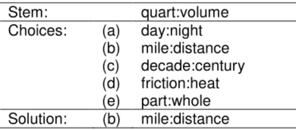
This sketch of LRA omits a few significant points. We will go through each step in more detail, using an example to illustrate the steps. Table 2 gives an example of a SAT question (Claman, 2000). Let’s suppose that we wish to calculate the relational similarity between the pair quart:volume and the pair mile:distance.
Table 2. A sample SAT question. Stem: quart:volume (a) day:night (b) mile:distance (c) decade:century (d) friction:heat Choices: (e) part:whole Solution: (b) mile:distance
1. Find alternates: Replace each word in each input pair with similar words. Look in
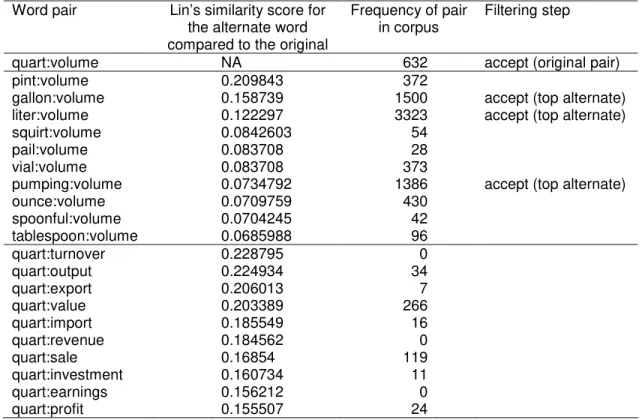
Lin’s (1998b) thesaurus for the top ten most similar words for each word in each pair. For a given word, Lin’s thesaurus has lists of similar words for each possible part of speech, but we assume that the part-of-speech of the given word is unknown. Lin’s thesaurus gives a numerical score for the attributional similarity of each word, compared to the given word, so we can merge the lists for each part of speech (when the given word has more than one possible part of speech) and sort the merged list by the numerical scores. When a word appears in two or more lists, only enter it once in the merged list, using its maximum score. For a given word pair, only substitute similar words for one member of the pair at a time (this constraint limits the divergence in meaning). Avoid similar words that seem unusual in any way (e.g., hyphenated words, words with three characters or less, words with non-alphabetical characters, multi-word phrases, and capitalized words). The first column in Table 3 shows the alternate pairs that are generated for the original pair quart:volume.
2. Filter alternates: Find how often each pair (originals and alternates) appears in the
corpus. Send a query to the WMTS to count the number of sequences of five consecutive words, such that one of the five words matches the first member of the pair and another of the five matches the second member of the pair (the order does not matter). For the pair quart:volume, the WMTS query is simply ‘[5]>(“quart”^”volume”)’. Sort the alternate pairs by their frequency. Take the top
three alternate pairs and reject the rest. Keep the original pair. The last column in Table 3 shows the pairs that are selected.
Table 3. Alternate forms of the original pair quart:volume. Word pair Lin’s similarity score for
the alternate word compared to the original
Frequency of pair in corpus
Filtering step
quart:volume NA 632 accept (original pair)
pint:volume 0.209843 372
gallon:volume 0.158739 1500 accept (top alternate) liter:volume 0.122297 3323 accept (top alternate)
squirt:volume 0.0842603 54
pail:volume 0.083708 28
vial:volume 0.083708 373
pumping:volume 0.0734792 1386 accept (top alternate)
ounce:volume 0.0709759 430 spoonful:volume 0.0704245 42 tablespoon:volume 0.0685988 96 quart:turnover 0.228795 0 quart:output 0.224934 34 quart:export 0.206013 7 quart:value 0.203389 266 quart:import 0.185549 16 quart:revenue 0.184562 0 quart:sale 0.16854 119 quart:investment 0.160734 11 quart:earnings 0.156212 0 quart:profit 0.155507 24
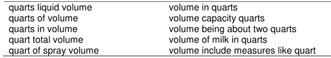
3. Find phrases: For each pair (originals and alternates), make a list of phrases in the
corpus that contain the pair. Query the WMTS for all phrases that begin with one member of the pair, end with the other member of the pair, and have one to three intervening words (i.e., a total of three to five words). We wish to ignore suffixes, so that a phrase such as “volume measured in quarts” will count as a match for quart:volume. The WMTS query syntax has an asterisk operator that matches suffixes (e.g., “quart*” will match both “quart” and “quarts”), but this operator is computationally intensive. Instead of using the asterisk operator, we use a few simple heuristics to add (or subtract) some of the most common suffixes to (or from) each word (e.g., “s”, “ing”, “ed”). For each pair, several queries are sent to the WMTS, specifying different suffixes (e.g., “quart” and “quarts”), different orders (e.g., phrases that start with “quart” and end with “volume”, and vice versa), and different numbers of intervening words (1, 2, or 3). Note that a nonsensical suffix does no harm; the query simply returns no matching phrases. This step is relatively easy with the WMTS, since it is designed for passage retrieval. With a document retrieval search engine, it would be necessary to fetch each document that matches a query, and then scan through the document, looking for the phrase that matches the query. The WMTS simply returns a list of the phrases that match the query. Table 4 gives some examples of phrases in the corpus that match the pair quart:volume.
Table 4 Phrases that contain quart:volume. quarts liquid volume volume in quarts quarts of volume volume capacity quarts quarts in volume volume being about two quarts quart total volume volume of milk in quarts
quart of spray volume volume include measures like quart
4. Find patterns: For each phrase that is found in the previous step, build patterns
from the intervening words. A pattern is constructed by replacing any or all or none of the intervening words with a wild card. For example, the phrase “quart of spray volume” contains the intervening sequence “of spray”, which yields four patterns, “of spray”, “* spray”, “of *”, and “* *”, where “*” is the wild card. This step can produce millions of patterns, given a couple of thousand input pairs. Keep the top 4,000 most frequent patterns and throw away the rest. To count the frequencies of the patterns, scan through the lists of phrases sequentially, generate patterns from each phrase,
and put the patterns in a database.8 The patterns are key fields in the database and
the frequencies are the corresponding value fields. The first time a pattern is encountered, its frequency is set to one. The frequency is incremented each time the pattern is encountered with a new pair. After all of the phrases have been processed, the top 4,000 patterns can easily be extracted from the database.
5. Map pairs to rows: In preparation for building the matrix X, create a mapping of word pairs to row numbers. Assign a row number to each word pair (originals and alternates), unless a word pair has no corresponding phrases (from step 3). If a word pair has no phrases, the corresponding row vector would be a zero vector, so there is no point to including it in the matrix. For each word pair A:B, create a row for A:B and another row for B:A. This will make the matrix more symmetrical, reflecting our knowledge that the relational similarity between A:B and C:D should be the same as the relational similarity between B:A and D:C. The intent is to assist SVD by enforcing this symmetry in the matrix.
6. Map patterns to columns: Create a mapping of the top 4,000 patterns to column
numbers. Since the patterns have been selected for their high frequency, it is not likely that any of the column vectors will be zero vectors (unless the input set of pairs is small or the words are very rare). For each pattern, P, create a column for “word1 P word2” and another column for “word2 P word1”. For example, the frequency of “quarts of volume” will be distinguished from the frequency of “volume of quarts”. Thus there will be 8,000 columns.
7. Generate a sparse matrix: Generate the matrix X in sparse matrix format, suitable
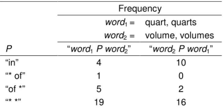
for input to SVDLIBC. The value for the cell in row i and column j is the frequency of the j-th pattern (see step 6) in phrases that contain the i-th word pair (see step 5). We do not issue queries to the WMTS to obtain these frequencies, since we found it faster to sequentially scan the lists of phrases from step 3, counting the number of pattern matches. Table 5 gives some examples of pattern frequencies for quart:volume. A pattern of N tokens (words or wild cards) can only match phrases in which there are exactly N intervening words (i.e., phrases in which there are a total of N+2 words; N = 1, 2, 3). A wild card can match any word, but one wild card can only match one word.
8
Table 5. Frequencies of various patterns for quart:volume Frequency
word1 = quart, quarts
word2 = volume, volumes
P “word1 P word2” “word2 P word1”
“in” 4 10
“* of” 1 0
“of *” 5 2
“* *” 19 16
8. Calculate entropy: Apply log and entropy transformations to the sparse matrix
(Landauer and Dumais, 1997). These transformations have been found to be very
helpful for information retrieval (Harman, 1986; Dumais, 1990). Let xi,j be the cell in
row i and column j of the matrix X from step 7. Let m be the number of rows in X
and let n be the number of columns. We wish to weight the cell xi,j by the entropy
of the j-th column. To calculate the entropy of the column, we need to convert the
column into a vector of probabilities. Let pi,j be the probability of xi,j, calculated by
normalizing the column vector so that the sum of the elements is one,
= = m k j k j i j i x x p 1 , ,
, . The entropy of the j-th column is then
= − = m k j k j k j p p H 1 , , log( ).
Entropy is at its maximum when pi,j is a uniform distribution, pi,j =1/m, in which
case Hj =log(m). Entropy is at its minimum when pi,j is 1 for some value of i and 0
for all other values of i, in which case Hj =0. We want to give more weight to
columns (patterns) with frequencies that vary substantially from one row (word pair) to the next, and less weight to columns that are uniform. Therefore we weight the cell
j i
x, by wj =1−Hj /log(m), which varies from 0 when pi,j is uniform to 1 when
entropy is minimal. We also apply the log transformation to frequencies, log(xi,j +1).
For all i and all j, replace the original value xi,j in X by the new value wj log(xi,j +1).
This is similar to the TF-IDF transformation (Term Frequency-Inverse Document Frequency) that is familiar in information retrieval (Salton and Buckley, 1988; Baeza-Yates and Ribeiro-Neto,1999).
9. Apply SVD: After the log and entropy transformations have been applied to the
matrix X, run SVDLIBC. This produces the matrices U, Σ, and V, where
T
V U
X= Σ . In the subsequent steps, we will be calculating cosines for row vectors.
For this purpose, we can simplify calculations by dropping V. The cosine of two
vectors is their dot product, after they have been normalized to unit length. The
matrix XXT
contains the dot products of all of the row vectors. We can find the dot product of the i-th and j-th row vectors by looking at the cell in row i, column j of the
matrix XXT . Since VTV=I, we have T T T T T T T T
) ( ) ( Σ = Σ Σ = Σ Σ Σ =U V U V U V V U U U XX ,
which means that we can calculate cosines with the smaller matrix UΣ, instead of
using T
V U
X= Σ (Deerwester et al., 1990).
10. Projection: Calculate UkΣk, where k =300. The matrix UkΣk has the same number
compare two word pairs by calculating the cosine of the corresponding row vectors in k
kΣ
U . The row vector for each word pair has been projected from the original 8,000
dimensional space into a new 300 dimensional space. The value k =300 is
recommended by Landauer and Dumais (1997) for measuring the attributional similarity between words. We investigate other values in Section 5.
11. Evaluate alternates: Let A:B and C:D be two word pairs in the input set. Assume
that we want to measure their relational similarity. From step 2, we have four versions of A:B, the original pair and three alternate pairs. Likewise, we have four versions of C:D. Therefore we have sixteen ways to compare a version of A:B with a
version of C:D. Look for the row vectors in UkΣk that correspond to the four versions
of A:B and the four versions of C:D and calculate the sixteen cosines. For example, suppose A:B is quart:volume and C:D is mile:distance. Table 6 gives the cosines for the sixteen combinations. A:B::C:D expresses the analogy “A is to B as C is to D”.
Table 6. The sixteen combinations and their cosines.
Word pairs Cosine Cosine original pairs
quart:volume::mile:distance 0.524568 yes (original pairs) quart:volume::feet:distance 0.463552 quart:volume::mile:length 0.634493 yes quart:volume::length:distance 0.498858 liter:volume::mile:distance 0.735634 yes liter:volume::feet:distance 0.686983 yes liter:volume::mile:length 0.744999 yes liter:volume::length:distance 0.576477 yes gallon:volume::mile:distance 0.763385 yes gallon:volume::feet:distance 0.709965 yes
gallon:volume::mile:length 0.781394 yes (highest cosine) gallon:volume::length:distance 0.614685 yes
pumping:volume::mile:distance 0.411644 pumping:volume::feet:distance 0.439250 pumping:volume::mile:length 0.446202 pumping:volume::length:distance 0.490511
12. Calculate relational similarity: The relational similarity between A:B and C:D is the
average of the cosines, among the sixteen cosines from step 11, that are greater than or equal to the cosine of the original pairs. For quart:volume and mile:distance, the third column in Table 6 shows which reformulations are used to calculate the average. For these two pairs, the average of the selected cosines is 0.677258. Table 7 gives the cosines for the sample SAT question, introduced in Table 2. The choice pair with the highest average cosine (column three in the table) is the solution for this question; LRA answers the question correctly. For comparison, column four gives the cosines for the original pairs and column five gives the highest cosine (the maximum over the sixteen reformulations). For this particular SAT question, there is one choice that has the highest cosine for all three columns (choice (b)), although this is not true in general. However, note that the gap between the first choice (b) and the second choice (d) is largest for the average cosines.
Table 7. Cosines for the sample SAT question.
Average Original Highest
Stem: quart:volume cosines cosines cosines
(a) day:night 0.373725 0.326610 0.443079 (b) mile:distance 0.677258 0.524568 0.781394 (c) decade:century 0.388504 0.327201 0.469610 (d) friction:heat 0.427860 0.336138 0.551676 Choices: (e) part:whole 0.370172 0.329997 0.408357 Solution: (b) mile:distance 0.677258 0.524568 0.781394 Gap: (b)-(d) 0.249398 0.188430 0.229718
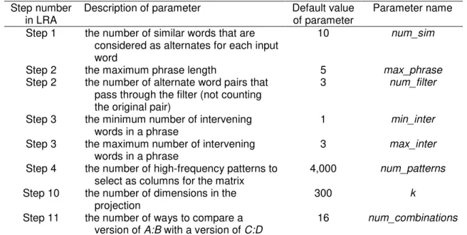
Steps 11 and 12 can be repeated for each two input pairs that are to be compared. Table 8 lists the numerical parameters in LRA and the step in which each parameter appears. The value of max_phrase is set to max_inter + 2 and the value of num_combinations is (num_filter + 1)2. The remaining parameters have been set to arbitrary values (see Section 7).
Table 8. Numerical parameters in LRA. Step number
in LRA
Description of parameter Default value of parameter
Parameter name Step 1 the number of similar words that are
considered as alternates for each input word
10 num_sim
Step 2 the maximum phrase length 5 max_phrase
Step 2 the number of alternate word pairs that pass through the filter (not counting the original pair)
3 num_filter
Step 3 the minimum number of intervening words in a phrase
1 min_inter
Step 3 the maximum number of intervening words in a phrase
3 max_inter
Step 4 the number of high-frequency patterns to select as columns for the matrix
4,000 num_patterns
Step 10 the number of dimensions in the projection
300 k
Step 11 the number of ways to compare a version of A:B with a version of C:D
16 num_combinations
5 Experiments with Word Analogy Questions
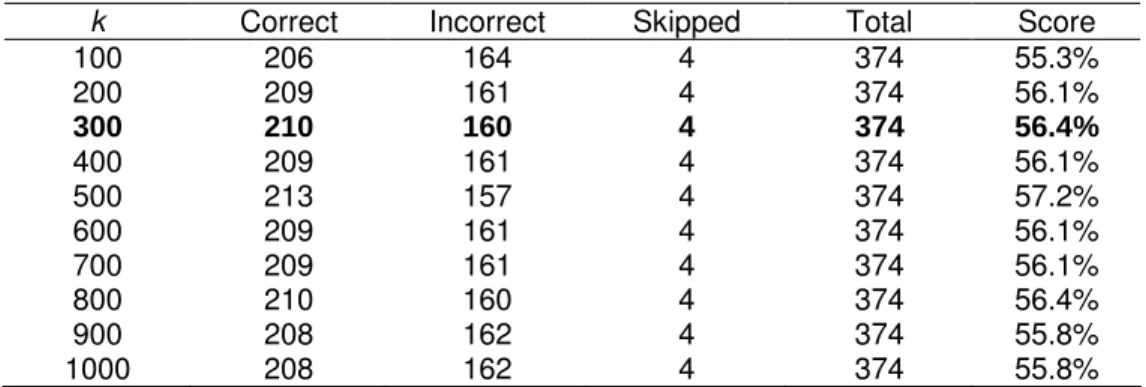
This section presents various experiments with 374 multiple-choice SAT word analogy questions (Turney and Littman, 2003b, 2005). Section 5.1 evaluates LRA, exactly as described in the previous section, with the 374 questions. Section 5.2 compares the performance of LRA to related work and Section 5.3 looks at human performance on the questions. Section 5.4 examines the effect of varying k, the number of dimensions for the SVD projection (step 10 in Section 4). The remaining subsections perform ablation experiments, exploring the consequences of removing some steps from LRA.
5.1 Baseline LRA System
LRA correctly answered 210 of the 374 questions. 160 questions were answered incorrectly and 4 questions were skipped, because the stem pair and its alternates were
represented by zero vectors. For example, one of the skipped questions had the stem heckler:disconcert (solution: heckler:disconcert::lobbyist:persuade). These two words did not appear together in the WMTS corpus, in any phrase of five words or less, so they were dropped in step 5 (Section 4), since they would be represented by a zero vector. Furthermore, none of the 20 alternate pairs (from step 1) appeared together in any phrase of five words or less.
Since there are five choices for each question, we would expect to answer 20% of the questions correctly by random guessing. Following Turney et al. (2003), we score the performance by giving one point for each correct answer and 0.2 points for each skipped question, so LRA attained a score of 56.4% on the 374 SAT questions.
With 374 questions and 6 word pairs per question (one stem and five choices), there are 2,244 pairs in the input set. In step 2, introducing alternate pairs multiplies the number of pairs by four, resulting in 8,976 pairs. In step 5, for each pair A:B, we add B:A, yielding 17,952 pairs. However, some pairs are dropped because they correspond to zero vectors (they do not appear together in a window of five words in the WMTS corpus). Also, a few words do not appear in Lin’s thesaurus, and some word pairs appear twice in the SAT questions (e.g., lion:cat). The sparse matrix (step 7) has 17,232 rows (word pairs) and 8,000 columns (patterns), with a density of 5.8% (percentage of nonzero values).
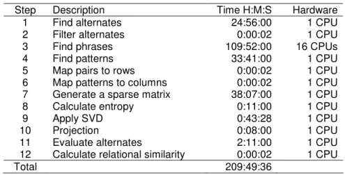
Table 9 gives the time required for each step of LRA, a total of almost nine days. All of the steps used a single CPU on a desktop computer, except step 3, finding the phrases for each word pair, which used a 16 CPU Beowulf cluster. Most of the other steps are parallelizable; with a bit of programming effort, they could also be executed on the Beowulf cluster. All CPUs (both desktop and cluster) were 2.4 GHz Intel Xeons. The desktop computer had 2 GB of RAM and the cluster had a total of 16 GB of RAM.
Table 9. LRA elapsed run time.
Step Description Time H:M:S Hardware
1 Find alternates 24:56:00 1 CPU
2 Filter alternates 0:00:02 1 CPU
3 Find phrases 109:52:00 16 CPUs
4 Find patterns 33:41:00 1 CPU
5 Map pairs to rows 0:00:02 1 CPU
6 Map patterns to columns 0:00:02 1 CPU 7 Generate a sparse matrix 38:07:00 1 CPU
8 Calculate entropy 0:11:00 1 CPU
9 Apply SVD 0:43:28 1 CPU
10 Projection 0:08:00 1 CPU
11 Evaluate alternates 2:11:00 1 CPU
12 Calculate relational similarity 0:00:02 1 CPU
Total 209:49:36
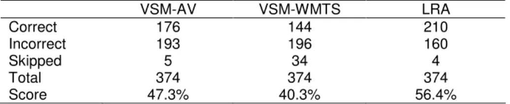
5.2 LRA versus VSM and PRMC
Table 10 compares LRA to the Vector Space Model with the 374 analogy questions. VSM-AV refers to the VSM using AltaVista’s database as a corpus. The VSM-AV results are taken from Turney and Littman (2003b, 2005). As mentioned in Section 3, we
estimate this corpus contained about 5 x 10¹¹ English words at the time the VSM-AV
experiments took place. Turney and Littman (2003b, 2005) gave an estimate of 1 x 10¹¹
refers to the VSM using the WMTS, which contains about 5 x 10¹⁰ English words.9 We generated the VSM-WMTS results by adapting the VSM to the WMTS. The algorithm is slightly different from Turney and Littman (2003b, 2005), because we used passage frequencies instead of document frequencies.
Table 10. LRA versus VSM with 374 SAT analogy questions.
VSM-AV VSM-WMTS LRA Correct 176 144 210 Incorrect 193 196 160 Skipped 5 34 4 Total 374 374 374 Score 47.3% 40.3% 56.4%
All three pairwise differences in the three scores in Table 10 are statistically significant with 95% confidence, using the Fisher Exact Test. Using the same corpus as the VSM, LRA achieves a score of 56% whereas the VSM achieves a score of 40%, an absolute difference of 16% and a relative improvement of 40%. When VSM has a corpus ten times larger than LRA’s corpus, LRA is still ahead, with an absolute difference of 9% and a relative improvement of 19%.
Comparing VSM-AV to VSM-WMTS, the smaller corpus has reduced the score of the VSM, but much of the drop is due to the larger number of questions that were skipped (34 for VSM-WMTS versus 5 for VSM-AV). With the smaller corpus, many more of the input word pairs simply do not appear together in short phrases in the corpus. LRA is able to answer as many questions as VSM-AV, although it uses the same corpus as VSM-WMTS, because Lin’s thesaurus allows LRA to substitute synonyms for words that are not in the corpus.
VSM-AV required 17 days to process the 374 analogy questions (Turney and Littman, 2003b, 2005), compared to 9 days for LRA. As a courtesy to AltaVista, Turney and Littman (2003b, 2005) inserted a five second delay between each query. Since the WMTS is running locally, there is no need for delays. VSM-WMTS processed the questions in only one day.
Table 11 compares LRA to Product Rule Module Combination (Turney et al., 2003). The results for PRMC are taken from Turney et al. (2003). Since PRMC is a supervised algorithm, 274 of the analogy questions are used for training and 100 are used for testing. Results are given for two different splits of the questions.
Table 11. LRA versus PRMC with 100 SAT questions. Testing subset #1 Testing subset #2
PRMC LRA PRMC LRA Correct 45 51 55 59 Incorrect 55 49 45 39 Skipped 0 0 0 2 Total 100 100 100 100 Score 45.0% 51.0% 55.0% 59.4%
Due to the relatively small sample size (100 questions instead of 374), the differences between LRA and PRMC are not statistically significant with 95% confidence. However,
9