A branching fuzzy-logic classifier for building optimization

A Branching Fuzzy-Logic Classifier for Building Optimization

Massachusetts Institute of Technology, 2003

SUBMITTED TO THE DEPARTMENT OF MECHANICAL ENGINEERING IN PARTIAL FULFILLMENT OF THE REQUIREMENTS FOR THE DEGREE OF

DOCTOR OF PHILOSOPHY IN MECHANICAL ENGINEERING AT THE

MASSACHUSETTS INSTITUTE OF TECHNOLOGY

JUNE 2005

MASSACHUSETTS INST1

OF TECHNOLOGY

© 2005 Matthew Lehar. All rights reserved.

JUN

2

2005

'I

/LIBRARIES

Signature of Author:

Certified by:

Accepted by:

e(

Department of Mechanical Engineering

- // May 26,2005

Leon R. Glicksman Professor of Architecture and Mechanical Engineering Thesis Supervisor

A Branching Fuzzy-Logic Classifier for Building Optimization

By

Matthew A. Lehar

Submitted to the Department of Mechanical Engineering on May 19, 2005 in Partial Fulfillment of the Requirements for the Degree of Doctor of Philosophy in

Mechanical Engineering

ABSTRACT

We present an input-output model that learns to emulate a complex building simulation of high dimensionality. Many multi-dimensional systems are dominated by the behavior of a small number of inputs over a limited range of input variation. Some also exhibit a tendency to respond relatively strongly to certain inputs over small ranges, and to other

inputs over very large ranges of input variation. A branching linear discriminant can be used to isolate regions of local linearity in the input space, while also capturing the effects of scale. The quality of the classification may be improved by using a fuzzy preference relation to classify input configurations that are not well handled by the linear discriminant.

Thesis Supervisor: Leon Glicksman

Acknowledgments

I would like to thank the Permasteelisa Group for their sponsorship of the MIT Design Advisor generally, and my graduate studies in particular. I am also extremely grateful for the generous support of the Cambridge-MIT Institute and the Martin Family Society of Graduate Fellowships in Sustainability.

Jim Gouldstone's programming expertise has played an important role in the success of this project. The web interface would not have been possible without his guidance.

I am grateful to Les Norford and Dave Wallace for agreeing to join my thesis committee and for their help and suggestions.

Thank-you so much, Leon, for providing the inspiration for this project and for all your help in making it happen. The weekly meetings were very valuable to me.

Lots of love to Mum and Dad.

TABLE OF CONTENTS

INTRODUCTION 6

Background: The MIT Design Advisor 6

Strategies for Pattern Recognition 8

LINEAR METHODS: EMULATING THE BEHAVIOR OF PHYSICAL MODELS 14

Introduction ₁₄

Linear Regression ₁₆

Method of Subdivisions 21

Binary Classification 25

The Fisher Discriminant ₂₈

THE MEMBRANE ALGORITHM: REFINEMENTS BASED ON STATISTICAL

TOOLS 38

Introduction 38

Membrane Model 40

Weighting Information from Multiple Histograms 48

Discussion of the Weighting Criteria 51

Measuring the Aberration 55

Reconciling the Experts 57

The Fuzzy Preference Relation ₅₈

Fuzzy Decision Making ₆₇

Configuring the Membrane ₆₉

REAL-TIME OPTIMIZATION WITH SIMULATED ANNEALING 72

Overview of the Simulated Annealing Procedure 72 STRUCTURE OF THE COMPUTER PROGRAM 83

Functional Modules and Their Responsibilities 83

DESIGN OF A USER INTERFACE 90

Graphical Layout of the User Interface 90

User Control of Optimization ₉₁

Error Checking Procedure ₉₂

Further Accuracy Improvements 93

RESULTS 1: ACCURACY OF THE ESTIMATOR 96

Accuracy Criterion ₉₆

Performance Statistics ₉₆

Validation of Coding Strategies 100

RESULTS 2: OPTIMAL TUNING OF THE ANNEALING ALGORITHM 102 RESULTS 3: SENSITIVITY ANALYSIS FOR OPTIMAL BUILDINGS 105

INTRODUCTION

Background: The MIT Design Advisor

The web-based design tool known as the "MIT Design Advisor"[1] has been in

development in the Building Technology Lab since 1999. Online and freely available to

the Internet community since 2001, the tool has been substantially expanded from its

original role as a heat-transfer model for building facades. Presently, users can access

daylighting and comfort visualizations, check their buildings against various code

restrictions, simulate both mechanical and natural modes of ventilation, and receive total

cost estimates for energy consumption over the building lifetime.

The tool is designed to be used in the early stages of a building project, at a point when

architects are still entertaining a range of different ideas about siting, general plan outline,

window coverage, and other basic design issues. Accordingly, the design specifications

that the user is asked to enter (Fig. 1), and which are then used in simulation programs to

produce estimates of monthly energy usage by the building, are general in nature

(although users wishing to use more detailed constraints can open submenus where they

may be entered).

C 250 N 250 250 C 500

.Yearly

200 200 _200 400 Monthly

150 150 150 300 Heating energy required per square meter of plan.

100 100 100 200 BLUE

4 ... ... ... .. . .... -Cooling energy required per square meter of plan.

50 50 50 100 GREEN

. .. Lighting energy required

-- --- - per square meter of plan.

(Kilowatt-hours / meter2)

Fig. 2. View of the Design Advisor website showing energy consumptions calculated for 3 buildings.

The benefit of using a tool like the Design Advisor derives from the ability to compare

many different configurations of building on the basis of the amount of energy consumed.

The present version of the software includes the facility to save four different

configurations at once, so that their heating, cooling and electrical lighting consumption

parameters are varied, it has still been difficult for users to discover how the more than 40

different inputs defining the building can be conjointly varied in such a way as to bring

energy savings. This would require an automatic feature for optimizing multiple

parameters simultaneously in the building model. This thesis presents a possible

algorithm for such an optimization tool. Finding a robust methodology for incrementally

choosing and testing increasingly efficient combinations of input parameters is a problem

that has substantially been solved in other arenas. The principal part of the work

presented here concerns the problem of developing an allegory-function to substitute for

the physical building simulations used by the Design Advisor. Those models, which

have been verified at an accuracy of more than 85% by third-party tools, rely on physical descriptions of the conductive, convective, and radiative behavior of building facades and

interior cavities. Although they rely on substantial simplifications of the building model,

they still require about 5 seconds of processing time to produce energy estimates for each

new building configuration, which is impractical for a large-scale optimization

incorporating hundreds of thousands of trials. Instead of running these models directly in

the optimization process, we have constructed a non-physical input-output model that can

be trained to reproduce the behavior of the physical models approximately, and that runs

in a tiny fraction of the time.

Strategies for Pattern Recognition

At the heart of the problem of creating an input-output model is the task of pattern

recognition. Given a set of sample input values and the outputs they produce, the model

regression, in which a general form is assumed for the function and its coefficients are

adjusted so that expression predicts the sample output values with minimum error. To match the function to the sample data so that it will correctly predict any new output, the equation should be of the same order as the data. Pattern recognition techniques

traditionally treat the modeled phenomena as though they can be classified as

fundamentally linear, quadratic, cubic, or of some higher order. If a low-order model is used to estimate data in a high-order problem, the presumed function will not estimate the sample outputs with great accuracy (Fig. 3a). If, on the other hand, the problem is of low-order and a high-order model has been applied to it, the result is a function that can be tuned to reproduce the sample outputs exactly, but that also imposes convolutions unsupported by the data that prevent the correct estimation of future output values (Fig.

* Sample point

OUTPUT ... True function

-- Polynomial estimate ** INPUT a. OUTPUT INPUT b.

Fig. 3. Estimating a function using sample points. In a.), the estimation is of a low order, and the curve does not model the sample points with much accuracy. In b.), the order is increased and all sample points are exactly intersected, yet the estimation produces artifacts not present in the original function.

The effectiveness of polynomial-fitting procedures, along with other basis-function techniques such as neural networks, is limited by the difficulty of extracting general rules

from the training data. To be able to assign the correct output to each fresh input value encountered after the completion of the training process, the algorithm must have some way of deciding to what extent the sample data represents the larger reality of the phenomenon that created it. The special information that each point provides is to some

extent merely the result of its accidental selection for the training set from among many possible neighboring points in the input space.

The GMDH (Group Method of Data Handling) approach of Ivakhnenko[2] uses an estimation routine that attempts to resolve this problem by adaptively matching the order of the model to that of the underlying phenomenon represented by the training data, and work has been carried out (see Farlow[3]) to expand the technique to a larger class of non-polynomial basis functions as well. But in addition to the problem of order-matching, the basic assumption that the phenomenon to be modeled has the form of a combination of basis functions may itself be problematic. Since any function can be arbitrarily well approximated by a Taylor series (or Fourier series, etc.) about a particular point, the presumption of this underlying polynomial behavior can be shown to be valid locally, but it may not capture the complete variation in a problem over a range of input values.

A simple approach we have used to avoid this difficulty in our building performance

application is to organize training data into histograms (see the chapter on The Membrane

input axis. The output values in the lookup table are averages taken over all sample data that fall within a particular interval of input values (Fig. 4). Such a table can reproduce with arbitrary accuracy the function underlying the sample data (Fig. 5), provided that a large enough supply of data is used and the "bins" into which neighboring data are grouped cover a suitably narrow range of input values.

80-....---- '-" 40 . -. - -4 . _4.. 1-: INPUT: OUTPUT: 0L 70-80 62.3 60-70 49.5 50-60 32.8 40-50 59.6 30-40 74.9 20-30 51.3 10-20 15.9 0-10 22.7

Fig. 4. Construction of a lookup table. EL

0

OUTPUT

INPUT

Fig. 5. Representation of a function in one dimension using a histogram.

The obvious disadvantage of this method over basis-function methods is the difficulty of extending it to a problem with multiple input dimensions. The accuracy of the histogram representation of a function depends on the density of points along a given input axis. In our single-input example, a sample size of 100 points would provide a maximum

resolution of 100 pixels with which to render of the output-generating function using the lookup table. In the case of a function in two inputs, the same sample size would characterize the 3-dimensional plot of the function surface with a resolution of only

(100)1/2 = 10 pixels in each dimension. As we will explain in the chapter, The Membrane

Algorithm, the problem of representing data in multiple dimensions with histograms can

be solved by using a series of 1-dimensional histograms, rather than a single, multi-dimensional one.

LINEAR METHODS: EMULATING THE BEHAVIOR OF PHYSICAL

MODELS

Introduction

The problem of optimizing our existing physical building model is straightforward. We

select an optimization algorithm appropriate to the large number of varying inputs, such

as Simulated Annealing, and the output from each run of the model provides an objective

function for the Annealing algorithm. Each run of the model takes approximately 10

seconds and, since many thousands of cycles are required for the Annealing algorithm to

stabilize, an entire optimization should take several hours. Unfortunately, this is too long

to wait in the context of our particular application.

The principal use of the optimizer will be as a feature of the Design Advisor, allowing

users to find a lowest-energy building configuration. The user will be able to fix any

number of input values as exogenous to the optimization problem, so each optimized

building configuration will be unique to the particular choices made by each user.

Consequently, each new optimization must be performed in real-time as the user requests

it. Since running an optimization by using our original building simulation to calculate

values of the objective function would take hours, this cannot be the basis of a real-time

optimizer. Instead, we must develop a substitute for the original model to run in a

To create an emulator of the physical building model, we propose a rule-learning

algorithm that can be trained using results generated by the physical model to imitate the model's behavior. We will refer to the total annual energy requirement that the physical model calculates for the building as the output. The physical model transforms a set of input values - the input vector - into a single value of the objective function - the sum of the heating, cooling, and lighting energy that a building defined by those input

parameters will require for one year of operation. In our application (buildings),

properties such as window reflectivity or room depth are the input parameters that make up an input vector. When enough input vectors have been evaluated by the physical model, we can begin to make crude approximations of the values of the objective function that correspond to new and untried input vectors. The role of the emulator is to estimate the objective function for any input vector by finding rules that link the already-evaluated input vectors with the values of the objective function they have been found to correspond to. The emulator uses only the results produced by the physical model to construct its rules, without reference to the equations of heat transfer used in the original model. It should be able to operate many orders of magnitude faster than a detailed physical simulation.

In the interest of speed, we would like to use the simplest possible algorithm to

approximate the behavior of the building model. A lookup table could be used if not for the large number of input variables involved in the simulation. Presently, over 40 are used in the Design Advisor interface, implying a 40-dimensional input space. To

a trend along any given axis of movement within the space would require 24, or about a

trillion, training data. Using a Pentium III processor at 1 GHz, it would take 322,000

years to accumulate so many results by running the original model, not to speak of the

problem of storing and accessing such a library. Clearly, such a scheme would be

impractical due to the large number of input parameters.

Linear Regression

One naive scheme for estimating the output value that results from a large suite of inputs

is to use a linear regression. The input values are each multiplied by some constant

coefficient that best captures the sensitivity of the output to that variable, and the scaled

input values are then added together to make a predicted output value:

Output = a,X, +a2X 2 +a3X3.a aX, (a1n)

In set-theoretic terms, the role of a linear regression is to provide an ordering rule for a

set of training data. If the linear prediction of an output value is given by the dot product

W -X = Output , where W is a vector of weighting coefficients, then W is a unique way to

order the training data input vectors X such that their predicted outputs are monotonically

increasing. For a set of n data,

W -X 1 >W - X,Vi < n (2)

To imitate the dynamics in the building model effectively, we must use a scheme that can

accommodate nonlinearity in the training data. Because nonlinear functions are not

The values of the objective function Fi from a nonlinear training set provide a measure of the inaccuracy of the regression in the magnitude of a set D, where

D={X,W e RL :W .X >W -XiF(Xj)< F(Xi),Vi < j 5 n (3)

This set of points D, which we call the set of misordered points, is shown graphically in

Fig. 6 for a two-dimensional input space. The nonlinearity of the function in Fig. 6 is

Input 2 * Output > median x Output <median N N i~~NN N N N ~ 4~ N. N N ~ N N W-Vector 0 Input 1 11X IAN egion of Overlap Span of input values projected along the vector W

Class 1 Domain (lower output) Min. Projection CIs Dmi Class 2 Domain (highe r output) Re oin of Overmp

Fig. 6. A function of two inputs. The vector W is oriented in the 2-dimensional input space so as to order the data in accordance with the output values. In the Region of Overlap the data are out of order in respect to their output values, defining a set D.

The particular vector W used in the regression can be said to be optimal on a set

{X

I|DJJ

represented by any linear regression, the set of training data that follows a nonlinear

objective function will have an associated minimum set D that is nonempty. We can

measure the degree to which a subset of the training data submits to a linear ordering

using the average predictive accuracy , the ratio of monotonically ordered points n

to the total number of training points n that are used in the regression. This measure of

the accuracy of a regression will depend on two factors:

1) _{The particular coordinates in the input space where the regression is centered,} and

2) The subset of n training data used to determine D in the vicinity of those

coordinates.

Regression

I Line

INPUT

Regression

Subset

The regression approximates F over the range of input vectors included in a subset of the

training data. The slope of the regression line in Fig. 7 represents the vector of

coefficients W, and is chosen so as to minimize the deviation of the line from a limited

set of neighboring data points. If we assume the objective function F is continuous, for a

given vector of weighting coefficients Wo we can show that the accuracy of prediction

I I approaches 1 in the limit as we reduce the interval defining the region of the

n

input space from which training data may be used in the regression:

First, we define a set B representing any monotonic interval in a continuous nonlinear

function: if

" S is the initial set of training data X e R L : X1,X2,...Xn,

* D is the set of misordered points resulting from the ordering of S by WO, and

" the set S - D is nonempty,

there exists a subset of vectors Br c S containing a vector X such that:

B, r= {X : W -_X > W -X, -:> F(Xj) F(X),VX C S :I(X - Xo)I< r (4)

where r is a scalar. Such a subset is illustrated for the single-input case in Fig. 7, over

which the behavior of the function is monotonic. For a single Xo within S, we can define

aF

a distance p between the vector Xo and the nearest point for which W = 0 , where X"

aXa is any scalar component of X. Then, for any Xo defined on F,

This is to say that the function F is monotonic within a range p of Xo. From ( 4 ), we see that within a training set S there always exists some set of coordinates B for which the outputs vary monotonically with the ordering provided by Wo. ( 5 ) allows us to

determine the bounds on the largest monotonic set BP that contains X; since a continuous function is by definition monotonic between points where partial derivatives of the function equal 0, we will end up with a monotonic set simply by narrowing the radius of inclusion r until r < p . This means that the accuracy of a linear regression will generally improve as data more remote from a chosen reference point X are removed from the regression calculation. However, although we are able to evaluate a given input more and more accurately in the context of the other points that remain in the regression, we lose the ability to evaluate it relative to the entire training set. The quality of the local ordering of points in the subset improves while the global ordering disappears. There is no "ideal" regression to characterize a particular region of the input space because narrowing the scope of input points in the regression to increase the linearity also makes the regression less comprehensive.

Method of Subdivisions

For any given point in the input space, and given the ability to determine the weighting

vector W that minimizes - for a prescribed set of training data in the neighborhood

n

of the regression, we propose a method of multiple regressions that systematically divides

up the input space. This method is unconventional in the sense that the space is

repeatedly divided in half to create a branching hierarchy of divisions. Most other

methods (e.g. Savicky[4] and Hamamura[5]), rather than a segmenting, rather than

branching, approach is usually taken when using binary classifiers to represent multiple

output categories.

We begin by performing a regression on the entire training set. This will identify

linearity at the largest possible scale, but rather than finding an approximation to the

function using this very coarse regression, we would like instead to use it to put limits on

the range of possible output values. A second regression based on only those training

data that lie within the indicated range could then be performed, limiting the range still

further. After many such subdivisions of the space we would arrive at the point where

further regressions could not be justified due to the small number of chaotic distribution

of the remaining samples. At each decision point, where a set of training data is divided

into two distinct groups according to output, we create a linear regression that is special

to that decision point. What results is a "tree" of linear regressions calculated on the

basis of various subsets of the training data. This tree can then be used to classify new

input points by passing the component values down the tree to regressions that deal with

ever more specific regions of the input space. The reason for using this multi-stage

approach is that it exploits linearities in the data at a range of different scales, rather than

just at a small scale where a single regression is not comprehensive, or just at a large one

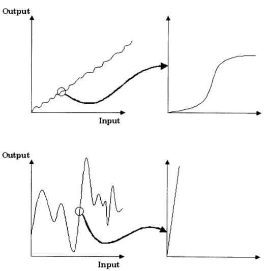
probable range of outputs that a new input point could evaluate to by noting the limits on the outputs of training data that were given the same classification - the same "slot" at the bottom of the tree.

Output

Output

Input

k

Input

Fig. 8. A broadly linear function (top) can display extreme nonlinearities at a finer scale. Conversely, a highly nonlinear function (bottom) can approximate linear behavior when taken over a small range.

Changes in the value of the function in respect to an input variable can resemble a linear

ab

reverse can also be true (see Fig. 8). Using a scheme of successive subdivisions of the

input space, we should be able to capture these linearities at many different scales.

The particular coordinates on which a regression should be centered at each stage of this

process are not known a priori. However, the multi-stage approach provides a way

around this problem: while it does not construct a regression for every possible grouping

of training data points it effectively subdivides the input space into successively smaller

contiguous data sets. Any single input vector will belong in one of these (arbitrarily

small) subsets, so that no matter which input we choose from the training data, it will be

associated with some regression constructed from its immediate neighbors. This

guarantees that the regression will be locally accurate. At the same time, we can learn

which of these local regressions we should use to evaluate an input by consulting the

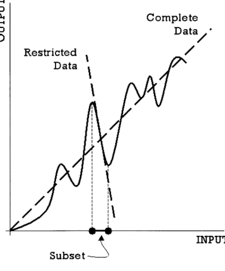
more general regressions in the next layer up in the branching structure. In Fig. 9, two

regression lines have been drawn: one follows the general trend of the function taking in

the full range of inputs. The other is based on a highly restricted range of inputs, and

only functions to distinguish output values within that narrow range. Using only the

restricted regression as an ordering for the entire data set would clearly be disastrous, but

it provides great accuracy if the crude regression is first used to identify the neighborhood

of values where the restricted one will be effective. From ( 5 ), we see that we eventually

arrive at a perfect linear ordering of a subset of data simply by narrowing the range of

that subset. This means that there will always be an accuracy benefit from narrowing the

successively narrower regressions, we can design a predictive algorithm that is both comprehensive and minutely accurate.

Complete

Data*

Restricted

Data

INPUT

Subset

Fig. 9. Two regression lines: one is based on the complete data set and the other on a restricted monotonic subset.

two. At the first branching point, the skier makes a very general choice, such as whether

to ski on the shaded or the sunlit side of the hill. As she proceeds to commit to one trail

or another at each fork, the quality of the decisions becomes more specific: a decision as

to which chairlift area she would prefer to end up in, and then whether to take the smooth

run or the one with moguls. Finally, she decides which of two available queues to turn

into for the chairlift ride back up the mountain. Her ultimate choice of a queue makes a

very specific distinction, but it can only be arrived at by a history of decisions at a more

general scale.

Like the skier who chooses a more and more specific route as she progresses down the

mountain, our multi-stage procedure uses a series of linear regressions to make

increasingly specific predictions of the value of an objective function. At each level of

the decision process, we preserve as much generality as possible, so as not to interfere

with the better resolving power of subsequent steps. We ensure this outcome by using

the regression functions to impose the weakest possible restriction at each level. The

vector w serves as a two-group classifier, projecting input vectors onto a scalar value that

is less than 0 if the input is selected for one group, and greater than 0 if it is selected for

class A

class B

+-

-

--

+

Fig. 10

The two-group (binary) classification tree is the most conservative possible scheme for

sorting input vectors because no distinction is made at any level of the tree that would

also be possible at the next level down. A decision about which general group a vector

belongs in does not bias or influence the next decision about which part of the selected

group should be chosen. The only new information added at each selection stage is an

identification of the next-most-specific subgroup to which an input will be assigned. We

could of course obey this same principle while choosing from among 3,5, or 100

subgroups at each level, but a 2-group scheme should in general be preferred because it

allows the subgroups to remain larger and the classifications less restrictive down to a

2-Class, 4 Levels

4-Class, 2 Levels

Fig. 11

The more layers of decision opportunities we have, the more individual regressions we

bring to bear on the classification and the more informed the ultimate prediction will be.

The Fisher Discriminant

The Fisher Discriminant is a regression technique that is often used as a criterion for

separating a group of samples into two categories based on their known parameters. If

some of the samples are arbitrarily designated as "Type A," and the others as "Type B," a

linear model can be built up to correlate the parameters of each sample optimally with its

specified type. For instance, if we were to classify cars on the highway as either "fast" or

"slow," we would do so according to whether their speed is above or below a chosen

threshold value. Then, the values of input parameters like engine size, body type, color,

and weight could be correlated with the side of the threshold on which the car is found.

Once the correlation has been established using this training data, it can be used to predict

whether a new car, whose type has not been observed, will likely be fast or slow based

In our experiment, the cars on the highway are replaced by the training data. These consist of a set of vectors (of parameters like size, color, and weight) for which values of the objective function (e.g. speed) are known in advance. Taking any subset of this data, we can choose an objective function value as a marker value that divides the subset into two parts: one containing the inputs for which the objective is below the marker value, and the other for which the objective exceeds the marker value. To divide a set of training vectors evenly in half, we would choose the median of the objective function values as the marker. If we create a linear regression from the training data, finding the linear combination of the components of each input vector that best approximates the objective function, we can use that regression to predict an objective value for any new input vector, and place it in one group or the other depending as the objective value is above or below the threshold.

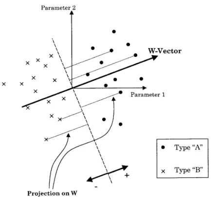
The Fisher Discriminant is a particular kind of regression that is optimized for the case in which we would like to separate data into two groups. Like any other regression, it projects the multi-dimensional parameter space onto a 1 -D vector traversing that space.

But instead of adjusting that vector (hereafter called w) so as to minimize the sum of the squares of the differences between each vector's true objective value and its predicted value, the Fisher Discriminant orients w so as to discriminate optimally between the two classes. The length of the projection of each measurement along w can then be used to classify it as either of group "A" or "B" (Fig. 12).

Parameter 2 x 0 0 \ W-Vector x x x X Parameter 1 X \ X ₀ * Type "A" x Type "B" Projection on W

Fig. 12. A line clearly divides the data into two classes in this example, in which the overall mean has been normalized to the origin of the coordinate system. Positive projections on W can be classified as "A," negative as "B."

There are many possible ways to "optimize" the orientation of w to discriminate between

two classes of data. The Fisher Discriminant uses two principal measures: the projection

of the mean difference vector on w, and the projection onto w of the spread of the data in

each of the two classes. The mean difference vector (a between-class metric) is the axis

along which the two groups of data are most distinct from each other; the spread of the

data (a within-class metric) shows how the positions of data points in each of the two

groups become more concentrated or more diffuse when measured along a given axis.

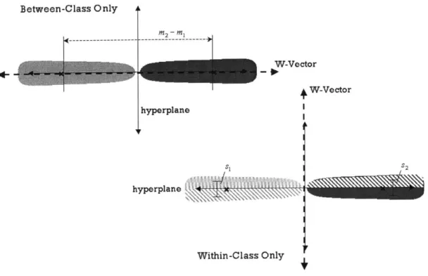
Optimizing one of these measurements to the exclusion of the other can result in a poor

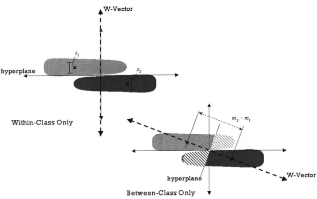
classification in certain circumstances. As shown in Fig. 13 and Fig. 14, either metric

Discriminant finds a compromise between the separation critera by optimizing both simultaneously. Between-Class Only -4--2 _ ₁ hyperplane hyperplane W-Vector W-Vector S 2 Within-Class Only

Fig. 13. Insufficiency of the within-class criterion alone. The input vectors are 2-dimensional, and the the regions of points representing groups A and B are shown in two shades of gray. The orientation of W (dashed line) that produces an optimal between-class separation is horizontal, allowing the data to be cleanly divided according to its projections on W. If the within-class criterion alone is used, W is vertical when the projections of the spread of data onto Win each group are minimized, yet these projections are insufficient to distinguish between the groups.

i~-, ~ - - -

-W-Vector

hyperplane 2

Within-Class Only IM2y

hyperplane W-Vector

Between-Class Only

Fig. 14. Insufficiency of the between-class criterion alone. In this example, the within-class spread provides the essential information for separating the two groups of data.

Between-Class Separation

The mean difference vector is oriented along the line connecting the point at the mean

coordinate values of the training inputs in one group (or class), and the mean point of

those in the other group. In Fig. 13 and Fig. 14 this vector is shown for the

two-parameter case. In the analysis that follows, m represents the vector (of 2 or more

dimensions) of mean values for each of the input parameters, taken over the set of data

points in group A or B. We wish to orient w parallel to the mean difference vector so that

the projection of the data points onto w shows the greatest possible separation between

the groups. We express the degree of alignment of the vector w with the mean difference

vector (mB -MA) as the dot product. Since the quantity w - (mB - MA) will be

SB = (MB mA_ mB M )T such that the scalar expression WTSBw , equivalent to the square of w .(mB -MA), is also maximized when w 1 (mB - M,). The parallel

alignment of w and (mB - mA) maximizes the projected distance between the clusters of each class of data.

Within-Class Separation

The other expression optimized in the Fisher Discriminant preferentially indicates orientations of w that emphasize the density of clustering within each class, as viewed through the projection onto w. Maximizing the clustering density reduces ambiguity due to two class regions overlapping in the input space. The clustering density is inversely related to the quantity WTS W , the within-class covariance matrix. SW is defined:

S, = M x"6-) + (x" -MBX T6) _(x

neCA neCB

where x is a vector representing a sample input. The diagonals of S, are the variances of each of the input parameters within class "A," added to the variances from class "B." The off-diagonal elements of S, are the covariances - the tendency of one component of the input vector to stray from the mean at the same time that another component strays from its own mean. If the components of the sample input vectors are chosen

independently, the covariances should converge to 0.

w TS w J(w) = B

w Sww

which is maximized when the between-class covariance is maximized, and the

within-class covariance minimized. To do so, we differentiate ( 7 ) with respect to w and set

dJ(w)

-o

dw

d (f(x) _f'(x)g(x) -f(x)g'(x).

By the quotient rule for matrices, d g'x)) 2 _{(x) . Applying this}

dx g (x) g2(X

rule to ( 8 ), we have

dJ(w) d(w TSBw) w Tsw w d(wS WW)w Ts Bw= ₍₉₎

dw dw dw

By the rules of matrix differentiation, d(XTCX) = 2Cx , so ( 9 ) becomes

dx

(wTsBWw = (WTSWW Bw (10)

Because we are only interested in the direction of w, and not the magnitude, we may drop

the scalar factors WTS Bw and WTS w. As we noted before, SBw has the same

direction as (mA - mB ), so we may write ( 10 ) as a proportional relationship,

wexc S-I(mB-mA) (11)

which we use as a formula for w.

Simplification for a One-Dimensional Space

The Fisher criterion given by ( 7 ) can be expressed in a more intuitive form if we

consider the case of only one input parameter for the data under consideration. The mean

single parameter, (mB-mA), and the matrix SB becomes a scalar with the value (mB-mA)2 .

The matrix S, can be seen to reduce to the sum of the within-class covariances of the two classes, where the within-class covariance is defined as s = (y" - mk)2 . In this

neCk

expression, y" is the (1 -D) parameter value of a single datum n within the group Ck , and

mk is the mean input value for that group. Eq. ( 7 ) can now be re-written as w2_(mB mA)2 J(w) =W2(B M) ,or 2(S2 +S 2) A(mB mA 2= 2 (12) SA ± B

giving the measure of the separateness of the two groups A and B in an input space of one dimension. The measure increases as the mean parameter values of the two groups get farther apart, and as the variation within each of the two groups is reduced.

Minimizing the Nonlinearity

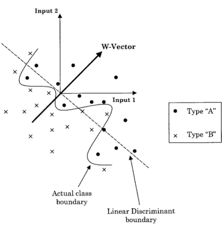
The purpose of this paper is to argue that the same methods used to classify data into two discrete categories are also effective at predicting functions with a continuous range of outputs. For continuous functions, the ability of any linear regression to characterize the output is limited by the nonlinearity of the function. In the case of a continuous linear function of many variables, the Fisher Discriminant can be used to exactly divide the input space into a region that will produce outputs below the mean value and a region producing outputs above the mean. In the case of a nonlinear function, the boundary

separate the data according to output values, but will be subject to a degree of

"interference" because the true division between output classes is not a straight line or flat plane (or hyperplane, in the case of 4 or more input dimensions), but a meandering boundary (Fig. 15). Input 2 L NNN W-Vector x NN NNN x NNN x x x \ x x Actual class boundary * Type "A" x Type "B" Linear Discriminant boundary

Fig. 15. The boundary between classes in a nonlinear function cannot be completely defined by a linear discriminant.

If our task were to separate the outputs from a nonlinear function into two classes,

above-and below-mean, with the minimum of interference, the Fisher Discriminant would provide a way to preferentially select those orientations of w that minimize the

mean separation to clustering density in the discrete two-class problem, would serve to indicate the level of interference between higher-than-mean output and lower-than-mean output in our hypothetical nonlinear function. A smaller value of J would indicate a more diffuse distribution of samples belonging to each class in the direction of w, and an increase in the region of overlap between the classes. J is equivalent to an inverse measure of nonlinearity in a given direction within the input space.

In our discussion of the method of subdivisions, we drew attention to the phenomenon of linearity at different scales (Fig. 8). The objective function we are trying to approximate can be fairly linear at one scale and extremely nonlinear at another. If we now vary one input parameter while keeping the others constant, we can observe that the objective function changes in a more linear way when we vary one input than it does when we vary another.

THE MEMBRANE ALGORITHM: REFINEMENTS BASED ON

STATISTICAL TOOLS

Introduction

However well the Fisher Discriminant succeeds in minimizing the region of overlap, we

are still left with the question of how well we can characterize a continuous function

simply by being able to place a sample input vector in the "above mean output" or

"below mean output" category. Even if the power of discrimination between these two

classes is great, we still have only determined the likely output of the function to a very

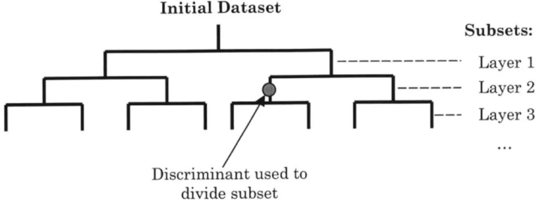
low resolution. To increase the resolution of the result, we use the discriminant

repeatedly, first dividing the entire data set along the mean output value and then

successively dividing up each resulting class along its class mean. Such an approach

gives a more resolved answer, but would not be expected to perform any better than a

straightforward linear regression, in which a final value of the function output is

Initial Dataset Subsets:

---

Fig. 16 By dividing the data set into successively smaller pairings, we approximate a continuous

representation of the output space

The Fisher algorithm orients w to minimize the diffuseness of each class, which has the effect of seeking linearity in the input space. To take full advantage of the special properties of the Fisher Discriminant, w must be recalculated at each level of the decomposition of the data set. A decomposition scheme in which w is successively recalculated has two main advantages over a simple regression formula:

" In general, a linear approximation will be more appropriate in respect to some

inputs than to others, but the emphasis on any given group of inputs, indicated

by an orientation of w that aligns more closely with them than with others,

will vary depending on the region of the input space in question. Different choices of W are appropriate for the different subsets of data being analyzed. * As we reach lower levels of the decomposition, the range of input values

under consideration becomes smaller. Changes in the value of the function in respect to an input variable can resemble a linear relationship over a large range, but become highly nonlinear at a smaller scale. The reverse can also be

true (see Linear Methods, Fig. 3). The optimal orientation for w can vary as

we home in on increasingly specific subsets of data.

Any orientation of the W-vector, no matter how carefully chosen, will necessarily

misclassify some inputs in a nonlinear problem. In our branching scheme, a

misclassification at the top of the decision tree is more serious than one that occurs lower

down. For example, the first classification is the most crude because it can only decide

whether a sample belongs in the upper or lower half of the entire catalogue of training

data. A misclassification at this level prevents the sample from participating in the

successively finer distinctions that occur at lower levels of the decision tree.

Membrane Model

As a way of correcting the misclassification of inputs at each level of the decision tree,

we have implemented a histogram method called a "Membrane." The Membrane

identifies mistakes made by the existing hierarchy of linear discriminants in classifying

the training data, and creates permanent structures that will adjust the classifications of

new inputs once the tree is completely "trained," and has been put into service as an

estimator. The idea of applying a correction to the classification provided by a linear

discriminant is not new; a method known as a Support Vector Machine (SVM)[6] works

on the principle of using the mean-squared lengths of vectors between poorly classified

points and the hyperplane as bases for a theoretically defined nonlinear boundary.

However, because the process of constructing such a boundary is effectively a numerical

cannot be scaled to accommodate our large set of training data. We are proposing the Membrane as a nonlinear correction scheme that does not increase computational complexity as more correction points are added.

The first step in the construction of the Membrane is to reorient the axes of our input space to align with the vector selected by the Fisher Discriminant (keeping the axes orthogonal), so that the hyperplane perpendicular to that vector, which separates lower-than-median output cases from higher-lower-than-median ones, becomes a horizontal surface through our input space. This is shown for the 3-dimensional case in Fig. 17.

}W

perpendicular distance

input value

projections on

X2 histogram axes

Fig. 17. Construction of axes parallel to the hyperplane along which histograms can be calculated.

During the process of building up the estimator using the training data, we of course have the benefit of knowing the true output, whether above- or below-median, from each training point. Comparing the true outputs from these points to the classification they receive from the linear discriminant, we may now infer the existence of a manifold that intersects the space between cases with lower-than-median outputs (shown as squares in Fig. 18) and higher-than-median (shown as X's), lying roughly parallel to the hyperplane

but separating the two groups according to their true output values, whereas the

hyperplane distinguished them only to a linear approximation. In the explanation that

follows, we will refer to this postulated manifold as the Membrane.

3 AXES DEFINING AN INPUT SPACE x X

Training Data

x x

X X

Fig. 18. The hyperplane selected by the Fisher Discriminant algorithm is the flat surface that best separates the training data into two distinct groups in this artificially generated example. The membrane ideally separates the data that the hyperplane can separate only to a linear

approximation.

We build up a model of the membrane using histograms to record the deviations of input

values that have been misclassified by the hyperplane along with those values that were

correctly classified, but which occupy the same region of the input space as the

misclassified values. Because of the potentially high dimensionality of the input space, it

data points over the range of any given input variable is N"". For a problem with 30

input dimensions and 1 million data points, this would amount to only 1.58 data points

encountered as one follows a line through the input space between the lower and upper

limits of one variable, all others remaining constant. Worse, the point density would

increase by a factor of only 101130, or 8%, for each order-of-magnitude increase in the

total number of training data. Because the number of input variables in our problem is

large (30 inputs were selected to represent a 40-input problem), we cannot feasibly

construct a multi-dimensional histogram that covers the entire input space with even a

minimal resolution. Instead, we have used a probabilistic scheme that synthesizes the

information from many partial histograms containing incomplete representations of the

input space. For the 30-dimensional problem, we maintain 30 separate 1-dimensional

histograms. Each histogram represents the projection of all data points onto a

Records

magnitude of

Records magnitude ofI deviation

Histogram I projection axis Histogram 2 projection axis

Fig. 19. Two 1-dimensional histograms characterize the membrane surface of this 3-dimensional input space. The height of each bin of the histogram corresponds to the maximum deviation from the hyperplane of any misclassified point that lines up with the bin along the projection axis. Histogram 1 clearly contains more information about the membrane shape than Histogram 2 in this example.

As shown in Fig. 19, each 1-dimensional histogram contains an impression of the shape

of the membrane, although each one's information is incomplete and oversimplified,

being only a projection of a higher-dimensional space. This operation in shown for the

Recording a Misclassified Input vectors defining classification boundary X2 relevant bin

height of bar represents max/min projection of all misclassified inputs for this bin

misclassified input

Fig. 20. Each training data point that has been misclassified will recorded differently by each of the histogram axes.

We cannot make conclusive assessments of the true shape of the membrane based on the

evidence of any one histogram, but we are able to make statistical predictions about its

shape by combining the information from multiple histograms. In certain cases

(including the case shown in Fig. 19), a single histogram may contain a clear indication

of the true boundary between low-output and high-output cases. For example, if the

hyperplane has misclassified nine out of ten of the input values belonging to a certain bin

oppositely classed. They should be assigned to the group that was not originally indicated by the hyperplane's segregation of the input space.

Two different types of histogram are used for each axis of the hyperplane: one to keep track of input values that were found on the low side of the discriminant boundary, but that actually belong (because of the high output value they produce) with the inputs on the high side, and another histogram for inputs that were classed as high, but actually have low outputs. In both cases, the number of misclassified points is recorded alongside the number that inhabit the same part of the input space, yet were correctly classified by the hyperplane. By "the same part of the input space," we mean the region that projects onto the histogram axis within the assigned limits of one particular bin, and which lies within a distance of the hyperplane limited by the maximum distance of any misclassified case belonging to that bin. By comparing the number of correctly and incorrectly

classified points that lie within such a region of the input space, we determine the overall probability of a misclassification in that region.

x

New Input

-- I

-- I

- I

I

-Fig. 21. After the membrane has been created using the training data, the histogram bins (shaded) corresponding to a new input vector can be found by projecting the vector onto each of the histogram

axes.

Weighting Information from Multiple Histograms

The shape of the membrane is encoded in the histograms. Each case from the training

data has an output value given by the original building simulation - the output that the

estimator must learn to predict. We label each case as "well classified" or

"misclassified," according to whether or not the classification by the linear hyperplane

agrees with the true output value. To be well classified, a case must lie above the

I ...

hyperplane if its output is greater than the median of the set, and below the hyperplane if its true output is lower-than-median. We gradually build up a picture of the way in which the true boundary between greater-than-median and lower-than-median cases undulates with respect to the hyperplane by recording the misclassifications in the histograms. After this process has been carried out for each of the hyperplanes in the overall decision tree (one hyperplane per binary classification), we are prepared to attempt the prediction of output values for new cases that have not been evaluated with the original building simulation. When confronted with a new input vector to classify, the estimator first classifies the point based on whether it is located above or below the hyperplane in the input space. The histogram data is then consulted to determine if that classification must be adjusted due to the irregular shape of the membrane. The particular bin that

corresponds to the projected length of the new input vector (Fig. 21) along each histogram provides several statistics attesting to probability of the new input being misclassified. They are:

1. The probability of misclassification, given the history of training data encompassed by the bin and classified correctly or incorrectly by the hyperplane.

2. The total number of training data points logged by the bin.

3. The distance between the new input and the hyperplane, as a fraction of the maximum distance between any misclassified training point and the

If the distance between a new point and the hyperplane is greater than the maximum

distance of a misclassified training point ever recorded by any one of the bins into

which the new point project, we may conclude that the point has, after all, been

correctly classified by the hyperplane (Fig. 22). This surmise becomes more reliable

the more cases in total have been recorded as aligning with the particular bin.

d

-t

b

Fig. 22 The new input vector, although lining up with a bin in each of the two histograms, belongs to only one. Its distance d from the hyperplane surface is larger than any misclassified vector among the training data belonging to bin b. As such, this point would be considered correctly classified by the hyperplane because we conclude that it lies above the membrane surface based on the

information from bin b.

--I,-Discussion of the Weighting Criteria

The second criterion on which histogram information is rated, the total number of training data to have been logged in the indicated bin of the histogram, serves principally to screen out the contributions of histogram bins that have collected too few data to offer statistically meaningful results. Criterion 1 is described in Fig. 23 for two artificially created membrane shapes. On the basis of this criterion, which is the probability that an input vector belonging within the scope of one of the bins has been misclassified by the hyperplane, the histogram shown rates much better in respect to the membrane in Fig. 23a than the one in Fig. 23b. In case a, there are very few points above the membrane surface that fall within the scope of any of the histogram bins, because the height of the bins shown in the figure closely follows the projected contour of the membrane surface. The misclassified points in each of these bins therefore vastly outnumber the correctly classified ones that lie above the membrane surface, giving all the bins a high reliability rating from criterion 1. The histogram in case b has high reliability in its leftmost bins, but that rating diminishes as we move to the right along the axis, where it becomes less clear from looking at the bin profile whether the corresponding points lie above or below the membrane surface. As we move along the histogram to the extreme right in figure b, the probability of a misclassification continues to drop until it is finally quite unlikely that a point belonging to the bin lies below the membrane surface. Since we are able to make this conclusion with high accuracy, the reliability of the negative verdict on

misclassification is high in respect to criterion 1, just as the positive verdict had high reliability at the leftmost end of the histogram.

.i volume consisting of misclassified points

density of

misclassified points

Fig. 23. Histograms use various means to identify the surface geometry of the membrane. In these artificially generated examples, the maximum deviation of a misclassified point is shown for each bin of a particular histogram, along with a grayscale panel showing the ratio of misclassified to correctly

classified points in each bin.

By choosing a different histogram axis to represent the membrane surface in Fig. 23, we

lose the description of the contour of the surface, and the probability of misclassification

for each bin becomes ambiguous, since a roughly equal number of correctly and

incorrectly classified points are projected onto the new histogram (Fig. 24). b. )

0

4-)

0

-H (I.

Fig. 24 The information recorded for the same membrane surface as in Fig. 23a has a different character when we change perspectives to the other histogram.

However, we gain new information by switching perspectives that relates to Criterion 3

-the distance from a new input point to -the hyperplane as a fraction of -the fur-thest distance

within the same bin from any misclassified training point to the hyperplane. This

information is useful because the closer a point is to the hyperplane, the more likely it is

that the point has been misclassified. To understand the reason for this, we can consider

a simplified membrane like the one in Fig. 25. Although a real membrane surface in our

problem would vary in as many as 30 dimensions, and this membrane varies in only one,

it serves to illustrate the principle that the hyperplane is the linear average of the ...

the hyperplane are misclassified, but if we slice through the input space parallel to but

slightly above the hyperplane (as in Fig. 25) we encounter fewer misclassified points

within each slice as we get further away from the hyperplane. This demonstrates the

usefulness of Criterion 3 - the relative height of new input points above the hyperplane

-as a me-asure of the likelihood of its miscl-assification. A new input vector that is closer to

the hyperplane is more likely to belong to the set of misclassified points.

1

2

Misdassified Points

Example Histogram Bin

Hyperplane

Fig. 25. The higher a point lies above the hyperplane, the less likely it is to belong to the set of misclassified points beneath the membrane surface.

Measuring the Aberration

A higher-dimensional space than the 3-D one depicted in Fig. 24 submits to the same

analysis. A space of n dimensions contains a linear hyperplane of dimension n-1. If an input has been misclassified by this hyperplane boundary, it is considered more

"aberrant," the greater its distance from the hyperplane. The distance is measured orthogonal to the hyperplane, so that the line along which the measurement is made runs parallel to the W-Vector. The height of the projection above the axis of the histogram is only recorded if it is the most aberrant projection of an input value yet recorded by that particular bin of the histogram.

Each axis sustains two histograms - one for inputs located above the hyperplane whose outputs evaluate to a number lower than the median, and another histogram of inputs found below the hyperplane whose outputs are higher than the median. Each of the two histograms contains data about the number of inputs projected into each bin and the maximum aberration of any misclassed input value in each bin. The tally of inputs for each bin is separated into the number of inputs that are misclassed, and the number that, though classed correctly, fall within the region of the input space between the positions of misclassed values. As shown in Fig. 26, given a nonlinear boundary surface separating high- and low-valued points, a well classified point located above the surface could be closer to the hyperplane than a misclassified point located below the surface.

O below-surface point

* above-surface point

Fig. 26. The linear boundary surface used to discriminate between high- and low-valued points approximates the real "boundary," a nonlinear surface along which the output values corresponding to all points are theoretically equal. Because the surface is nonlinear, the precedence of points can be confused when they are projected onto a single histogram.

The projection of the two points onto the histogram pictured in Fig. 26 shows the

distances between the points and the hyperplane only. This particular histogram does not

capture the distinction between the high-valued input and the low-valued one. The

projection onto a single axis has destroyed certain information that would lead to a

correct ordering of the input values. Ambiguities such as these require that we find a

robust means of coordinating inputs from multiple histograms to minimize erroneous

judgments.

The incompleteness of the data represented in a histogram requires us to make

probabilistic judgments when using histogram data to classify new input points. Between

k